| Issue |
A&A
Volume 556, August 2013
|
|
|---|---|---|
| Article Number | A12 | |
| Number of page(s) | 9 | |
| Section | Extragalactic astronomy | |
| DOI | https://doi.org/10.1051/0004-6361/201220279 | |
| Published online | 17 July 2013 | |
The (non-)variability of magnetic chemically peculiar candidates in the Large Magellanic Cloud⋆
1
Department of Theoretical Physics and AstrophysicsMasaryk
University,
Kotlářská 2,
61137
Brno,
Czech Republic
e-mail: epaunzen@physics.muni.cz
2
Rozhen National Astronomical Observatory, Institute of Astronomy
of the Bulgarian Academy of Sciences, PO Box 136, 4700
Smolyan,
Bulgaria
3 Observatory and Planetarium of Johann Palisa, VŠB – Technical
University, Ostrava, Czech Republic
4
Warsaw University Observatory, Al. Ujazdowskie 4, 00-478
Warszawa,
Poland
5
Department of Astronomy, Ohio State University,
140 W. 18th Ave., Columbus, OH
43210,
USA
6
Institut für Astrophysik der Universität Wien, Türkenschanzstr.
17, 1180
Wien,
Austria
Received:
23
August
2012
Accepted:
29
May
2013
Context. The galactic magnetic chemically peculiar (mCP) stars of the upper main sequence are well known as periodic spectral and light variables. The observed variability is obviously caused by the uneven distribution of overabundant chemical elements on the surfaces of rigidly rotating stars. The mechanism causing the clustering of some chemical elements into disparate structures on mCP stars has not been fully understood up to now. The observations of light changes of mCP candidates recently revealed in the nearby Large Magellanic Cloud (LMC) should provide us with information about their rotational periods and about the distribution of optically active elements on mCP stars born in other galaxies.
Aims. We queried for photometry at the Optical Gravitational Lensing Experiment (OGLE)-III survey of published mCP candidates selected because of the presence of the characteristic λ5200 Å flux depression. In total, the intersection of both sources resulted in twelve stars. For these objects and two control stars, we searched for a periodic variability.
Methods. We performed our own and standard periodogram time series analyses of all available data. The final results are, amongst others, the frequency of the maximum peak and the bootstrap probability of its reality.
Results. We detected that only two mCP candidates, 190.1 1581 and 190.1 15527, may show some weak rotationally modulated light variations with periods of 1.23 and 0.49 days; however, the 49% and 32% probabilities of their reality are not very satisfying. The variability of the other 10 mCP candidates is too low to be detectable by their V and I OGLE photometry.
Conclusions. The relatively low amplitude variability of the studied LMC mCP candidates sample can be explained by the absence of photometric spots of overabundant optically active chemical elements. The unexpected LMC mCPs behaviour is probably caused by different conditions during the star formation in the LMC and the Galaxy.
Key words: stars: chemically peculiar / Magellanic Clouds / stars: variables: general
Figures 11–22 are available in electronic form at http://www.aanda.org
© ESO, 2013
1. Introduction
The chemically peculiar (CP) stars of the upper main sequence display abundances that deviate significantly from the standard abundance distribution. For a subset of this class, the magnetic chemically peculiar (CP2 or mCP) stars, the existence of strong global stellar magnetic fields was found.
The variability of mCP stars is explained in terms of the oblique rotator model (Stibbs 1950), according to which the period of the observed light, spectrum, and magnetic field variations is the rotational period. The photometric changes are due to variations of global flux redistribution caused by the phase-dependent line blanketing and continuum opacity namely in ultraviolet part of stellar spectra (Krtička et al. 2007, 2012).
The amplitude of the photometric variability is a combination of the characteristics of the degree of nonuniformity of the surface brightness (spots), the used pass band, and the line of sight. The observed amplitudes are up to a few tenths of magnitudes. However, for some stars one also fails to find any rotational induced variability at all. The locations of spots used to have connection with the dipole-like magnetic field geometry.
In the Milky Way, we know of a statistically significant number of rotational periods for mCP stars deduced from photometric and/or spectroscopic variability studies (Renson & Catalano 2001; Mikulášek et al. 2007a,b). Nevertheless, extragalactic mCP stars were also found. After the first photometric detection of classical CP stars in the Large Magellanic Cloud (LMC; Maitzen et al. 2001), a long-term effort was made to increase the sample (Paunzen et al. 2006). We were, finally, able to verify our findings with spectroscopic observations (Paunzen et al. 2011).
In this paper, we present the time series analysis of light variations of photometrically detected mCP candidates in the LMC. Our list of targets (Paunzen et al. 2006) was compared with the OGLE database (Udalski et al. 2008) for corresponding measurements. In total, fourteen common objects were found and their V and I light curves were analysed.
Basic photometric parameters from Paunzen et al. (2006) and references therein, as well as the photometric characteristics of CP candidates in the V and I bands.
2. Light variations of LMC mCPs candidates
Overabundant chemical elements are very unevenly distributed on the surfaces of Galactic mCP stars which results in the periodic variations of their spectra and brightness. The goal of the following analysis is to find rotationally modulated light changes and to ascertain their rotational periods. The basic data representing 6476 individual photometric measurements were taken from the Optical Gravitational Lensing Experiment (OGLE)-III survey of the LMC (Udalski et al. 2008), with 90% taken in the I band and the remaining 10% in the V band (see Table 1).
2.1. Target selection and description of the OGLE LMC data
The LMC mCPs candidates were selected on the basis of Δa photometry. Thanks to the typical flux depression in CP stars at λ 5200 Å, the tool of Δa photometry is able to detect them economically and very efficiently by comparing the flux at the centre (5200 Å, g2) with the adjacent regions (5000 Å, g1 and 5500 Å, y). It was shown that virtually all chemically peculiar stars with magnetic fields have significant positive Δa values up to +100 mmag whereas Herbig Be/Ae and metal-weak stars exhibit significantly negative values (Paunzen et al. 2005).
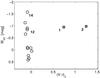 |
Fig. 1 Hertzsprung-Russell diagram of all analysed stars. MV0 is a mean V absolute magnitude corrected for extinction AV = 0.25 mag (Paunzen et al. 2011) assuming the distance modulus m − M = 18.49 mag as given by Pietrzyński et al. (2013); (V − I)0 is the colour index corrected for the corresponding interstellar reddening by 0.1 mag. Open circles clustering towards the main sequence indicate mCP candidates, the square denoted by 1 is the mean position of star 1 (135.3 4273), which is a short-period Cepheid. star 2 (135.30 107) is a normal non-variable K giant. Stars 12 and 14 are mCP candidates suspected for their rotationally modulated light variations. |
We compared our list of mCP candidate stars (Paunzen et al. 2006) with the OGLE database for corresponding measurements on the basis of equatorial coordinates and V magnitudes. After a first query, we inspected the positions in our original images and those of OGLE by eye. In total, we found fourteen matches in both sources. The final list of stars is given in Table 1.
A further analysis revealed that the sample of mCP candidates is contaminated by two late-type stars. The first, 135.3 4273, was recognised as the short-period Cepheid OGLE-LMC-CEP-0327 pulsating in its first overtone with the period P = 0.8821659(13) d (Soszyński et al. 2008). The second, 135.3 30 107, is a normal, non-variable K-type giant. We adopted them as control stars and their photometric data were analysed together with other stars of the sample. The Hertzsprung-Russell diagram of all studied stars constructed from data given in Table 1 is shown in Fig. 1.
The data of the mCP candidates contain the JDhel date of measurement,
ti, the measured V and I
magnitudes mi, and the estimate of its internal uncertainty
δmi. We have found that the last quantity
represents the real uncertainty of the magnitude determination quite well and that is why
we used it to weight the individual measurements according to the
relation  .
.
2.2. mCP star candidates
The mean V magnitudes of mCP candidates (stars 3–14) span the interval from 17.16 to 19.16 mag. Assuming a distance module (m − M) for the LMC of 18.33 mag and an extinction of AV = 0.25 mag (Paunzen et al. 2011), we obtain the interval of absolute V magnitudes from −1.4 to +0.6 mag, respectively. It corresponds mainly to Si-type of mCP stars, spectroscopically verified by Paunzen et al. (2011).
The median of the amplitude of light variations of mCP stars in V is
about 0.032 mag (Mikulášek et al. 2007a,b). The
typical error of the determination of one I measurement of our
mCP candidate set is σIt ~ 0.038 mag and the typical number of
measurements is NIt ~ 440 (see Table 1). Consequently, the expected uncertainty of
δIt of the amplitude determination of periodic variations
can be estimated as  mag. The same quantities for
V measurements are σVt ~ 0.015 mag and
NVt ~ 45,
mag. The same quantities for
V measurements are σVt ~ 0.015 mag and
NVt ~ 45,  mag. We found this encouraging
for the project of detecting periodicities in OGLE-III photometry.
mag. We found this encouraging
for the project of detecting periodicities in OGLE-III photometry.
Before starting the analysis of V and I photometric data we investigated the expected relationship between infrared and visual variations of mCP stars in more detail.
2.3. I light variability of mCP stars
Our search for periodic rotationally modulated variations in the sample of 12 LMC mCP candidates is based mainly on the analysis of the variability of these stars in the near infrared, while the Galactic mCP star variability is studied mainly in the visual region. Unfortunately, the information about the infrared variability of Galactic mCP stars is very scarce. From the few observations available (e.g. Musielok et al. 1980; Catalano et al. 1998; Wraight et al. 2012) one can conclude, that the amplitude of the light variations in the near infrared filters is similar but not identical to that in visual filters. This can be easily understood from the theoretical model of the light variability of mCP stars (Molnar 1975; Krtička et al. 2007; Shulyak et al. 2010), which is based on the light redistribution from the shorter wavelength region (typically the far ultraviolet) to the longer wavelength region (typically the visual and infrared) because of enhanced opacity in the regions with overabundant elements. The infrared continuum lies in the Rayleigh-Jeans part of the flux distribution function, where the ratio of the two different fluxes is independent of wavelength.
To derive a quantitative prediction for the mCP star light variability in the near infrared, we employed successful models of the visual light variability of HD 37776 (Krtička et al. 2007, Teff = 22 000 K), HR 7224 (Krtička et al. 2009, Teff = 14 500 K), and CU Vir (Krtička et al. 2012, Teff = 13 000 K) and predicted the light curves in the I filter. The light curves are calculated from the surface abundance maps of these stars (Kuschnig et al. 1999; Khokhlova et al. 2000; Lehmann et al. 2007) using TLUSTY model atmospheres and SYNSPEC spectrum synthesis code (Lanz & Hubeny 2003, 2007). For these stars, no observations in I are available.
The light curves are predicted using specific intensities filtered by appropriate
transmission curve. We fitted the OGLE transmission curve by a suitable formula with a
precision better than 3% in the form of
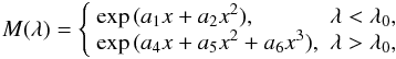 (1)where
the variable x is connected with the wavelength λ in Å
as
(1)where
the variable x is connected with the wavelength λ in Å
as 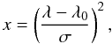 (2)and
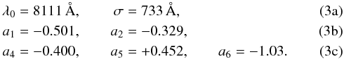 The
resulting light curves are given in Fig. 2. From this
plot we conclude that if the LMC mCP stars have the same amplitude as their Galactic
counterparts, their light variations should be detectable by OGLE.
The
resulting light curves are given in Fig. 2. From this
plot we conclude that if the LMC mCP stars have the same amplitude as their Galactic
counterparts, their light variations should be detectable by OGLE.
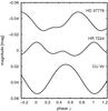 |
Fig. 2 Predicted light curves in the I band of selected Galactic mCP stars. |
3. Search for photometric periodicity
The detection of photometric variations of LMC mCP candidates is not straightforward because of their faintness. That is why we approximated their light behaviour by the simplest possible model assuming that light curves in all filters are simple sinusoidal with the same amplitude. Whenever a signal of this kind is detected, we are able to improve the model even more.
3.1. Periodograms
The periods of variable stars are usually inferred by means of various kinds of
periodograms. We opted for two versions of periodograms based on the fitting of detrended
measurements yi with
uncertainties σi done in the moments
ti by an ordinary sine-cosine model,
f(ω,t) = b1 cos(ω t) + b2 sin(ω t),
where ω = 2π/P is an
angular frequency and P the period, using the standard
χ2 least-squares method. If the sum
χ2(ω) is for the given ω
minimum the so-called modified amplitude
Am(ω) has to be maximum,
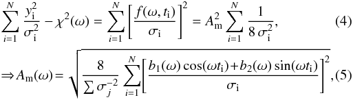 where
b1(ω) and
b2(ω) are coefficients of the fit. When
there is a uniform phase coverage, the modified amplitude is equal to the amplitude of
sinusoidal signal. The best phase sorting of the observed light variations corresponds to
the angular frequency ωm with the maximum of modified
amplitude Am(ω).
where
b1(ω) and
b2(ω) are coefficients of the fit. When
there is a uniform phase coverage, the modified amplitude is equal to the amplitude of
sinusoidal signal. The best phase sorting of the observed light variations corresponds to
the angular frequency ωm with the maximum of modified
amplitude Am(ω).
The second LSM type of periodogram uses for the significance of individual peaks a robust
signal-to-noise ratio (S/N) criterion, which is defined as 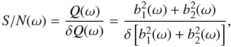 (6)where
δQ(ω) is an estimate of the uncertainty of the
quantity Q(ω) for a particular angular frequency.
(6)where
δQ(ω) is an estimate of the uncertainty of the
quantity Q(ω) for a particular angular frequency.
We tested the properties of the S/N(ω) criterion a thousand samples with sine signals scattered by randomly distributed noise. We found that if there is no periodic signal in this data, the median of the maximum S/N(ω) value in a periodogram is 4.52; in 95% of cases we find a S/N value between 4.2 and 5.4. The occurrence of peaks definitely higher than 6 indicates possible periodic variations. The detailed description of both LSM novel periodogram criteria will be published elsewhere.
During the treatment of OGLE-III time series, we concluded that both types of periodograms correlate very well with other time-proven estimates, the Lomb-Scargle (see e.g. Press & Rybicki 1989) periodogram, for example. So we are able to consider them as generally interchangeable.
We tested all frequencies from 0 to 2.1 d-1. The upper limit is slightly above
the frequency of the fastest rotating CP star known to date (HD 164429, with the period of
 , see Adelman 1999).
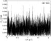 |
Fig. 3 Typical periodogram of a mCP candidate, star 4 (136.7.16501); all peaks are inconspicuous. |
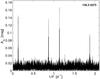 |
Fig. 4 Basic period of the overtone-Cepheid OGLE-LMC-CEP-0327 (135.3 4273) plus its aliases conjugated with the period of a sidereal day. |
3.2. Discussion of periodograms
We constructed periodograms for all stars of our sample and calculated frequencies f = 1/P of their maximum peaks and modified amplitudes Am and S/Ns for these peaks. These quantities are given in Table 1. We compared the periodograms of the LMC mCP candidates with those of the control stars, where we clearly detected the variability of OGLE-LMC-CEP-0327 and its aliases conjugated with the period of a sidereal day (Fig. 4). Our results exactly agree with the previous determination of the period and other characteristics of the star. This lends confidence to our time series analysis method.
The periodograms of the known Cepheid and the mCP candidates plus the second control star apparently differ: the peaks here have only a very narrow margin to the body of a pure scatter (compare Figs. 3 and 4). There are additional arguments to explain why all periods except those found for the stars 12 and probably star 14, listed in Table 1, are very likely only coincidences:
-
The distribution of the maximum amplitude frequencies isshallow and the found frequencies cover the studiedinterval 0 to 2.1 d-1 more or less evenly. This is a sign that observed peaks are most likely mere coincidences.
-
The median of periods of maximum amplitude, 1.0 d, differs significantly from the median period of Galactic mCP stars, 3.2 d (Mikulášek et al. 2007a,b).
-
The amplitudes of light changes of Galactic mCP stars display no correlation with colour index, spectral type, or absolute magnitude. It is in sharp contrast with observations of LMC mCP candidates whose observed maximum amplitudes exhibit strict monotonic dependence on the mean magnitude (see circles in Fig. 5). It suggests that the nature of observed variability of LMC objects is different.
-
It is conspicuous that the median of S/N of the highest peaks in periodograms of individual CP candidates is only 4.7, corresponding to the median of maxima peaks S/N = 4.52 in the case of pure scatter. It indicates the lack of detectable periodic signal in the majority of inspected mCP candidates, with two exceptions (stars 12 and 14) which are discussed in the following.
This persuaded us to test the hypothesis that the distribution of the data is random via a heuristic shuffling method. We re-analysed the data of each mCP candidate in the same way as described above, only we randomly shuffled all the individual observations (magnitudes and their uncertainties), the times of the observations remained the same. We are convinced that any periodic signal had to be destroyed. We calculated Ams and S/Ns for each shuffled version of data. The median of the both shuffled quantities is given in Table 1 and Fig. 5. It is apparent that the results are nearly the same as in the case of the original, unshuffled data with two exceptions (stars 12 and No 14).
As an added and independent test, we applied two different time series analysis methods, namely the modified Lafler-Kinman method (Hensberge et al. 1977) and the Phase-Dispersion-Method (Stellingwerf 1978). All computations were done within the programme package Peranso1. Using these utilities we find only upper limits for variability, but no statistically significant detection except for the case of star 1. The frequencies discussed in the following for stars 12 and 14, are detected on a 3.4 and 3.9σ level, respectively.
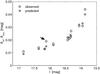 |
Fig. 5 Dependence of the maximum modified amplitudes of the observed (Am – circles) and the shuffled data (Ams – squares) on the mean I magnitude of mCP candidates. The largest positive relative deviation is found for the star 12 (190.1 1581) and is denoted by an arrow. |
3.3. Significance of the found periods
The characteristics of periodograms is strongly affected by the scatter of data; this forced us to treat the time series very carefully and to develop special techniques that enabled us to extract hidden information as effectively as possible.
3.3.1. Aliasing
The OGLE-III data used for our 12 LMC mCP candidates cover the whole observed time interval rather unevenly and caused a lot of prominent aliases which make the spectrum of periods relatively complex. Besides the dominant peak at the real frequency of variations, one may expect its aliases to be conjugated with the frequency of the Earth’s rotation and revolution around the Sun. However, the schedule of OGLE exposures was more complicated.
Time series of the stars in our sample representing both 660 V and 5816 I measurements were obtained from 2001 to 2008. The complete photometry was done only when the LMC was sufficiently high above the horizon. Consequently, 85% of the measurements were obtained in the time between 2.5 h before and after the passage of the LMC through the local meridian. Similarly, 85% of the observations were done during six months in a year starting from mid-September until mid-March. There is only a weak correlation between the number of measurements and the corresponding lunar phase. All of this influenced the appearance of the details of the periodograms of the light variations of the individual stars.
Because the determination of the position and significance is demanding, we used the method of the direct modelling of aliases spectra by simulating the result of observations of the object with a given frequency of a sine signal. The simulated periodogram of this situation then demonstrates the aliases spectrum and the mutual proportion of their individual peaks. An example of a simulated spectrum of this kind for the basic frequency of f = 1/P = 0.8075 d-1 is displayed in Fig. 6. By default, the principal aliases are, double peaks, while the basic peak is a triplet with a dominant central peak. This structure helped us to distinguish among real and alias peaks in the frequency spectrum.
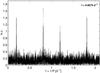 |
Fig. 6 Simulated periodogram for star 12 (190.1 1581) assuming a pure sine signal of the frequency f = 1/P = 0.8075 d-1. The most prominent peak corresponds to the basic frequency; the other pronounced peaks are conjugated aliases with one sidereal day. |
We conclude that each star has its specific aliases spectrum with different proportions in the heights of individual peaks and their inner structure.
3.3.2. Bootstrap tests
The bootstrap technique (Hall 1992) has proved to be very useful for testing the statistical significance and, therefore, the reality of found periods. It helped us to quantify this reality as a probability that the periodogram of a randomly created bootstrap subset of the original data has its dominant peak at the same frequency as the standard periodogram. We tested it with one hundred bootstrap subsets for each star of our sample. We consider a period to be statistically significant if the maximum peak occurs at one of the aliased frequencies because during the bootstrap choice aliases often exceed the basic peak. The probability of the period reality for each star is given in the column “prob” in Table 1.
The results are rather dismal. With the exception of the undoubtedly variable star 1, the reality of finding a star period never exceeds 50%. Nevertheless, two stars, 190.1 1581 and 190.1 15527, at least approach that limit.
4. The mCP candidates suspected of periodic light variations
Both objects suspected of periodic light variations, star 12 (190.1 1581) and star 14
(190.1 15527), display relatively low amplitude light variation which are only slightly
above the detectability by OGLE-III V and I photometry.
Therefore, we used a very simple model of their behaviour assuming the linear ephemeris and
the sine form of the V and I variations with different
amplitudes. We obtained the following model of light changes 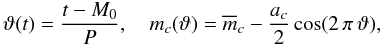 (7)where
ϑ(t) is a phase function, M0
is the moment of the basic maximum, P is the period in days,
mc(t) is a predicted
magnitude in filter
c (c = V, I) at the
time t,
(7)where
ϑ(t) is a phase function, M0
is the moment of the basic maximum, P is the period in days,
mc(t) is a predicted
magnitude in filter
c (c = V, I) at the
time t,  is a mean value of
the magnitude in the filter c, and
ac is an amplitude in the filter
c. The values for both stars derived by standard least-squares
minimization regression are given in Table 2.
is a mean value of
the magnitude in the filter c, and
ac is an amplitude in the filter
c. The values for both stars derived by standard least-squares
minimization regression are given in Table 2.
4.1. LMC 190.1 1581
Star 12 (190.1 1581) is one of the brighter stars in our sample. Its mean absolute
magnitude  mag and negative
dereddened index
mag and negative
dereddened index  mag
indicates that this object belongs among the late B-type stars. If it is a true mCP star,
it is most likely a Si- or He-weak type object.
mag
indicates that this object belongs among the late B-type stars. If it is a true mCP star,
it is most likely a Si- or He-weak type object.
In its periodogram we find a dominant peak at the frequency
f = 0.8075 d-1 corresponding to the period
 . The second peak of
nearly the same height consists of two peaks at the frequencies
f = 1.8075 d-1 and
f = 1.81025 d-1. Their distance of 0.00275 d-1
corresponds to the reciprocal value of the sidereal year in days. The internal structure
indicates that it is an alias of the basic period. The bootstrap test of the reality of
the found period gives 49%, which is the absolute maximum among the mCP candidates in our
sample.
. The second peak of
nearly the same height consists of two peaks at the frequencies
f = 1.8075 d-1 and
f = 1.81025 d-1. Their distance of 0.00275 d-1
corresponds to the reciprocal value of the sidereal year in days. The internal structure
indicates that it is an alias of the basic period. The bootstrap test of the reality of
the found period gives 49%, which is the absolute maximum among the mCP candidates in our
sample.
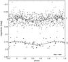 |
Fig. 7 V and I light curves of star 12 (190.1 1581) plotted according to the ephemeris given in Table 2. |
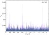 |
Fig. 8 Comparison of the classical Lomb-Scargle periodogram of star 12 (190.1 1581) before (pale magenta) and after subtraction (dark blue) of the variations described by the model (Eq. (7)). It seems that a substantial part of the variability of the star is well described by this model and its parameters (Table 2). |
A careful inspection of CCD images of this star reveals that it is a visual binary with a companion that is about 1.5 mag fainter than our target. The OGLE-III photometry was apparently done for both components. Future photometric observations and treatments of them should take this into account. On the other hand, the modest ratio of amplitudes of variations in V and I filters completely fulfills our theoretical expectation.
4.2. LMC 190.1 15 527
Star 14 (190.1 15 527) is the brightest and one of the hottest mCP candidates in our
sample. With MV0 = −1.57 mag and
(V − I)0 = −0.09 mag it is a late
Bp star with Si or He-weak chemical peculiarity. The most striking result of its analysis
is the found period of  , which is rather short. If it
is confirmed, it would be one of the fastest rotating mCP stars detected so far.
, which is rather short. If it
is confirmed, it would be one of the fastest rotating mCP stars detected so far.
Unfortunately, the found period shorter than 12 h is not as firmly established as in the case of the previous mCP candidate with larger light changes. It results in the relatively low appreciation of the reality probability of the found period only 30%. The rather small variations in the I filter (see Fig. 9) are also not in favour of variability, nor are our simulations with randomly distributed magnitudes that also constitute periodogram peaks slightly larger than 2 and 1. That is why we suspect the feature to be an artefact caused by the specifically distributed observations. However, Fig. 10 shows the success of the expression of the light curves by the simple model given in Eq. (7).
In conclusion, we suggest that the periodic variations of star 14 (190.1 15527) remains an open question.
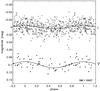 |
Fig. 9 V and I light curves of star 14 (190.1 15527) plotted according to the ephemeris given in Table 2. |
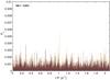 |
Fig. 10 Comparison of the classical Lomb-Scargle periodogram of the star No. 14 – 190.1 15527 before (pale colour) and after (dark colour) subtraction of the variations described by the model (Eq. (7)). It seems that a part of the variability of the star can be described by this model and found parameters (see Table 2). Unfortunately, there are some indications that the main peak may be an artefact caused by specifically distributed data. |
5. Conclusions
We analysed the OGLE-III photometry for fourteen stars of which twelve are mCP candidates. In total, 6476 individual photometric measurements in V and I were used to perform a time series analysis. For this purpose, we calculated periodograms including a bootstrap-based probability of the statistical significance. Although the median of the amplitudes of maximum peaks, median Am = 0.02 mag in the periodograms of the mCP candidates, does not contradict our expectation (median(Am) = 0.032 mag for Galactic mCP stars; Mikulášek et al. 2007a,b), other circumstances suggest that the prevailing majority of these peaks might not be statistically significant. We found some periodic variations in only two of the mCP candidates, of which one is doubtful.
It seems that the rotationally modulated variability of the studied mCP candidates in the V and I bands is very weak (if present at all). As upper limits of their effective amplitudes, we used Aeffs derived from the analysis of shuffled data. Nevertheless, it is very likely that the true amplitudes are much lower than 0.01 mag, which is the limit derived from the time series analysis of the brightest mCP candidate.
From this finding we can conclude that the spots on the stellar surfaces of these objects are not as contrasting as those of their Galactic counterparts; in other words, the overabundant elements (Si, Fe, Cr, and so on) are more evenly distributed over the surface or the maximum abundance is lower. This phenomenon has also been observed for non-magnetic Galactic Am or weakly magnetic HgMn stars.
The low contrast of LMC mCP photometric spots could be explained by lower global magnetic fields strengths of LMC mCP stars than their Galactic counterparts. It may relate with the lower level of interstellar magnetic field in the LMC if we compare it with the Galactic field, which results in the overall lower percentage of mCP star appearance compared to the Milky Way (Paunzen et al. 2006).
Our results could also have a fundamental impact on the origin of the global stellar magnetic fields for those objects. Two theories have been developed for this (Moss 1989), and are still in dispute. The fossil theory has two variants: the magnetic field is either the slowly decaying relic of the frozen-in interstellar magnetic field or of the dynamo acting in the pre-main sequence phase. The dynamo theory is based on the existence of a contemporaneous dynamo operating in the convective core of the magnetic stars. If we assume that the stellar dynamo functions with the same efficiency for all stars with an identical mass and luminosity, than we should find the same number of mCP stars in the Milky Way and the LMC. On the other hand, the global magnetic field of the LMC (≈ 1.1 μG, Gaensler et al. 2005) is much weaker than that of the Milky Way (6–10 μG, Beck 2009). Therefore, our results are in favour of the fossil theory being the cause of the CP star phenomenon.
Another important global parameter which has to be taken into account is the metallicity. The overall metallicity of the LMC is about −0.5 to −2.0 dex lower than that of the Milky Way. For the CP phenomenon, in general, besides Fe, Mg, Si, and Cr are the most important elements for the light variability
and thus the spot characteristics. Our targets are members of or in the surrounding of the open clusters NGC 1711, NGC 1866, and NGC 2136/7. In addition, one field in the bulge was observed. The published [Fe/H] values for those regions are all below −0.70 dex (Paunzen et al. 2006). Pompéia et al. (2008) published detailed [α/Fe] ratios for the inner disc of LMC. They conclude that the abundances of Mg, Si, Ti, and Cr scale the same way as [Fe/H]. The intrinsic abundance of our targets should be, therefore, uniform, not favouring any element for magnetic diffusion and thus the spot characteristics or the maximum elemental abundances are too low to cause any substantial light variability.
As future steps, we suggest retrieving time series of the remaining published mCP candidate stars and getting more accurate measurements of the presented stars. In addition, observations in other wavelength regions would shed more light on the surface characteristics.
Online material
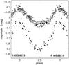 |
Fig. 11 V (◆) and I (°) light curves of star 1 (135.3 4273) plotted according to the ephemeris given in Table 2. |
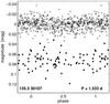 |
Fig. 12 V (◆) and I (°) light curves of star 2 (135.3 30107) plotted according to the ephemeris given in Table 2. |
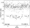 |
Fig. 13 V (◆) and I (°) light curves of star 3 (136.7 861) plotted according to the ephemeris given in Table 2. |
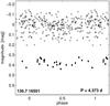 |
Fig. 14 V (◆) and I (°) light curves of star 4 (136.7 16501) plotted according to the ephemeris given in Table 2. |
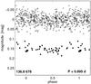 |
Fig. 15 V (◆) and I (°) light curves of star 5 (136.8 678) plotted according to the ephemeris given in Table 2. |
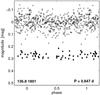 |
Fig. 16 V (◆) and I (°) light curves of star 6 (136.8 1801) plotted according to the ephemeris given in Table 2. |
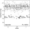 |
Fig. 17 V (◆) and I (°) light curves of star 7 (136.8 1873) plotted according to the ephemeris given in Table 2. |
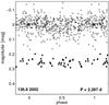 |
Fig. 18 V (◆) and I (°) light curves of star 8 (136.8 2002) plotted according to the ephemeris given in Table 2. |
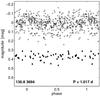 |
Fig. 19 V (◆) and I (°) light curves of star 9 (136.8 3694) plotted according to the ephemeris given in Table 2. |
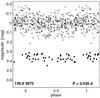 |
Fig. 20 V (◆) and I (°) light curves of star 10 (136.8 3875) plotted according to the ephemeris given in Table 2. |
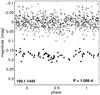 |
Fig. 21 V (◆) and I (°) light curves of star 11 (190.1 1445) plotted according to the ephemeris given in Table 2. |
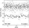 |
Fig. 22 V (◆) and I (°) light curves of star 13 (190.1 2822) plotted according to the ephemeris given in Table 2. |
Acknowledgments
This work was supported by the following grants: GA ČR P209/12/0217, 7AMB12AT003, WTZ CZ-10/2012, #LG12001 (Czech Ministry of Education, Youth and Sports), and FWF P22691-N16. The OGLE project has received funding from the European Research Council under the European Community’s Seventh Framework Programme (FP7/2007-2013)/ERC grant agreement No. 246678. We dedicate this paper to Willy Schreiner who tragically died during its writing.
References
- Adelman, S. 1999, A&AS, 136, 379 [NASA ADS] [CrossRef] [EDP Sciences] [Google Scholar]
- Beck, R. 2009, Proc. IAU Symp., 259, 3 [NASA ADS] [Google Scholar]
- Catalano, F. A., Leone, F., & Kroll, R. 1998, A&AS, 131, 63 [NASA ADS] [CrossRef] [EDP Sciences] [Google Scholar]
- Gaensler, B. M., Haverkorn, M., Staveley-Smith, L., et al. 2005, Science, 307, 1610 [NASA ADS] [CrossRef] [PubMed] [Google Scholar]
- Hall, P. 1992, The Bootstrap and Edgeworth Expansion (New York: Springer) [Google Scholar]
- Hensberge, H., de Loore, C., Zuiderwijk, E. J., & Hammerschlag-Hensberge, G. 1977, A&A, 54, 443 [NASA ADS] [Google Scholar]
- Khokhlova, V. L., Vasilchenko, D. V., Stepanov, V. V., & Romanyuk, I. I. 2000, Astron. Lett., 26, 177 [Google Scholar]
- Krtička, J., Mikulášek, Z., Zverko, J., & Žižňovský, J. 2007, A&A, 470, 1089 [NASA ADS] [CrossRef] [EDP Sciences] [Google Scholar]
- Krtička, J., Mikulášek, Z., Henry, G. W., et al. 2009, A&A, 499, 567 [NASA ADS] [CrossRef] [EDP Sciences] [Google Scholar]
- Krtička, J., Mikulášek, Z., Lüftinger, T., et al. 2012, A&A, 537, A14 [NASA ADS] [CrossRef] [EDP Sciences] [Google Scholar]
- Kuschnig, R., Ryabchikova, T. A., Piskunov, N. E., Weiss, W. W., & Gelbmann, M. J. 1999, A&A, 348, 924 [NASA ADS] [Google Scholar]
- Lanz, T., & Hubeny, I. 2003, ApJS, 146, 417 [NASA ADS] [CrossRef] [Google Scholar]
- Lanz, T., & Hubeny, I. 2007, ApJS, 169, 83 [CrossRef] [Google Scholar]
- Lehmann, H., Tkachenko, A., Fraga, L., Tsymbal, V., & Mkrtichian, D. E. 2007, A&A, 471, 941 [NASA ADS] [CrossRef] [EDP Sciences] [Google Scholar]
- Maitzen, H. M., Paunzen, E., & Pintado, O. I. 2001, A&A, 371, L5 [NASA ADS] [CrossRef] [EDP Sciences] [Google Scholar]
- Mikulášek, Z., Janík, J., Zverko, J., et al. 2007a, Astron. Nachr., 328, 10 [NASA ADS] [CrossRef] [Google Scholar]
- Mikulášek, Z., Zverko, J., Krtička, J., et al. 2007b, in Magnetic Stars, eds. I. Romanyuk, & D. Kudryavtsev, 352 [Google Scholar]
- Molnar, M. R. 1975, AJ, 80, 173 [NASA ADS] [CrossRef] [Google Scholar]
- Moss, D. 1989, MNRAS, 236, 629 [NASA ADS] [Google Scholar]
- Musielok, B., Lange, D., Schoenich, W., et al. 1980, Astron. Nacher., 301, 71 [Google Scholar]
- Patterson, R. S., & Neff, J. S. 1979, ApJS, 41, 215 [NASA ADS] [CrossRef] [Google Scholar]
- Paunzen, E., Stütz, Ch., & Maitzen, H. M. 2005, A&A, 441, 631 [NASA ADS] [CrossRef] [EDP Sciences] [Google Scholar]
- Paunzen, E., Maitzen, H. M., Pintado, O. I., et al. 2006, A&A, 459, 871 [NASA ADS] [CrossRef] [EDP Sciences] [Google Scholar]
- Paunzen, E., Netopil, M., & Bord, D. J. 2011, MNRAS, 411, 260 [NASA ADS] [CrossRef] [Google Scholar]
- Pietrzyński, G., Graczyk, D., Gieren, W., et al. 2013, Nature, 495, 76 [NASA ADS] [CrossRef] [PubMed] [Google Scholar]
- Pompéia, L., Hill, V., Spite, M., et al. 2008, A&A, 480, 379 [NASA ADS] [CrossRef] [EDP Sciences] [Google Scholar]
- Press, W. H., & Rybicki, G. B. 1989, ApJ, 338, 277 [NASA ADS] [CrossRef] [Google Scholar]
- Renson, P., & Catalano, F. A. 2001, A&A, 378, 113 [NASA ADS] [CrossRef] [EDP Sciences] [Google Scholar]
- Soszyński, I., Poleski, R., Udalski, A., et al. 2008, Acta Astron., 58, 163 [NASA ADS] [Google Scholar]
- Shulyak, D., Krtička, J., Mikulášek, Z., et al. 2010, A&A, 524, A6 [NASA ADS] [CrossRef] [EDP Sciences] [Google Scholar]
- Stellingwerf, R. F. 1978, ApJ, 224, 953 [NASA ADS] [CrossRef] [Google Scholar]
- Stibbs, D. W. N. 1950, MNRAS, 110, 395 [NASA ADS] [CrossRef] [Google Scholar]
- Udalski, A., Szymański, M. K., Soszyński, I., & Poleski, R. 2008, Acta Astron., 58, 69 [NASA ADS] [Google Scholar]
- Wraight, K. T., Fossati, L., Netopil, M., et al. 2012, MNRAS, 420, 757 [NASA ADS] [CrossRef] [Google Scholar]
All Tables
Basic photometric parameters from Paunzen et al. (2006) and references therein, as well as the photometric characteristics of CP candidates in the V and I bands.
All Figures
|
Fig. 1 Hertzsprung-Russell diagram of all analysed stars. MV0 is a mean V absolute magnitude corrected for extinction AV = 0.25 mag (Paunzen et al. 2011) assuming the distance modulus m − M = 18.49 mag as given by Pietrzyński et al. (2013); (V − I)0 is the colour index corrected for the corresponding interstellar reddening by 0.1 mag. Open circles clustering towards the main sequence indicate mCP candidates, the square denoted by 1 is the mean position of star 1 (135.3 4273), which is a short-period Cepheid. star 2 (135.30 107) is a normal non-variable K giant. Stars 12 and 14 are mCP candidates suspected for their rotationally modulated light variations. |
| In the text | |
|
Fig. 2 Predicted light curves in the I band of selected Galactic mCP stars. |
| In the text | |
|
Fig. 3 Typical periodogram of a mCP candidate, star 4 (136.7.16501); all peaks are inconspicuous. |
| In the text | |
|
Fig. 4 Basic period of the overtone-Cepheid OGLE-LMC-CEP-0327 (135.3 4273) plus its aliases conjugated with the period of a sidereal day. |
| In the text | |
|
Fig. 5 Dependence of the maximum modified amplitudes of the observed (Am – circles) and the shuffled data (Ams – squares) on the mean I magnitude of mCP candidates. The largest positive relative deviation is found for the star 12 (190.1 1581) and is denoted by an arrow. |
| In the text | |
|
Fig. 6 Simulated periodogram for star 12 (190.1 1581) assuming a pure sine signal of the frequency f = 1/P = 0.8075 d-1. The most prominent peak corresponds to the basic frequency; the other pronounced peaks are conjugated aliases with one sidereal day. |
| In the text | |
|
Fig. 7 V and I light curves of star 12 (190.1 1581) plotted according to the ephemeris given in Table 2. |
| In the text | |
|
Fig. 8 Comparison of the classical Lomb-Scargle periodogram of star 12 (190.1 1581) before (pale magenta) and after subtraction (dark blue) of the variations described by the model (Eq. (7)). It seems that a substantial part of the variability of the star is well described by this model and its parameters (Table 2). |
| In the text | |
|
Fig. 9 V and I light curves of star 14 (190.1 15527) plotted according to the ephemeris given in Table 2. |
| In the text | |
|
Fig. 10 Comparison of the classical Lomb-Scargle periodogram of the star No. 14 – 190.1 15527 before (pale colour) and after (dark colour) subtraction of the variations described by the model (Eq. (7)). It seems that a part of the variability of the star can be described by this model and found parameters (see Table 2). Unfortunately, there are some indications that the main peak may be an artefact caused by specifically distributed data. |
| In the text | |
|
Fig. 11 V (◆) and I (°) light curves of star 1 (135.3 4273) plotted according to the ephemeris given in Table 2. |
| In the text | |
|
Fig. 12 V (◆) and I (°) light curves of star 2 (135.3 30107) plotted according to the ephemeris given in Table 2. |
| In the text | |
|
Fig. 13 V (◆) and I (°) light curves of star 3 (136.7 861) plotted according to the ephemeris given in Table 2. |
| In the text | |
|
Fig. 14 V (◆) and I (°) light curves of star 4 (136.7 16501) plotted according to the ephemeris given in Table 2. |
| In the text | |
|
Fig. 15 V (◆) and I (°) light curves of star 5 (136.8 678) plotted according to the ephemeris given in Table 2. |
| In the text | |
|
Fig. 16 V (◆) and I (°) light curves of star 6 (136.8 1801) plotted according to the ephemeris given in Table 2. |
| In the text | |
|
Fig. 17 V (◆) and I (°) light curves of star 7 (136.8 1873) plotted according to the ephemeris given in Table 2. |
| In the text | |
|
Fig. 18 V (◆) and I (°) light curves of star 8 (136.8 2002) plotted according to the ephemeris given in Table 2. |
| In the text | |
|
Fig. 19 V (◆) and I (°) light curves of star 9 (136.8 3694) plotted according to the ephemeris given in Table 2. |
| In the text | |
|
Fig. 20 V (◆) and I (°) light curves of star 10 (136.8 3875) plotted according to the ephemeris given in Table 2. |
| In the text | |
|
Fig. 21 V (◆) and I (°) light curves of star 11 (190.1 1445) plotted according to the ephemeris given in Table 2. |
| In the text | |
|
Fig. 22 V (◆) and I (°) light curves of star 13 (190.1 2822) plotted according to the ephemeris given in Table 2. |
| In the text | |
Current usage metrics show cumulative count of Article Views (full-text article views including HTML views, PDF and ePub downloads, according to the available data) and Abstracts Views on Vision4Press platform.
Data correspond to usage on the plateform after 2015. The current usage metrics is available 48-96 hours after online publication and is updated daily on week days.
Initial download of the metrics may take a while.