| Issue |
A&A
Volume 555, July 2013
|
|
|---|---|---|
| Article Number | A148 | |
| Number of page(s) | 12 | |
| Section | Numerical methods and codes | |
| DOI | https://doi.org/10.1051/0004-6361/201321725 | |
| Published online | 17 July 2013 | |
Stable higher order finite-difference schemes for stellar pulsation calculations
1
Institut d’Astrophysique et Géophysique de l’Université de
Liège,
Allée du 6 Août 17,
4000
Liège,
Belgium
e-mail: This email address is being protected from spambots. You need JavaScript enabled to view it.
2
Observatoire de Paris, LESIA, CNRS UMR 8109,
92195
Meudon,
France
Received:
17
April
2013
Accepted:
5
June
2013
Abstract
Context. Calculating stellar pulsations requires high enough accuracy to match the quality of the observations. Many current pulsation codes apply a second-order finite-difference scheme, combined with Richardson extrapolation to reach fourth-order accuracy on eigenfunctions. Although this is a simple and robust approach, a number of drawbacks exist that make fourth-order schemes desirable. A robust and simple finite-difference scheme that can easily be implemented in either 1D or 2D stellar pulsation codes, is therefore required.
Aims. One of the difficulties in setting up higher order finite-difference schemes for stellar pulsations is the so-called mesh-drift instability. Current ways of dealing with this defect include introducing artificial viscosity or applying a staggered grid approach; however, these remedies are not well-suited to eigenvalue problems, especially those involving non-dissipative systems, because they unduly change the spectrum of the operator, introduce supplementary free parameters, or lead to complications when applying boundary conditions.
Methods. We propose here a new method, inspired from the staggered grid strategy, which removes this instability while bypassing the above difficulties. Furthermore, this approach lends itself to superconvergence, a process in which the accuracy of the finite differences is boosted by one order.
Results. This new approach is successfully applied to stellar pulsation calculations, and is shown to be accurate, flexible with respect to the underlying grid, and able to remove mesh drift.
Conclusions. Although specifically designed for stellar pulsation calculations, this method can easily be applied to many other physical or mathematical problems.
Key words: methods: numerical / methods: analytical / stars: oscillations / stars: rotation
© ESO, 2013
1. Introduction
Numerically calculating pulsation modes in stellar models typically involves solving a differential system for which the coefficients change by several orders of magnitude and in which the underlying grid can be highly uneven. Currently, many stellar pulsation codes use a second-order finite-difference scheme combined with Richardson extrapolation to achieve high enough accuracy for the frequencies (Richardson & Gaunt 1927; Moya et al. 2008). Although this approach is robust and simple, it has some disadvantages. Firstly, the frequencies are accurate to fourth order, but the eigenfunctions only to the second. Secondly, Richardson extrapolation requires calculating the pulsation modes for two different resolutions, typically with N and N/2 points. These solutions then need to be matched correctly before applying the extrapolation. Although this is straightforward in most cases, it may be more challenging in red giant stars. Indeed, non-radial modes in such stars have a mixed p- and g-mode behaviour, thus resulting in a high density of nodes in the inner regions of the star (e.g. Dupret et al. 2009). Special care is needed to correctly match the modes, which furthermore need to be fully resolved at both resolutions. A third difficulty, which is illustrated in Sect. 5.1, is that the Richardson extrapolation is only strictly valid when the additional points from the denser grid lie at the midpoints of the coarser grid.
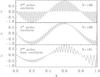 |
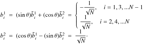
Fig. 1 Spurious numerical solutions to Eq. (1) caused by mesh drift, using a 2nd order finite-difference scheme on a uniform grid (upper panel), a 4th order scheme on a uniform grid (middle panel), and a 2nd order scheme on a non-uniform grid. The number of grid points, N, is indicated in the upper right corner of each panel. |
A way to circumvent these difficulties is to apply a fourth-order scheme or a higher one. This is the approach taken in the OSCROX (Roxburgh 2008), CAFein (Valsecchi et al. 2013), PULSE (Brassard & Charpinet 2008) and LOSC (Scuflaire et al. 2008) oscillations codes. When devising the stellar oscillation code TOP (Two-dimensional Oscillation Program Reese et al. 2006, 2009), a fourth or higher order approach was also searched for. Given that this code uses an algebraic rather than a shooting method for finding the eigensolutions, applying a fourth-order Runge-Kutta method, such as what is done in OSCROX and CAFein, is inappropriate. Gautschy & Glatzel (1990) and Takata & Löffler (2004), upon which the CAFein code is built, use predictor-corrector schemes to integrate the pulsation equations, which were reformulated through the Riccati method. Such schemes can be set up to fourth or higher order accuracy, but much like the Runge-Kutta integrator, they are also unsuitable for an algebraic method.
Besides the requirements imposed by its algebraic approach, TOP also needs a scheme which is simple and robust, since it is designed to handle pulsation modes in rapidly rotating stars, a 2D problem. The PULSE code uses a finite element approach (Brassard et al. 1992), which although accurate and stable, leads to a higher complexity in the program due to the need to integrate the products of equilibrium quantities and basis functions over each element. A finite-difference approach is simpler, since the discretised form of the differential equations only involve coefficients which are the products of equilibrium quantities and finite-difference coefficients. Accordingly, the approach implemented in the LOSC code is closest to these requirements since it is a fourth-order finite-difference scheme (Scuflaire et al. 2008). Nonetheless, the main drawback with this scheme is that it requires calculating radial derivatives of equilibrium quantities, which can be an additional source of error, especially in evolved models with steep compositional, hence density, gradients. Therefore, a simpler fourth or higher order finite-difference scheme was searched for when developing TOP.
A first, and somewhat naive, form of higher order finite differences was initially implemented in TOP (Reese et al. 2009). However, a numerical instability known as mesh drift appeared, thereby leading to oscillatory behaviour and spurious modes. Prior to this, Dupret (2001) also reports on similar difficulties when setting up the non-adiabatic pulsation code called MAD. The goal of the present paper is therefore to search for some of the causes behind mesh drift and to propose a remedy. In the following section, the problem of mesh drift is described, illustrated and characterised. Section 3 then proposes a new method for dealing with mesh drift and compares it with other approaches. The following section shows how this new approach can be enhanced through “superconvergence”, which boosts the order of the finite differences by one. Section 5 describes and evaluates 1D and 2D stellar pulsation calculations based on this new approach. Finally, the paper ends with a short conclusion.
2. Mesh drift
It has been known for many years that finite-difference schemes can suffer from mesh-drift instability. This instability typically involves the decoupling of even and odd grid points in the differences equations (e.g. Press et al. 2007). Depending on the differential problem which is being solved, this can lead to solutions with highly oscillatory behaviour or spurious solutions.
2.1. Examples of mesh-drift instability
In order to illustrate some of the difficulties caused by mesh drift, we propose to
numerically solve the following trivial eigenvalue problem over the interval
[0,1] :  (1)where
ω is the eigenvalue and primes denote first-order derivatives with
respect to the variable x. The solutions are
u(x) = Asin(ωx),
v(x) = Acos(ωx),
where ω = kπ, k is an integer, and
A an arbitrary non-zero constant.
(1)where
ω is the eigenvalue and primes denote first-order derivatives with
respect to the variable x. The solutions are
u(x) = Asin(ωx),
v(x) = Acos(ωx),
where ω = kπ, k is an integer, and
A an arbitrary non-zero constant.
In the first case, we use a uniform grid and a second-order scheme defined over a
three-point window. On the end points, we replace the above formula by a first-order
scheme defined on a two-point window so as to avoid introducing supplementary bands in the
matrix representation of the derivation operator which takes on a banded form. Avoiding
supplementary bands can be important for reducing the numerical cost of large scale
computations, where the number of bands in the total system depends critically on that of
the derivation operator. The boundary conditions are imposed by replacing two of the
2N difference equations. Hence, the resultant difference equations are:
 (2)where
N is the number of grid points, and
Δx = xi + 1 − xi.
Although the correct solutions are well recovered, supplementary spurious solutions appear
such as the one in the upper panel of Fig. 1, with an
eigenvalue around 2.5π.
(2)where
N is the number of grid points, and
Δx = xi + 1 − xi.
Although the correct solutions are well recovered, supplementary spurious solutions appear
such as the one in the upper panel of Fig. 1, with an
eigenvalue around 2.5π.
One may then try a fourth-order scheme using windows with five grid points (xi − 2,...xi + 2) with reduced order schemes near the endpoints and boundary conditions which replace two of the difference equations, as was done above. The middle panel of Fig. 1 illustrates a similar spurious solution.
Finally, the last panel shows the results for a second-order scheme using three-point
windows (except at the endpoints) and using a non-uniform grid:  (3)Furthermore, we changed
the number of grid points from N = 100 to N = 101. The
finite-difference weights involved were deduced from Fornberg (1988). Once more, similar spurious solutions appear, such as the one
illustrated in the lower panel of Fig. 1. These last
two examples show that mesh drift is, in fact, a more general problem than simply a
decoupling between even and odd grid points, given that all the points are coupled in
these latter two schemes. Also, the last example shows that the problem occurs regardless
of whether N is even or odd. This raises the questions as to when mesh
drift occurs and how to remove it.
(3)Furthermore, we changed
the number of grid points from N = 100 to N = 101. The
finite-difference weights involved were deduced from Fornberg (1988). Once more, similar spurious solutions appear, such as the one
illustrated in the lower panel of Fig. 1. These last
two examples show that mesh drift is, in fact, a more general problem than simply a
decoupling between even and odd grid points, given that all the points are coupled in
these latter two schemes. Also, the last example shows that the problem occurs regardless
of whether N is even or odd. This raises the questions as to when mesh
drift occurs and how to remove it.
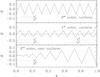 |
Fig. 2 Null space basis functions for the finite-difference schemes used in Fig. 1 (except that the resolution has been reduced for the sake of legibility). The functions (b1,b2...bD) are ordered such that the most oscillatory function comes first. |
2.2. Characterising mesh drift
In the first example above, mesh drift occurred because even and odd points were decoupled. Another way of looking at this is that the numerical derivative of a function, f, defined such that f(x) = a for even points and f(x) = b for odd points, where a and b are two distinct constants, will be zero (except at the end points where a different scheme is used). Hence, one may generalise this and look for functions which numerically satisfy the relation f′ = 0 for other schemes.
In order to avoid only having a constant solution, we impose
f′ = 0 only over the interval which allows full windows for
the different schemes above. Hence, for a three-point second-order scheme, we will impose:
 (4)where
 denotes
finite-difference weights at point i (in the case of a uniform grid,
will only
depend on j). For a five-point fourth-order scheme, we have:
denotes
finite-difference weights at point i (in the case of a uniform grid,
will only
depend on j). For a five-point fourth-order scheme, we have:
 (5)For the
second-order schemes, the resultant null space will be of dimension D = 2
since there are N − 2 equations for N unknowns.
Likewise, the null space for fourth-order schemes will be of dimension
D = 4. In both cases, the null space will include constant functions,
which are the correct solutions to the problem.
(5)For the
second-order schemes, the resultant null space will be of dimension D = 2
since there are N − 2 equations for N unknowns.
Likewise, the null space for fourth-order schemes will be of dimension
D = 4. In both cases, the null space will include constant functions,
which are the correct solutions to the problem.
An orthogonal basis1,
 , for the null space of the
above system can be extracted by calculating, for example, a singular value decomposition
of its representative matrix (made up of the coefficients
). However, to
go one step further, it is helpful to find a new basis which brings out the most
oscillatory solutions. We therefore introduce the following quadratic form which measures
how oscillatory a given function,
(gi)i = 1...N,
is:
, for the null space of the
above system can be extracted by calculating, for example, a singular value decomposition
of its representative matrix (made up of the coefficients
). However, to
go one step further, it is helpful to find a new basis which brings out the most
oscillatory solutions. We therefore introduce the following quadratic form which measures
how oscillatory a given function,
(gi)i = 1...N,
is: 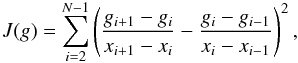 (6)and search for
normalised elements which maximise this measure. It is straightforward to see that
J = 0 only for elements with a constant slope (i.e.
gi = axi + b,
where a and b are constants). To make sure we find
solutions within the null space, we decompose g over the
(6)and search for
normalised elements which maximise this measure. It is straightforward to see that
J = 0 only for elements with a constant slope (i.e.
gi = axi + b,
where a and b are constants). To make sure we find
solutions within the null space, we decompose g over the
 basis, i.e.
  ,
and re-express the quadratic form in terms of the coordinates
(μj)j = 1...D:
,
and re-express the quadratic form in terms of the coordinates
(μj)j = 1...D:
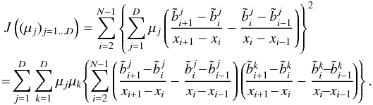 (7)By
virtue of the Rayleigh-Ritz theorem, the normalised vectors which maximise and minimise
J are the eigenvectors associated with the maximal and minimal
eigenvalues of J. Moreover, the set of eigenvectors of J
can be expressed as a new orthogonal basis,
ℬ = (b1,b2...bD),
of the null space2.
(7)By
virtue of the Rayleigh-Ritz theorem, the normalised vectors which maximise and minimise
J are the eigenvectors associated with the maximal and minimal
eigenvalues of J. Moreover, the set of eigenvectors of J
can be expressed as a new orthogonal basis,
ℬ = (b1,b2...bD),
of the null space2.
In order to illustrate how the above procedure works, we apply it to the second-order
scheme defined over a uniform grid. This leads to the following set of equations:
 (8)A singular value
decomposition of the representative matrix yields an orthogonal basis of the null space,
for example:
(8)A singular value
decomposition of the representative matrix yields an orthogonal basis of the null space,
for example: 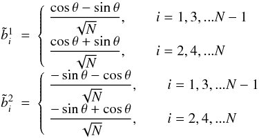 (9)where
θ is an arbitrary number and where we have assumed, for simplicity,
that N is even. One can easily verify that the above functions satisfy
Eq. (8) and form an orthogonal basis.
However, unless θ is a multiple of
π/2, both basis functions contain both an oscillatory
and a constant component. Nonetheless, what we want is a basis in which one of the two
solutions is the most oscillatory, and the other, the least oscillatory, i.e. constant.
This is where the second step of the procedure intervenes. Using Eq. (7), we begin by expressing the quadratic form
J in terms of the reduced coordinates
(μ1,μ2):
(9)where
θ is an arbitrary number and where we have assumed, for simplicity,
that N is even. One can easily verify that the above functions satisfy
Eq. (8) and form an orthogonal basis.
However, unless θ is a multiple of
π/2, both basis functions contain both an oscillatory
and a constant component. Nonetheless, what we want is a basis in which one of the two
solutions is the most oscillatory, and the other, the least oscillatory, i.e. constant.
This is where the second step of the procedure intervenes. Using Eq. (7), we begin by expressing the quadratic form
J in terms of the reduced coordinates
(μ1,μ2):
![Mathematical equation: \begin{equation} J(\mu_1,\mu_2) = \left[ \begin{array}{cc} \mu_1 & \mu_2 \end{array} \right] \left[\begin{array}{cc} \Lambda \sin^2 \theta & \Lambda \sin\theta \cos\theta \\ \Lambda \sin\theta \cos\theta & \Lambda \cos^2 \theta \end{array} \right] \left[ \begin{array}{c} \mu_1 \\ \mu_2 \end{array} \right], \end{equation}](/articles/aa/full_html/2013/07/aa21725-13/aa21725-13-eq51.png) (10)where
(10)where
 .
The eigenvectors of J are (sinθ,cosθ),
associated with the eigenvalue Λ, and (cosθ, − sinθ),
associated with the eigenvalue 0. This leads to the following orthogonal basis:
.
The eigenvectors of J are (sinθ,cosθ),
associated with the eigenvalue Λ, and (cosθ, − sinθ),
associated with the eigenvalue 0. This leads to the following orthogonal basis:
 (11)Thanks
to this second step, the oscillatory and constant components have been separated.
(11)Thanks
to this second step, the oscillatory and constant components have been separated.
Figure 2 illustrates the basis ℬ obtained numerically for the three cases considered in the previous section (except that the number of grid points has been reduced to N = 20, N = 20, and N = 21, respectively, for the sake of legibility). In each panel, the most and least oscillatory solutions, b1 and bD, are shown as a continuous and dotted line, respectively. The latter is simply a constant function, as was expected. The functions b1 do turn out to be quite oscillatory. The basis functions in the top panel correspond, in fact, to the analytical solutions given in Eq. (11).
One may argue that enforcing f′ = 0 all the way to the endpoints instead of stopping before, as was done above, would filter out such oscillatory solutions. Although this may be true, it still means that the oscillatory behaviour is being suppressed by the treatment near the endpoints rather than by the finite-difference scheme throughout most of the domain, implying that mesh drift is still likely to occur, as was observed in the previous section. Ideally, the basis functions should be nearly constant in the centre and only deviate near the edges where f′ = 0 is not enforced.
The question therefore arises as to why such oscillatory functions are present, even when even and odd points are coupled? In order to provide a rough answer to this question, it is helpful to look at a single window of grid points. In Fig. 3 we consider a five-point window, with a slightly non-uniform spacing between consecutive grid points. We then define a function f such that it alternates between the values 1 and −1 over this window. Calculating the function’s derivative at a specified point, x0,with a finite-difference scheme amounts to finding the interpolation polynomial which coincides with f at the grid points, and then calculating the polynomial’s derivative at x0. Such a polynomial is illustrated in Fig. 3. As can be seen, the middle grid point is near a local maximum. Hence, the derivative of the polynomial is close to zero at that point, meaning that the finite-difference scheme will give a result close to zero for the numerical derivative, even though f is oscillatory. Consequently, in order to avoid having small derivatives for oscillatory functions, one needs to avoid calculating the derivative on or near one of the local minima or maxima. One could therefore chose one of the endpoints, or an intermediate point away from local extrema. In what follows, we explore the latter possibility by considering windows with an even number of points and calculating the first derivative at a point midway between the two middle grid points.
 |
Fig. 3 An oscillatory function (represented by the “ × ”) and its interpolating polynomial (represented by the continuous line), defined over a slightly non-uniform 5-point window. |
3. Finite differences enforced on an alternate grid
If we consider, once more, our initial problem (Eq. (1)), we can set up the following, frequently used, second-order scheme
using two-point windows: ![Mathematical equation: \begin{equation} \begin{array}{rcl} -\displaystyle \omega \frac{u_i + u_{i+1}}{2} &=& \displaystyle \frac{v_{i+1} - v_i}{x_{i+1} - x_i}, \qquad 1 \leq i \leq N-1, \\[3mm] \displaystyle \omega \frac{v_i + v_{i+1}}{2} &=& \displaystyle \frac{u_{i+1} - u_i}{x_{i+1} - x_i}, \qquad 1 \leq i \leq N-1, \\ u_1 &=& 0, \qquad u_N = 0. \end{array} \label{eq:two_points} \end{equation}](/articles/aa/full_html/2013/07/aa21725-13/aa21725-13-eq68.png) (12)Although
the unknown functions,
(ui)i = 1...N
and
(vi)i = 1...N,
are expressed on the original grid, the differential equations are enforced on the
N − 1 midpoints
(12)Although
the unknown functions,
(ui)i = 1...N
and
(vi)i = 1...N,
are expressed on the original grid, the differential equations are enforced on the
N − 1 midpoints  , the
left-hand side corresponding to finite-difference weights for interpolation. This leads to
2N − 2 equations for the 2N unknowns. The remaining 2
equations are then provided by the boundary conditions. Incidentally, this is the
second-order approach typically used by many stellar pulsation codes.
, the
left-hand side corresponding to finite-difference weights for interpolation. This leads to
2N − 2 equations for the 2N unknowns. The remaining 2
equations are then provided by the boundary conditions. Incidentally, this is the
second-order approach typically used by many stellar pulsation codes.
In order to set up a higher order scheme, one can consider, for instance, four-point
windows: ![Mathematical equation: \begin{equation} \begin{array}{rcl} -\displaystyle \omega \frac{-u_{i-1} + 9 u_i + 9 u_{i+1} - u_{i+2}}{16} &=& \displaystyle \frac{v_{i\!-\!1} -27 v_i \!+ \!27 v_{i+1} \!-\! v_{i\!+\!2}}{24 \Delta x}, \\[3mm]&&\qquad 2 \leq i \leq N-2, \\[2mm] \displaystyle \omega \frac{-v_{i-1} + 9 v_i + 9 v_{i+1} - v_{i+2}}{16} &=& \displaystyle \frac{u_{i\!-\!1} \!-\!27 u_i \!+\! 27 u_{i\!+\!1} \!-\! u_{i+2}}{24 \Delta x}, \\[3mm]&& \qquad 2 \leq i \leq N-2, \\[0.5mm] -\displaystyle \omega \frac{3 u_1 + 6 u_2 - u_3}{8} &=& \displaystyle \frac{-v_1 + v_2}{\Delta x}, \\[2mm] \displaystyle \omega \frac{3 v_1 + 6 v_2 - v_3}{8} &=& \displaystyle \frac{-u_1 + u_2}{\Delta x}, \\[2mm] -\displaystyle \omega \frac{-u_{N-2} + 6 u_{N-1} + 3 u_N}{8} &=& \displaystyle \frac{-v_{N-1} + v_{N}}{\Delta x}, \\[2mm] \displaystyle \omega \frac{-v_{N-2} + 6 v_{N-1} + 3 v_N}{8} &=& \displaystyle \frac{-u_{N-1} + u_{N}}{\Delta x}, \\[1.5mm] u_1 &=& 0, \qquad u_N = 0. \end{array} \label{eq:four_points} \end{equation}](/articles/aa/full_html/2013/07/aa21725-13/aa21725-13-eq75.png) (13)where
we have assumed a uniform grid when setting up the finite-difference weights, and have used
three-point windows on the edges to avoid introducing supplementary bands in the derivation
matrix. Once more, although the unknowns are expressed on the original N
grid points, the difference equations are enforced on the N − 1 midpoints,
thereby leaving room for the two boundary conditions.
(13)where
we have assumed a uniform grid when setting up the finite-difference weights, and have used
three-point windows on the edges to avoid introducing supplementary bands in the derivation
matrix. Once more, although the unknowns are expressed on the original N
grid points, the difference equations are enforced on the N − 1 midpoints,
thereby leaving room for the two boundary conditions.
The fifth panel of Fig. 4 shows the eigenvalues obtained using the second scheme with four-point windows. This can be contrasted with the first panel which shows the eigenvalues obtained with the five-point window scheme, enforced on the original grid. As can be seen, the scheme on the alternate grid has filtered out the spurious eigenvalues, and no complex eigenpairs appear.
 |
Fig. 4 Eigenvalues with positive real parts obtained with a QZ algorithm for various finite-difference schemes. The labelling of the eigenvalues is based on a visual inspection of the corresponding eigenmodes. The shaded grey area corresponds to solutions which are not fully resolved – we required approximately 8 points per oscillation period of the genuine solutions (in the sixth panel, this area is larger simply because we used a non-uniform grid). In all cases, the resolution is N = 51. |
We then calculate the null spaces of these new schemes, using the method described in the previous section. For the two-point scheme, the dimension of the null space is one and only contains constant solutions. The upper panel of Fig. 5 shows the basis ℬ for the four-point scheme. In complete contrast to the results shown in Fig. 2, the basis functions are close to constant in the middle part of the domain, and only deviate near the edges, where f′ = 0 is not enforced. This explains the lack of spurious solutions with mesh drift.
 |
Fig. 5 Null space basis functions for finite-difference schemes enforced on alternate grids (midpoints and roots). The functions (b1,b2...bD) are ordered such that the most oscillatory function comes first. |
Nonetheless, by making the derivation operator sensitive to oscillatory solutions, this also leads to introducing interpolation operators which tolerate such solutions. One may therefore wonder why the spurious solutions were still filtered out by using an alternate grid? A tentative answer to this question is that in the first case, oscillatory functions are tolerated by the derivation operators. These then remain unchanged by the “interpolation” operators (which in this case were simply the identity operator). In the second case, it is the interpolation operators which tolerate oscillatory functions. When the derivation operators are applied to such functions, the oscillatory behaviour is amplified by an amount roughly proportional to 1/Δx. Hence, one can expect the overall system to discard such solutions more easily.
3.1. Comparison with other methods for suppressing mesh drift
Other solutions have been proposed for solving mesh drift. For instance, Kreiss (1978) adds numerical viscosity to the
differential system (see also Press et al. 2007).
This can be applied in the following manner to Eq. (1): 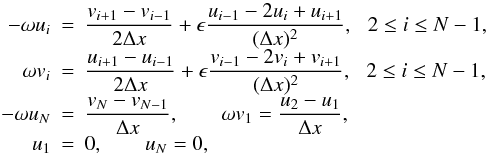 (14)where
ϵ is a free parameter ≪ 1. Although the order of the system has been
increased by 2, we did not include extra boundary conditions since this allows a smooth
transition between the case ϵ = 0 and ϵ ≠ 0, and is not
problematic from a numerical point of view. By choosing
ϵ = 2 × 10⁻³ (for N = 51), spurious
eigenvalues are removed from the interval ω ∈ [−18;18] , as is
displayed in Fig. 4 (second panel). We note that the
genuine eigenfunctions beyond this interval have a somewhat mixed character, as they are
influenced by the neighbouring spurious eigenfunctions, and are not always easy to
identify. Increasing the value of ϵ results in a larger interval
containing only genuine eigenmodes.
(14)where
ϵ is a free parameter ≪ 1. Although the order of the system has been
increased by 2, we did not include extra boundary conditions since this allows a smooth
transition between the case ϵ = 0 and ϵ ≠ 0, and is not
problematic from a numerical point of view. By choosing
ϵ = 2 × 10⁻³ (for N = 51), spurious
eigenvalues are removed from the interval ω ∈ [−18;18] , as is
displayed in Fig. 4 (second panel). We note that the
genuine eigenfunctions beyond this interval have a somewhat mixed character, as they are
influenced by the neighbouring spurious eigenfunctions, and are not always easy to
identify. Increasing the value of ϵ results in a larger interval
containing only genuine eigenmodes.
The main reason why this method works is because it introduces a second-order derivation
operator which is robust to mesh drift when expressed on the original grid, as opposed to
first-order derivation operators. To illustrate this point more clearly, we set up another
somewhat artificial system where the second-order operators are enforced on the midpoints
preceding the current grid points, whereas the other operators are enforced on the
original grid: 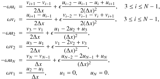 (15)The
associated eigenvalues are shown in Fig. 4 (third
panel), where ϵ = 2 × 10⁻³. This time no intervals containing
only genuine eigenmodes appear. If ϵ is further increased, the genuine
and spurious eigenmodes start to interact and form complex eigenpairs. One can also
calculate the basis functions of the null spaces associated with these two
second-derivative operators by applying the same procedure as in Sect. 2.2. The results are shown in Fig. 6. As expected, the first operator (upper panel) only has two basis
functions, both of which are affine functions (which are true solutions to the
mathematical problem). The second operator (lower panel) has a third basis function which
is highly oscillatory. If we reapply the same intuitive reasoning as earlier, we can
expect the second derivative of an oscillatory function to vanish near the inner midpoints
of a given window of grid points, hence the reason for this supplementary, oscillatory
basis function.
(15)The
associated eigenvalues are shown in Fig. 4 (third
panel), where ϵ = 2 × 10⁻³. This time no intervals containing
only genuine eigenmodes appear. If ϵ is further increased, the genuine
and spurious eigenmodes start to interact and form complex eigenpairs. One can also
calculate the basis functions of the null spaces associated with these two
second-derivative operators by applying the same procedure as in Sect. 2.2. The results are shown in Fig. 6. As expected, the first operator (upper panel) only has two basis
functions, both of which are affine functions (which are true solutions to the
mathematical problem). The second operator (lower panel) has a third basis function which
is highly oscillatory. If we reapply the same intuitive reasoning as earlier, we can
expect the second derivative of an oscillatory function to vanish near the inner midpoints
of a given window of grid points, hence the reason for this supplementary, oscillatory
basis function.
 |
Fig. 6 Null space basis functions for 2nd derivative operators enforced on the original grid (upper panel) and on the midpoints (lower panel). The functions (b1,b2...bD) are ordered such that the most oscillatory function comes first. |
An important drawback with this method is that it introduces a supplementary free parameter, ϵ, which needs to be carefully adjusted. On the one hand, if ϵ is too small, then the system will not be robust to mesh drift. On the other hand, a large value of ϵ alters the original system and reduces the overall accuracy. Another difficulty with this approach is that it is not always straightforward where and how to introduce the second-derivative operators. For instance, swapping the two terms proportional to ϵ in Eq. (14) is highly detrimental to the solutions and does not solve mesh drift. The reason for this behaviour is not obvious and is beyond the scope of this paper.
Another solution used for suppressing mesh drift consists in applying a staggered grid
approach. For instance, the variable u could be defined on the original
grid, and v on the midpoints. This would lead to the following difference
equations: 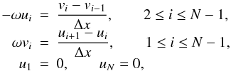 (16)where
we have assumed a uniform grid. The above system contains 2N − 3
difference equations and 2 boundary conditions for 2N − 1 unknowns. By
applying a QZ algorithm, we see that the spurious eigenvalues have once more been filtered
out (Fig. 4, fourth panel). The same mechanism which
filtered out mesh drift in the alternate grid approach also applies to the staggered grid
approach. However, the latter approach also comes with some disadvantages. Firstly,
there’s the inconvenience of having different variables defined on different grids.
Furthermore, if we had introduced, say, three variables in a 1D case, it is not entirely
clear which variables should be defined on what grids. If one defines the two first
variables on the original grid and the third one on the midpoints, they may be confronted
with a differential equation which relates the two first variables and which consequently
does not block mesh drift, since these variables are on the same grid (this may not be a
problem if the remaining equations are able to suppress mesh drift). Another solution
could consist in defining one of the variables on the original grid, a second one on the
one-third points, and the third one on the two-thirds points. However, such an approach
might be less effective at blocking mesh drift and certainly lacks the simplicity of using
the alternate grid approach. Another issue concerns the boundary conditions. If the
boundary conditions in Eq. (1) had been,
for example, u(0) + v(0) = 0 and
u(1) − v(1) = 0, then one needs to deal with the
values of both functions at both endpoints. However, the variable v is
defined on a grid which does not include the endpoints. As a result, some ad-hoc treatment
of the boundary conditions is required. Finally, as will be made clear in the following
section, the staggered grid approach does not always lend itself to superconvergence.
(16)where
we have assumed a uniform grid. The above system contains 2N − 3
difference equations and 2 boundary conditions for 2N − 1 unknowns. By
applying a QZ algorithm, we see that the spurious eigenvalues have once more been filtered
out (Fig. 4, fourth panel). The same mechanism which
filtered out mesh drift in the alternate grid approach also applies to the staggered grid
approach. However, the latter approach also comes with some disadvantages. Firstly,
there’s the inconvenience of having different variables defined on different grids.
Furthermore, if we had introduced, say, three variables in a 1D case, it is not entirely
clear which variables should be defined on what grids. If one defines the two first
variables on the original grid and the third one on the midpoints, they may be confronted
with a differential equation which relates the two first variables and which consequently
does not block mesh drift, since these variables are on the same grid (this may not be a
problem if the remaining equations are able to suppress mesh drift). Another solution
could consist in defining one of the variables on the original grid, a second one on the
one-third points, and the third one on the two-thirds points. However, such an approach
might be less effective at blocking mesh drift and certainly lacks the simplicity of using
the alternate grid approach. Another issue concerns the boundary conditions. If the
boundary conditions in Eq. (1) had been,
for example, u(0) + v(0) = 0 and
u(1) − v(1) = 0, then one needs to deal with the
values of both functions at both endpoints. However, the variable v is
defined on a grid which does not include the endpoints. As a result, some ad-hoc treatment
of the boundary conditions is required. Finally, as will be made clear in the following
section, the staggered grid approach does not always lend itself to superconvergence.
Rhie-Chow interpolation has also been frequently used to suppress mesh drift in fluid dynamics problems (Rhie & Chow 1983). This approach involves interpolating the velocity, using the momentum equation in which the pressure gradient has been replaced by a more stable expression only involving adjacent grid points. As a result, adjacent grid points become coupled, thereby suppressing mesh drift. This approach has the advantage of keeping all of the variables on the original grid, as opposed to the staggered grid approach. However, its main drawback is that it is specific to the momentum equation and doesn’t seem to have been extended into a general mathematical approach. Furthermore, it was originally developed using second-order finite-differences, and it is not clear whether it extends to higher orders.
4. Superconvergence
One last point of interest concerns the order of the finite-difference operators. In Eq. (12), the overall system has a second-order accuracy, whether or not the underlying grid is uniform. In Eq. (13), the overall accuracy is of third-order, in spite of having increased the window size from two to four. This is because, the derivation operators on the endpoints only locally achieve a second-order accuracy. Furthermore, if the underlying grid had been non-uniform, then the difference equations in the middle part of the domain would have been of third rather than fourth-order accuracy, when enforced on the midpoints. This is because, in general, finite differences calculated over a window of n grid points are accurate to order n − d, where d is the order of the derivative. However, the scheme used in Eq. (12) is an exception to this rule. Furthermore, Sadiq & Viswanath (2013) recently pointed out general conditions where the accuracy is boosted by one or several orders, a situation which they called “superconvergence”. This therefore raises the question as to whether such conditions can systematically be satisfied by carefully choosing the alternate grid on which to enforce the finite-difference scheme. In what follows, we show that the answer to this question is yes for an increase in accuracy by one order. We provide our own derivation of the condition for superconvergence and show that it is compatible with removing mesh drift. Our derivation is somewhat simpler than what is presented in Sadiq & Viswanath (2013) and leads to a formulation which is easily implemented numerically.
Let y be a function for which we’re seeking to approximate the
d-th derivative at a specified point, z, using finite
differences. Let
x1,x2...xn
be a set of n distinct grid points for which the function
y is known. A Taylor expansion centred on z of the
function y yields the following expression at each grid point
xi:
 (17)Finite-difference
coefficients
(17)Finite-difference
coefficients 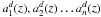 are then calculated so as to
satisfy:
are then calculated so as to
satisfy: 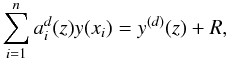 (18)where
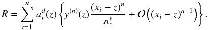 (19)This is achieved by having
the coefficients satisfy the following relationships:
(19)This is achieved by having
the coefficients satisfy the following relationships:
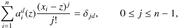 (20)where
δjd is Kronecker’s delta symbol. Despite
appearances, R is actually of order
(20)where
δjd is Kronecker’s delta symbol. Despite
appearances, R is actually of order  in most cases, where δx is representative of the separations between the
xi.
in most cases, where δx is representative of the separations between the
xi.
The goal is then to find z values for which the first part of
R cancels out:  (21)Finding such values
would guarantee that R is a least of order
(21)Finding such values
would guarantee that R is a least of order
 .
.
It turns out that the right hand side of Eq. (21) is a product of a polynomial of degree n − d
and of the nth derivative of y:  (22)where
 (23)It is straightforward to
see that the polynomial Q(d) has
n − d distinct zeros, which may be obtained by a
standard root solver. We also note, in passing, that Eq. (22) agrees with the first term of the Taylor expansion of the
finite-difference errors given in Bowen & Smith
(2005).
(23)It is straightforward to
see that the polynomial Q(d) has
n − d distinct zeros, which may be obtained by a
standard root solver. We also note, in passing, that Eq. (22) agrees with the first term of the Taylor expansion of the
finite-difference errors given in Bowen & Smith
(2005).
We start by calculating R for the function
y0(x) = xn.
Based on Eq. (18), one has:
 (24)According to Fornberg (1988), the coefficients
 are given by:
 (25)where
Li(z) is Lagrange’s
interpolation polynomial defined such that
Li(xj) = δij.
Let us define a polynomial P as follows:
(25)where
Li(z) is Lagrange’s
interpolation polynomial defined such that
Li(xj) = δij.
Let us define a polynomial P as follows:
 (26)It turns out that
P(d)(z) = R.
Furthermore:
(26)It turns out that
P(d)(z) = R.
Furthermore:  (27)However, P
is not identically zero but is of degree n, with a leading coefficient of
−1. From this, we deduce that P = −Q.
(27)However, P
is not identically zero but is of degree n, with a leading coefficient of
−1. From this, we deduce that P = −Q.
Based on its definition, Eq. (19),
R is also given by:
 (28)where we have used
 . Hence,
one obtains the following relationship:
. Hence,
one obtains the following relationship:
 (29)When inserted into the
right hand side of Eq. (21), this gives the
desired result, i.e. Eq. (22).
(29)When inserted into the
right hand side of Eq. (21), this gives the
desired result, i.e. Eq. (22).
If we now consider the case d = 1, the n − 1 roots of Q′ are interspersed with the n original grid points in the window. Enforcing the finite differences on the middle root (assuming n is even) therefore achieves the same result as using the midpoint in the middle, given that it stays far away from local extrema of an oscillatory function (see Fig. 3), and can consequently be expected to remove mesh drift. To verify this, we calculated the null space of a four-point derivation operator calculated for the non-uniform grid based on Eq. (3) and enforced on the middle root of Q′ (near the endpoints, the window size is reduced to three and we choose the root nearest the endpoints; however, this doesn’t intervene when calculating the null space). The basis functions of the null space are presented in the lower panel of Fig. 5 and display no oscillatory behaviour. If we return to our initial problem (Eq. (1)), spurious eigenvalues are once more filtered out (Fig. 4, last panel). Finally, in Fig. 7, we show the rate of convergence of the ω = π eigenvalue using the same non-uniform grid, and enforcing the finite differences on the midpoints and on the middle roots (dotted and continuous line, respectively). As expected, the error scales as N-3 when working with the midpoints and as N-4 when working with the middle roots.
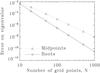 |
Fig. 7 Error on the ω = π eigenvalue of Eq. (1) as a function of the number of grid points, N. Using the roots of Q′ increases the rate of convergence from N-3 to N-4. |
At this point, it is fairly straightforward to see why the staggered grids approach does not always lend itself to superconvergence. Indeed, if we take our initial problem as an example, to achieve superconvergence the variable v needs to be defined on the root points of the grid associated with u, and vice-versa. This leads to two relationships between the two grids which are not necessarily compatible. If, for instance we consider two-point windows for simplicity, then the root points will coincide with the midpoints. To then achieve superconvergence, the midpoints of the midpoints of u’s grid need to coincide with the original grid points. This is only possible if the original grid is uniform.
5. Application to stellar pulsations
In practical situations, one will want to solve differential systems which are far more complicated than Eq. (1) and typically involve non-constant coefficients. As a result, to apply the above method, it will be necessary to interpolate these coefficients. This can easily be done, to the same order of accuracy, by simply reusing the same interpolation weights that were used on the variables. Also, in some situations, the underlying grid can be quite dense in areas where either the coefficients or the expected solutions vary rapidly. This can lead to poor results when calculating the roots of Q′. A simple remedy consists in applying an affine transformation to each window of grid points, in order to spread them out and recenter them around 0, before finding the roots of Q′. The inverse transformation then needs to be applied to the resultant roots, in order to obtain them with respect to the original grid. Although, both of these may represent extra complications compared to applying finite differences on the original grid points, the gain in numerical stability and accuracy makes this approach worthwhile.
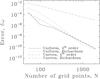 |
Fig. 8 Error on the frequency as a function of the grid resolution for a 2nd order approach combined with Richardson extrapolation and a 4th order approach, applied to uniform and uneven grids. |
We now demonstrate that the above approach can successfully be applied to stellar pulsations. In what follows we will apply an approach which uses four-point windows and superconvergence. Based on the preceding results, such an approach reaches fourth-order accuracy. In a first example, we focus on an acoustic mode in a polytropic stellar model and show this approach is both accurate and robust, even for a highly uneven grid, where Richardson extrapolation fails. In the second example, we apply this method to calculating oscillations in a realistic stellar model, namely Model S (Christensen-Dalsgaard et al. 1996) and show that it produces results in agreement with previous approaches and filters out spurious modes. Then we briefly describe how this approach is applied to 2D calculations of pulsation modes in rapidly rotating stars.
5.1. Richardson extrapolation on uneven grids
As a first example, we focus on the (n, ℓ) = (4,1) acoustic mode in an Np = 3 polytropic stellar model, were n is the radial order, ℓ the harmonic degree, and Np the polytropic index. We compare two approaches: the fourth-order scheme described above, and a second-order scheme supplemented with Richardson extrapolation. Two types of grids are considered: a uniform grid, and an uneven grid in which consecutive separations alternate between a large and a small value. The ratio of the small value to the large value has been set to 0.1.
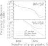 |
Fig. 9 Error on the frequencies of two modes as a function of the grid resolution for a 2nd order approach combined with Richardson extrapolation (implemented in the ADIPLS code) and a 4th order approach. The radial order, harmonic degree, and frequency of each mode is indicated in the upper right corner of each panel. |
Figure 8 then shows the error on the frequency, as a function of grid resolution, for both types of grids and finite-difference schemes. A fourth-order calculation using a uniform grid with 5001 points has been used to calculate the reference frequency used to evaluate the error (similar reference values are also obtained using Richardson extrapolation on the same grid, or using a spectral approach based on Chebyshev polynomials). When applying Richardson extrapolation, two calculations are carried out: one on the full grid, and one on a reduced version of the grid in which every other point is dropped out. Hence, the reduced version of the uneven grid turns out to be uniform, given that the grid-point separations alternate between a large and small value. As can be seen in the figure, Richardson extrapolation leads to fourth-order accuracy for the uniform grid but not the uneven grid. Indeed, the second-order errors have not been removed in the latter case. In contrast, the fourth-order scheme yields fourth-order accuracy, regardless of the grid. Of course, one must bear in mind that this situation is somewhat contrived and that the underlying grids used in most stellar pulsation calculations are close to uniform over short intervals, even if they are highly uneven over the entire domain. Hence, in most practical situations, Richardson extrapolation will improve results and lead to near fourth-order accuracy.
 |
Fig. 10 Frequency spectrum of ℓ = 1 modes calculated in Model S (interpolated onto 1001 grid points) using a QZ algorithm. Spurious modes only appear at the outskirts of the spectrum where the numerical resolution is insufficient to resolve the modes. |
5.2. Model S
In order to test the above scheme in a more realistic situation, we apply it to calculating stellar pulsations in Model S, a reference model representative of the current Sun (Christensen-Dalsgaard et al. 1996). This model is interpolated onto grids of different resolutions (N = 51, 101, 201, 501, ... 10 001) using the program redistrb.d which comes with the ADIPLS package. The option appropriate for p-modes was selected thereby causing the underling grid to be dense near the surface where the sound velocity, and hence the wavelength, is small. A simple surface boundary condition δp = 0 was used when calculating the pulsation modes.
Figure 9 shows the errors on the frequencies of two modes as a function of the grid resolution. The second-order calculation supplemented with Richardson extrapolation was carried out using the ADIPLS code (?). The upper and lower panels correspond to low and high frequency acoustic modes, respectively. For each method, the errors on the frequencies were calculated using the frequency calculation at 10 001 points, for that particular method, as a reference value. These errors are shown as dotted and dashed lines for the fourth-order method, and the second-order method with Richardson extrapolation, respectively. Finally, the solid line indicates the frequency differences between both methods. For the low frequency mode, the differences between both methods is very small and comparable to the errors on the frequencies. We note, however, that the general slope of the errors is closer to N-2 rather than N-4, regardless of the method. A possible reason for this may be the way the model is interpolated onto the different grids. The situation is different for the high frequency mode. This time the slope of the error is close to N-4, as expected theoretically. However, as shown by the solid line, the two methods converge to values approximately 8 nHz apart, which is substantially larger than what was obtained for the low frequency mode. Nonetheless, this remains smaller than the difference between the variational and Richardson frequencies (approximately 58 nHz). Hence, these two methods agree to a high degree of accuracy, thereby validating the fourth-order approach in a realistic situation.
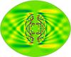 |
Fig. 11 Meridional cross-section of a pulsation mode in a stellar model rotating at 70% of the critical break-up rotation rate. This mode was calculated using the fourth-order scheme with superconvergence in the radial direction and a spectral method based on spherical harmonics in the angular direction. The resolution is 1601 radial grid points and 40 spherical harmonics. |
A second test consisted in numerically calculating an entire ℓ = 1 pulsation spectrum for the N = 1001 model, using a QZ algorithm. The QZ algorithm is an iterative procedure for finding all of the solutions of the generalised eigenvalue problem Ax = λBx where A and B are general square matrices (Moler & Stewart 1973). The implementation we used comes from the LAPACK3 linear algebra library. Figure 10 shows parts of the frequency spectrum which include the first hundred p and g modes. A mixture of both real and complex eigenvalues appear. Given that the pulsation calculations are based on the adiabatic approximation, the complex eigenvalues can only be due to numerical artifact, and must be considered as spurious. However, these solutions are located at the outskirts of the frequency spectrum, i.e. where modes are unresolved due to insufficient grid resolution. In contrast, an inspection of the modes with −100 ≤ n ≤ 100 did not reveal spurious modes, complex eigenvalues, or mesh drift. We therefore conclude that this method has successfully removed the problems related to mesh drift.
5.3. 2D calculations in rapidly rotating stars
The fourth-order approach has also been successfully applied to calculating pulsation modes in rapidly-rotating centrifugally-distorted stars, a far more complicated eigenvalue problem involving 2D partial differential equations. Indeed, it has been used for the radial discretisation in the TOP code and represents a definite improvement over the unstable scheme previously used in Reese et al. (2009). Based on this improvement, Burke et al. (2011) obtained stable numerical behaviour when calculating the pulsations of centrifugally-deformed models from the ASTEC code (?), and Reese et al. (2013) were able to remove spurious modes from the pulsation spectra of models based on the Self-Consistent Field (SCF) Method (MacGregor et al. 2007), which is important when scanning an entire spectrum. As an example, Fig. 11 shows the meridional cross-section of a rosette mode (Ballot et al. 2012) in an SCF stellar model, using this approach.
6. Conclusion
In this paper, we have explored different ways of setting up higher order finite difference schemes for calculating stellar pulsations. This lead us to investigating mesh drift and related problems, such as spurious modes. After having illustrated and characterised mesh drift, we proposed a simple remedy which furthermore lends itself to “superconvergence”, a way of boosting the order of accuracy of finite differences by one. We then applied this method to 1D and 2D stellar pulsation calculations, and showed that it was accurate, flexible with respect to underlying grid, and able to remove to mesh drift. Finally, we should emphasise that although this approach was specifically developed for calculating stellar pulsations, it is easily applicable and beneficial to many other physical or mathematical problems.
Orthogonal with respect to the dot product
f·g = ∑ ifigi.
This implies that that the basis elements will be normalised as follows:
 .
.
Initially, this basis will be expressed in terms of the reduced coordinates
(μj) but can easily be re-expressed over
the initial grid using the elements of .
Orthogonality of the resultant basis follows from that of the basis expressed in terms of
the reduced coordinates.
We specifically used the DGGEV routine, which is based on the DHGEQZ routine. LAPACK is available at http://www.netlib.org/lapack/
Acknowledgments
DRR thanks the referee, Michel Rieutord, and François Lignières for useful comments and suggestions which have improved and clarified the manuscript. DRR is financially supported through a postdoctoral fellowship from the “Subside fédéral pour la recherche 2011”, University of Liège, and was previously supported by the CNES (“Centre National d’Études Spatiales”), both of which are gratefully acknowledged.
References
- Ballot, J., Lignières, F., Prat, V., Reese, D. R., & Rieutord, M. 2012, in Progress in Solar/Stellar Physics with Helio- and Asteroseismology, eds. H. Shibahashi, M. Takata, & A. E. Lynas-Gray, ASP Conf. Ser., 462, 389 [Google Scholar]
- Bowen, M. K., & Smith, R. 2005, Proc. Roy. Soc. A, 461, 1975 [NASA ADS] [CrossRef] [Google Scholar]
- Brassard, P., & Charpinet, S. 2008, ApSS, 316, 107 [NASA ADS] [Google Scholar]
- Brassard, P., Pelletier, C., Fontaine, G., & Wesemael, F. 1992, ApJS, 80, 725 [NASA ADS] [CrossRef] [Google Scholar]
- Burke, K. D., Reese, D. R., & Thompson, M. J. 2011, MNRAS, 414, 1119 [NASA ADS] [CrossRef] [Google Scholar]
- Christensen-Dalsgaard, J. 2008a, ApSS, 316, 113 [NASA ADS] [Google Scholar]
- Christensen-Dalsgaard, J. 2008b, ApSS, 316, 13 [NASA ADS] [Google Scholar]
- Christensen-Dalsgaard, J., Dappen, W., Ajukov, S. V., et al. 1996, Science, 272, 1286 [CrossRef] [Google Scholar]
- Dupret, M. A. 2001, A&A, 366, 166 [NASA ADS] [CrossRef] [EDP Sciences] [Google Scholar]
- Dupret, M.-A., Belkacem, K., Samadi, R., et al. 2009, A&A, 506, 57 [NASA ADS] [CrossRef] [EDP Sciences] [Google Scholar]
- Fornberg, B. 1988, Math. Comp., 51, 699 [CrossRef] [MathSciNet] [Google Scholar]
- Gautschy, A., & Glatzel, W. 1990, MNRAS, 245, 154 [Google Scholar]
- Kreiss, H.-O. 1978, Numerical Methods for Solving Time-Dependent Problems for Partial Differential Equations (Montreal, Canada: University of Montreal Press), 66 [Google Scholar]
- MacGregor, K. B., Jackson, S., Skumanich, A., & Metcalfe, T. S. 2007, ApJ, 663, 560 [NASA ADS] [CrossRef] [Google Scholar]
- Moler, C. B., & Stewart, G. W. 1973, SIAM J. Num. Anal., 10, 241 [Google Scholar]
- Moya, A., Christensen-Dalsgaard, J., Charpinet, S., et al. 2008, ApSS, 316, 231 [Google Scholar]
- Press, W. H., Teukolsky, S. A., Vetterling, W. T., & Flannery, B. P. 2007, Numerical Recipes 3rd edn., The Art of Scientific Computing (New York, NY, USA: Cambridge University Press) [Google Scholar]
- Reese, D., Lignières, F., & Rieutord, M. 2006, A&A, 455, 621 [NASA ADS] [CrossRef] [EDP Sciences] [Google Scholar]
- Reese, D. R., MacGregor, K. B., Jackson, S., Skumanich, A., & Metcalfe, T. S. 2009, A&A, 506, 189 [NASA ADS] [CrossRef] [EDP Sciences] [Google Scholar]
- Reese, D. R., Prat, V., Barban, C., van ’t Veer-Menneret, C., & MacGregor, K. B. 2013, A&A, 550, A77 [NASA ADS] [CrossRef] [EDP Sciences] [Google Scholar]
- Rhie, C. M., & Chow, W. L. 1983, AIAA Journal, 21, 1525 [Google Scholar]
- Richardson, L. F., & Gaunt, J. A. 1927, Philosophical Transactions of the Royal Society of London, Series A, 226, 299 [Google Scholar]
- Roxburgh, I. W. 2008, ApSS, 316, 141 [Google Scholar]
- Sadiq, B., & Viswanath, D. 2013, Math. Comp. [arXiv:1102.3203] [Google Scholar]
- Scuflaire, R., Montalbán, J., Théado, S., et al. 2008, ApSS, 316, 149 [Google Scholar]
- Takata, M., & Löffler, W. 2004, PASJ, 56, 645 [NASA ADS] [Google Scholar]
- Valsecchi, F., Farr, W. M., Willems, B., & Kalogera, V. 2013, ApJ, accepted [arXiv:1301.3197] [Google Scholar]
All Figures
|
Fig. 1 Spurious numerical solutions to Eq. (1) caused by mesh drift, using a 2nd order finite-difference scheme on a uniform grid (upper panel), a 4th order scheme on a uniform grid (middle panel), and a 2nd order scheme on a non-uniform grid. The number of grid points, N, is indicated in the upper right corner of each panel. |
| In the text | |
|
Fig. 2 Null space basis functions for the finite-difference schemes used in Fig. 1 (except that the resolution has been reduced for the sake of legibility). The functions (b1,b2...bD) are ordered such that the most oscillatory function comes first. |
| In the text | |
|
Fig. 3 An oscillatory function (represented by the “ × ”) and its interpolating polynomial (represented by the continuous line), defined over a slightly non-uniform 5-point window. |
| In the text | |
|
Fig. 4 Eigenvalues with positive real parts obtained with a QZ algorithm for various finite-difference schemes. The labelling of the eigenvalues is based on a visual inspection of the corresponding eigenmodes. The shaded grey area corresponds to solutions which are not fully resolved – we required approximately 8 points per oscillation period of the genuine solutions (in the sixth panel, this area is larger simply because we used a non-uniform grid). In all cases, the resolution is N = 51. |
| In the text | |
|
Fig. 5 Null space basis functions for finite-difference schemes enforced on alternate grids (midpoints and roots). The functions (b1,b2...bD) are ordered such that the most oscillatory function comes first. |
| In the text | |
|
Fig. 6 Null space basis functions for 2nd derivative operators enforced on the original grid (upper panel) and on the midpoints (lower panel). The functions (b1,b2...bD) are ordered such that the most oscillatory function comes first. |
| In the text | |
|
Fig. 7 Error on the ω = π eigenvalue of Eq. (1) as a function of the number of grid points, N. Using the roots of Q′ increases the rate of convergence from N-3 to N-4. |
| In the text | |
|
Fig. 8 Error on the frequency as a function of the grid resolution for a 2nd order approach combined with Richardson extrapolation and a 4th order approach, applied to uniform and uneven grids. |
| In the text | |
|
Fig. 9 Error on the frequencies of two modes as a function of the grid resolution for a 2nd order approach combined with Richardson extrapolation (implemented in the ADIPLS code) and a 4th order approach. The radial order, harmonic degree, and frequency of each mode is indicated in the upper right corner of each panel. |
| In the text | |
|
Fig. 10 Frequency spectrum of ℓ = 1 modes calculated in Model S (interpolated onto 1001 grid points) using a QZ algorithm. Spurious modes only appear at the outskirts of the spectrum where the numerical resolution is insufficient to resolve the modes. |
| In the text | |
|
Fig. 11 Meridional cross-section of a pulsation mode in a stellar model rotating at 70% of the critical break-up rotation rate. This mode was calculated using the fourth-order scheme with superconvergence in the radial direction and a spectral method based on spherical harmonics in the angular direction. The resolution is 1601 radial grid points and 40 spherical harmonics. |
| In the text | |
Current usage metrics show cumulative count of Article Views (full-text article views including HTML views, PDF and ePub downloads, according to the available data) and Abstracts Views on Vision4Press platform.
Data correspond to usage on the plateform after 2015. The current usage metrics is available 48-96 hours after online publication and is updated daily on week days.
Initial download of the metrics may take a while.