| Issue |
A&A
Volume 554, June 2013
|
|
|---|---|---|
| Article Number | A22 | |
| Number of page(s) | 11 | |
| Section | The Sun | |
| DOI | https://doi.org/10.1051/0004-6361/201220738 | |
| Published online | 30 May 2013 | |
Collisions, magnetization, and transport coefficients in the lower solar atmosphere
1 R. Vandervaerenlaan 16/402, 3000 Leuven, Belgium
e-mail: This email address is being protected from spambots. You need JavaScript enabled to view it.
2 Institute of Physics Belgrade, Pregrevica 118, 11080 Zemun, Serbia
3 Joint Institute of Computational Sciences, University of Tennessee, Oak Ridge, TN 37831-6173, USA
e-mail: This email address is being protected from spambots. You need JavaScript enabled to view it.
Received: 15 November 2012
Accepted: 5 April 2013
Abstract
Context. The lower solar atmosphere is an intrinsically multi-component and collisional environment with electron and proton collision frequencies in the range 108−1010 Hz, which may be considerably higher than the gyro-frequencies for both species. Collisions between different species are altitude dependent because of the variation in density and temperature of all species.
Aims. We aim to provide a reliable quantitative set of data for collision frequencies, magnetization, viscosity, and thermal conductivity for the most important species in the lower solar atmosphere. Having such data at hand is essential for any modeling that is aimed at describing realistic properties of the considered environment.
Methods. The relevant elastic and charge transfer cross sections in the considered range of collision energies are now accepted by the scientific community as known with unprecedented accuracy for the most important species that may be found in the lower solar atmosphere. These were previously calculated using a quantum-mechanical approach and were validated by laboratory measurements. Only with reliable collision data one can obtain accurate values for collision frequencies and coefficients of viscosity and thermal conductivity.
Results. We describe the altitude dependence of the parameters and the different physics of collisions between charged species, and between charged and neutral species. Regions of dominance of each type of collisions are clearly identified. We determine the layers within which either electrons or ions or both are unmagnetized. Protons are shown to be unmagnetized in the lower atmosphere in a layer that is at least 1000 km thick even for a kilo-Gauss magnetic field that decreases exponentially with altitude. In these layers the dynamics of charged species cannot be affected by the magnetic field, and this fact is used in our modeling. Viscosity and thermal conductivity coefficients are calculated for layers where ions are unmagnetized. We compare viscosity and friction and determine the regions of dominance of each of the phenomena.
Conclusions. We provide the most reliable quantitative values for most important parameters in the lower solar atmosphere to be used in analytical modeling and numerical simulations of various phenomena such as waves, transport and magnetization of particles, and the triggering mechanism of coronal mass ejections.
Key words: Sun: photosphere / Sun: chromosphere / Sun: fundamental parameters
© ESO, 2013
1. Introduction
There has recently been a considerable shift of focus of solar researchers from ideal and collision-less toward collisional phenomena in the solar atmosphere (e.g., Arber et al. 2007; Pandey & Wardle 2008; Soler et al. 2010; Barceló et al. 2011; Zaqarashvili et al. 2011a,b; Khomenko & Collados 2012). This is understandable for lower atmosphere layers because this is a partially ionized medium with several species whose dynamics is heavily coupled and affected by mutual collisions and by collisions between similar particles (Vranjes & Poedts 2006a; Vranjes et al. 2007; 2008a). In some layers of the photosphere the ion-neutral and electron-neutral collision frequencies are approximately 109 and 1010 Hz, respectively. This makes both ions and electrons in these layers very weakly magnetized or completely unmagnetized.
In recent multi-component models in the literature, the medium has typically been treated as if it consisted of two components, neutrals and “plasma”. These models consequently neglected differences between electron and ion dynamics, similarly to ordinary magneto-hydrodynamics theory. However, in the lower solar atmosphere it is very difficult to justify this approach, as we show below. One reason for this are the different collision frequencies of electrons and ions, which among other effects imply different magnetization of these two species, consequently producing quite different effects of the magnetic field on particle dynamics.
The key components in the lower solar atmosphere are identified in the present work. We also show their collision cross sections and collision frequencies as a function of altitude. Using these results, the altitude-dependent magnetization of electrons and ions, the viscosity tensor, and the thermal conductivity vector components are calculated. The altitude-dependence of the parameters is presented graphically.
2. Key ingredients
The lower solar atmosphere is an essentially multi-component system that includes electrons, protons, neutral hydrogen H and helium He atoms, helium ions He+ or/and He++ etc. The dissociation energy of molecular hydrogen H2 is ≃4.5 eV and its presence may be expected throughout the lower solar atmosphere. However, recent observations (Jaeggli et al. 2012) showed that the regions with the highest amount of molecular hydrogen are sunspots where the total fraction of H2 molecules may reach a few percent only. On the other hand, the ionization energy of the hydrogen molecule, 15.603 eV, exceeds the ionization energy of atomic hydrogen, so the presence of the ionized hydrogen molecule is most likely negligible. Having in mind all possible collisional combinations of various particles, it is essential to identify the most important of their interactions before making any attempt to obtain realistic models for wave damping, diffusion, transport, magnetization of particles, etc. The collision cross sections can vary with the energy of colliding particles, which in the solar atmosphere is equivalent to the variation of the temperature with altitude.
Detailed studies available in the literature (Krstic & Schultz 1998; Glassgold et al. 2005; Schultz & Krstic 2008; Jamieson et al. 2000, and others) show large differences between the cross sections describing collisional phenomena such as elastic scattering, momentum transfer, viscosity, spin exchange, and charge exchange. Among these the most prevalent is typically the elastic scattering. Physically, this cross section should be taken into account in estimating the magnetization. On the other hand, the cross section for momentum transfer should be used in calculating friction; this type of cross section turns out to be usually lower than the elastic scattering. Knowing these details may be essential in realistic modeling of the lower solar atmosphere.
One also needs to include some inelastic collisions, which clearly may play a decisive role in the partially ionized solar atmosphere (Vranjes & Poedts 2006b), which makes the whole analysis significantly more complicated. These processes are the radiative recombination (of the type A+ + e → A + hν), three-body recombination (of the type A+ + e + e → A + e), dissociative recombination (e.g. of the type  , where A∗ is an excited atom), ionization by electron impact (the process of the type A + e → A+ + e + e), the ion-atom (or molecule) interchange reactions of the type A+ + BC → (AB)+ + C, etc.
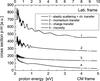 |
Fig. 1 Integral cross sections σpH for proton (p) collisions with neutral hydrogen atoms H for quantum-mechanically indistinguishable nuclei of the projectile and target particles, following Krstic & Schultz (1998). Here and throughout the text 1 a.u. = 2.8 × 10⁻²¹ m2, 1 eV ≃ 11 604 K. |
The presence of inelastic collisions implies modifications of equations through appropriate source/sink terms that appear in the continuity equation, in the momentum and in the energy equations. Only collisional phenomena from the first group mentioned above, i.e., elastic and charge transfer processes, are discussed here. Even then, as will become evident in the following sections, we still encounter a plethora of processes that could further be classified by priority and dominance to perform any meaningful analysis.
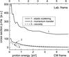 |
Fig. 2 Integral cross sections σpHe for proton collisions with neutral helium He. |
There exists a numerous literature dealing with collisional plasmas in the laboratory environment. The laboratory knowledge is in principle directly applicable to the relevant phenomena in the solar atmosphere. However, we find that i) the theoretical and experimental results are scattered to a large extent, and; ii) for the purpose of solar plasma studies, the cross sections for a specific range of parameters of the solar plasma are missing. For this reason we present cross sections for possible key-players in the lower solar atmosphere in the following subsection, with the energies of colliding particles in the range appropriate for the plasma below the transition region. These results, combined with the existing models of the altitude-dependent densities and temperature of the plasma species, are the essential and sufficient ingredients for calculating collision frequencies that are necessary for modeling.
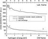 |
Fig. 3 Integral cross section σHH for collisions between neutral hydrogen atoms H for quantum-mechanically indistinguishable nuclei. |
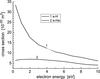 |
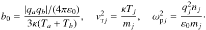
Fig. 4 Cross section for elastic scattering of electrons on neutral hydrogen atoms H and neutral helium atoms He, in terms of the electron energy. |
2.1. Cross sections for charge-neutral and neutral-neutral collisions
Figures 1–4 described in this section provide cross sections for all most important ingredient species in the lower atmosphere, given in terms of the energy (temperature) of the colliding species, which makes them directly applicable to the varying temperature with the altitude. The cross section profiles in Figs. 1–3 are based on works of Krstic & Schultz (1998; 1999a,b). These authors derived both differential and integral cross sections for elastic scattering. The cross sections for the momentum transfer and viscosity are the first and second moments of these (see also Dalgarno et al. 1958; Hasted 1964; Brandsen 1970; Makabe & Petrovic 2006; Schunk & Nagy 2009). In the first (momentum transfer) the differential elastic cross section is weighted by a scattering angle θ dependent term, 1 − cosθ, while in the second (viscosity) it is weighted by sin2θ. These weighting factors describe different features associated with momentum transfer and viscosity. For the viscosity this emphasizes the scattering at an angle π/2 and de-emphasizes the forward and backward ones. Scattering to such large angles is very effective in equalizing energies of the colliding particles. This is seen from the expressions for energies of the two particles before (E1, E2) and after collisions ( ,
,  ) in the laboratory frame, expressed through their total energy E in the laboratory frame and scattering angle θ in the CM frame:
  ,
, 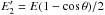 . Hence, such large-angle scattering tends to reduce both viscosity and conductivity. On the other hand, the factor 1 − cosθ in the momentum transfer cross section emphasizes the backward-scattering angles, and this cross section determines the average momentum lost in collisions. Note also that charge exchange is a backward-scattering process. Many more details on these cross sections can be found in Krstic & Schultz (1998; 1999b), currently the most accurate cross sections for elastic processes and resonant charge transfer. The energy range in Figs. 1–3 in the center of mass (CM) of colliding particles is 0.1–5 eV (bottom x-axis), while in the laboratory (plasma) frame the energy range is given by the top x-axis using the transformation formula Elab = ECM(m1 + m2)/m2, where m2 is the mass of the target particle, and 1 a.u. = 2.8 × 10⁻²¹ m2, 1 eV ≃ 11 604 K.
We start with the cross sections for proton collisions with neutral hydrogen (p-H), shown in Fig. 1. They are based on quantum-mechanical indistinguishability of the projectile and target nuclei (Krstic & Schultz 1998). The elastic scattering curve from Fig. 1 (line 1) was used to calculate magnetization, i.e., for the ratio of the collision frequency and the gyro-frequency of protons. It is the sum of the pure elastic scattering cross section and the charge transfer cross section. In estimating the friction caused by neutral hydrogen, it is appropriate to use the momentum transfer cross section (line 2). The amplitude oscillations of the cross sections are the consequence of quantum effects, which are present only at lowest collision energies (in the present study this means throughout the photosphere and chromosphere).
We stress that when one approximates the distinguishable particles, the elastic scattering cross sections and their higher momenta (momentum transfer and viscosity) are lower. This is because in this case we assume that we can distinguish between elastically and charge-transfer scattered protons, resulting in a separate treatment of these processes. When these particles cannot be distinguished, as is the case at lowest energies (lower than 1 eV), the elastic cross sections of the indistinguishable particles and their moments are the coherent sum of the processes, elastic and charge transfer. For indistinguishable nuclei, the integral elastic cross section together with the charge transfer at 0.2,0.5,1 eV in the CM frame is, 788.660,679.534, and 582.292 a.u., while the distinguishable nuclei model yields 598.068, 506.701, and 419.739 a.u. Similar holds for the momentum transfer, while the charge transfer cross section is practically the same for both models. One has to have in mind these differences and the differences in the physical definitions of these cross sections, to avoid twice counting elastic and charge transfer cross sections: the elastic cross section of the indistinguishable particle and their moments in Fig. 1 already contain both processes.
In Fig. 2 the three lines describe the collisions between protons and neutral helium atoms. Observe that the momentum transfer and viscosity lines are below the line for elastic scattering by a factor 4–5. This is because the momentum transfer presents the differential cross sections in the backward-scattering directions, while the dominant contribution in the elastic cross sections comes form the forward-scattering angles, which dominate the differential elastic cross sections. Therefore, for the proton dynamics the presence of neutral helium may be more important for estimating magnetization than for the momentum loss caused by friction or by viscosity (as compared to those that come from proton self-collisions or interaction with hydrogen, see more in Sect. 6).
Figure 3 gives collision cross sections between neutral hydrogen atoms according to Krstic & Shultz (1998). The momentum transfer and elastic collisions curves coincide, and line 1 in the two figures describes the most dominant interaction for the solar atmosphere. Note that it includes both direct and recoil scattering as a direct consequence of the indistinguishability of particles, and the same holds for the viscosity cross section. Due to these reasons the presented values are twice as high as the classic values obtained from the model of distinguishable particles.
The new type of cross section that appears in Fig. 3 is the spin exchange cross section, which describes collisions in which electrons (from the two colliding atoms) with different spin orientation are exchanged. Processes of this type are the reason for the cooling phenomena in the upper atmosphere, interplanetary space, and galactic HI regions (Bates 1951; Purcell & Field 1956; Dalgarno 1961).
Observe the difference between the lines 1 in Fig. 1 and in Fig. 3. One obvious reason for this is the charge transfer cross section, which is contained in line 1 in Fig. 1. This can be subtracted to obtain the pure elastic scattering value σel,pH. The cross section obtained in this way, at high energies, tends smoothly toward the corresponding elastic cross section obtained from the classic model of distinguishable particles. At the low energies of interest here, 0.5 and 1 eV (in CM frame), this yields σel,pH = 507.333,420.038 a.u. as the pure elastic scattering cross section for p-H collisions. For the H-H collisions in Fig. 3 the corresponding values are lower by about 137 and 81 a.u. for the two energies, respectively. The difference that still remains (i.e., greater p-H than H-H cross section) should be attributed to the fact that proton collision with H atoms causes charge polarization on the neutral atom (see Chen & Chang 2003; and in Vranjes et al. 2002). This means that to some extent p-H collisions involve features of the Coulomb interaction. The physics behind this is as follows: a point charge q0 placed at some distance from an atom with the radius a that has a point positive charge q in the core and uniform negative cloud − q around it, will cause displacement of the initially uniform cloud charge. If the external point charge q0 is an electron, this displacement is in the direction away from the electron position. If the external point charge q0 is a positive ion, this displacement of the cloud charge will be toward the ion and the force will again be attractive. The energy from this attractive Coulomb interaction according to Chen & Chang (2003) is 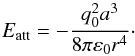 (1)Hence, collisions of charged species with neutrals indeed involve a Coulomb-type interaction, which affects collisions at very short distances, see also Dalgarno et al. (1958) and McDowell & Coleman (1970).
Finally, we give plot in Fig. 4 with three lines for the cross sections for the electron scattering on the two most important atoms hydrogen H and neutral helium atoms He in the electron energy range 0.1–10 eV. The lines represent some mean values from many references, see for example Bedersen & Kieffer (1971) and references cited therein. The possible uncertainty is almost 10–25 percent at low energies. This also agrees with some other sources, for instance Brode (1933), Brackmann et al. (1958), Kieffer (1971), Mitchner & Kruger (1973), Tawara et al. (1990), and Fortov et al. (2006). Hence, although some uncertainty for electron cross sections exists, it is not substantial. Clearly, at the low energies of interest for photosphere and chromosphere the most probable are electron collisions with atomic hydrogen H. We investigate the electron Coulomb collisions in the following section.
3. Electron collision frequencies
To describe the collisions between charged particles we use the following expression for the collision frequency between the charged species b and a following Spitzer (1962) and Vranjes et al. (2008b): 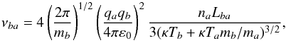 (2)
(2)
![Mathematical equation: $$ L_{ba}=\log[r_d/b_0],\quad r_d=\frac{r_{da} r_{db}}{(r_{da}^2 + r_{db}^2)^{1/2}}, \quad r_{dj}= \frac{v_{{\rm \sss T} j}}{\omega_{{\rm p}j}}, $$](/articles/aa/full_html/2013/06/aa20738-12/aa20738-12-eq55.png)
 As is well known, the Coulomb logarithm Lba (introduced by Spitzer) describes the cumulative effect of numerous small angle deflections that are intrinsic to Coulomb-type collisions.
These expressions are used to calculate collisions for electrons for the parameters (density and temperature) that vary with altitude, The results are presented in Fig. 5. To incorporate the variation of the parameters, here and throughout the text we use the values given in Table C in Fontenla et al. (1993).
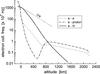 |
Fig. 5 Electron collisions with the altitude. For comparison, the thin line gives the electron gyro-frequency Ωe for the starting value of the magnetic field B0 = 0.1 T. |
For electron collisions with neutrals we read the cross sections σ(x) from Fig. 4, and then calculate the collision frequency using the expression 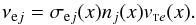 (3)The small differences of the parameters (density and temperature) given in the reference above, as compared with some other models of the lower solar atmosphere from the same authors or others, are of no particular importance for the general picture that is obtained.
The same holds for the expression νej used here in comparison with some modifications of it that may be seen in the literature. For example, the thermal speed we use is without any numerical parameter, as for the mean velocity v = [8κT/(πmab)] 1/2, mab = mamb/(ma + mb), which is sometimes used in the literature. It is easily seen that in the most drastic case, for example when a = b, this increases our thermal speed by a factor 2.2 only. Similar numerical parameters appear in the most probable speed v = (2κT/m)1/2, and in the root-mean-square velocity  . However, these modifications are not substantial in view of our much more accurate cross sections as compared with those that are typically used in the solar plasma literature (see comments in Sect. 7).
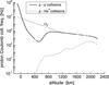 |
Fig. 6 Coulomb collisions of protons in terms of altitude. |
The electron collision frequency was checked also for e-He+ collisions. For the given altitude range the maximum e-He+ collision frequency is at about x = 2000 km altitude, but it is only 0.02 (in the same units as in Fig. 5) and is therefore completely negligible. After checking for the electron collision frequency with He++ ions we found out that it was even lower, at least by one order of magnitude.
The electron collisions with neutral helium He are even lower than the dominant collisions in Fig. 5. For example, at x = 0 we have νeHe = 2.2 × 10⁸ Hz, which is almost two orders below νeH, and it remains well below in the whole region.
Figure 5 suggests that in the region 0–850 km the electrons’ collisions with atomic hydrogen are by at least two orders of magnitude more frequent than the electron-electron collisions. Above 850 km e-p collisions (and the associated friction) should be more important than both e-e collisions and electron collisions with neutrals. Below the level denoted by x = 0 the Coulomb collisions become more dominant.
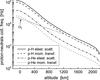 |
Fig. 7 Collision frequency for protons colliding with the neutral atoms H and He. |
According to Table C in Fontenla et al. (1993), at 850 km altitude the proton and H number densities are about 1017 m-3 and 1020 m-3, respectively, i.e., neutral hydrogen atoms are about 1000 times more abundant, yet e-p collisions are already more frequent. A similar situation is observed in the interval between x = − 100 km and x = 0. Here and throughout the negative altitude denotes the value below the referent level x = 0, i.e., toward the center of the Sun. This all confirms the well-known fact that the Coulomb collisions have a much larger cross section and are more frequent even in rather weakly ionized plasmas (see in Ratcliffe 1959; Vranjes & Poedts 2008). These facts are frequently overlooked in the literature.
4. Proton collision frequencies
Proton collision frequencies νpj where j includes protons as well as other relevant charged or neutral species are presented in Figs. 6 and 7. Here, for proton-neutral collisions we have νpj = σpjnjvTi and σpj is given in Figs. 1 and 2 in lines 1 and 2. In Fig. 6 the Coulomb p-p and p-He+ collision frequencies are presented using Eq. (2). Although p-He+ collisions are obviously much less frequent, their actual importance may be understood only by comparing the friction and viscosity terms in the momentum equation, see Sect. 6.
In Fig. 7, the cross section σ(x) = σ(T(x)) is obtained from Figs. 1 and 2 for the energies in the plasma frame (i.e., those given by the top x-axes), and the density and temperature (energy) from Table C in Fontenla et al. (1993).
Comparing Figs. 6 and 7, clearly proton collisions with neutral hydrogen are by far the most dominant in the given range (which starts from x = −100 km) up to the altitude of about 1350 km (there is a difference of almost four orders of magnitude for collisions in certain lower layers). Above 1350 km the amount of neutrals is sufficiently reduced so that p-p collisions become dominant. The highest proton collision frequencies at x = −100 km read νpH = 2 × 10⁹ Hz, νpp = 7 × 10⁸ Hz, νpHe = 8 × 10⁷ Hz.
Above 1900 km proton collisions with He+ are more frequent than p-H, which is even more true for p-He collisions. For example, at x = 2017 km we have νpHe+ = 3.3 × 10³ Hz (see Fig. 6), while νpH = 1.2 × 10³ Hz and νpHe = 62 Hz (see Fig. 7), and higher up this difference increases. Accordingly, above this layer proton friction with (any) neutral atoms is negligible.
5. Electron and proton magnetization
To estimate the magnetization, the thin line in Fig. 5 gives the electron gyro-frequency Ωe(x) = eB0(x)/me for a starting value of the magnetic field B0 = 0.1 T which approximately changes exponentially with the altitude as exp [ − x/(2h)], h = 125 km, following the thin-flux tube model and the usual pressure balance conditions. In the region below x = 0 the Coulomb collisions (e-p and e-e) become more dominant (see Fig. 5), and clearly the collision frequency in that area is higher than the electron gyro-frequency even for B0 = 0.1 T. Hence, in this layer νe/Ωe > 1 and electron dynamics should not be influenced by the magnetic field (see also Vranjes et al. 2007).
The layer without magnetization is much wider for protons and other ions. The corresponding line for protons is given in Figs. 6 and 7. For the same exceptionally strong starting field B0 = 0.1 T we have Ωi ≃ 9.6 MHz, which changes with altitude in such a way that it remains below νpH up to at least 1000−1200 km. Above this altitude the magnetic canopy is formed and the field changes less rapidly; it is therefore expected that above this altitude the profile for Ωi(x) is less steep. From Figs. 6 and 7 it is seen that ions remain unmagnetized within a layer of unknown width for x < 0. Accordingly, because no much stronger magnetic field can be expected elsewhere in photosphere, we can conclude that there exists a layer throughout the photosphere which is at least 1000 km thick (most likely it is even thicker) within which protons remain unmagnetized in absolute sense.
Geometry and magnitude of the magnetic field vary both horizontally and vertically. Therefore the width of the layer within which protons are unmagnetized might be expected to be much wider in regions with a considerably weaker field. However, assuming that the magnetic canopy forms at about the altitude of 1000 km (cf. Khomenko et al. 2008), this implies that protons are unmagnetized below the canopy; this holds throughout the lower atmosphere. In any case, with the accurate values for collision frequencies presented in Figs. 5–7, the actual magnetization and the width of this layer can easily be checked for any given value of the magnetic field.
We can claim with certainty that there exists a well-defined (but highly irregular regarding its width) altitude range within which both electrons and protons are totally unmagnetized; this fact should not be ignored in modeling. The mean free path of a particle j (the distance it covers between two consecutive collisions, given by λfj = vTj/νj) in these regions is far shorter than the ion gyro-radius. Hence, the dynamics of ions is not affected by the magnetic field in most of the photosphere and chromosphere. In some layers this holds for electrons too, and such an environment can support only waves appropriate for an ordinary gas (e.g. gravity and/or acoustic oscillations) or heavily damped ion-acoustic waves.
In addition to this, according to numbers presented above, there exists an altitude region within which electrons are magnetized while protons (ions) are not. This makes it very difficult to justify so called two-component models that are found in recent studies which assume the medium to be composed of neutrals from one side and “plasma” from the other. The term “plasma” here refers to electrons and ions as a single fluid. Because there are magnetized electrons and unmagnetized ions in the regions that we clearly identified, we know that the dynamics of the two species perpendicular to the magnetic field or at large angles with respect to it becomes totally different, which precludes describing them with a common set of single-fluid equations.
6. Viscosity and thermal conductivity in unmagnetized plasma
Because of the altitude-dependent parameters, the contributions of different species to viscosity and conductivity coefficients will vary in space, and the spatially dependent contribution of each component should be checked separately. The viscosity tensor components i,j for species a in a strongly collisional plasma-gas mixture with unmagnetized charged species are given by ![Mathematical equation: \begin{eqnarray} &&\Pi_{a,ij}=-\frac{p_a}{\sum_b \nu_{ab}} \left(\frac{\partial v_{a,i}}{\partial r_j} + \frac{\partial v_{a,j}}{\partial r_i} - \frac{2}{3} \delta_{ij} \frac{\partial v_{a,k}}{\partial r_k}\right)\nonumber \\ &&+ \frac{\rho_a}{\sum_b \nu_{ab}} \! \left\{\sum_b \nu_{ab}\left[\left(v_{b, i} - v_{a, i}\right) \left(v_{b, j} - v_{a, j}\right) - \frac{1}{3} \delta_{ij} \left(\vec v_b - \vec v_a\right)^2\right]\!\right\}. \label{ve6} \end{eqnarray}](/articles/aa/full_html/2013/06/aa20738-12/aa20738-12-eq101.png) (4)Here, ri,j,k stands for the coordinates x,y,z, while vi,j,k denotes the speed components along these coordinates, and summation (with the general index b) includes all species including the specie a itself (i.e., collisions between alike particle as well, when the terms in the second row in (4) clearly vanish). From Eq. (4) it can easily be seen that this is a symmetric tensor Πij = Πji, and its trace is zero, Πjj = 0 (with assumed summation over the repeating index). These are well-known features of the viscosity tensor.
(4)Here, ri,j,k stands for the coordinates x,y,z, while vi,j,k denotes the speed components along these coordinates, and summation (with the general index b) includes all species including the specie a itself (i.e., collisions between alike particle as well, when the terms in the second row in (4) clearly vanish). From Eq. (4) it can easily be seen that this is a symmetric tensor Πij = Πji, and its trace is zero, Πjj = 0 (with assumed summation over the repeating index). These are well-known features of the viscosity tensor.
The first row in Eq. (4) describes the self-induced viscosity of the species a. The second row on the other hand is due to relative motion of the species a with respect to other species (this implies collisions between dissimilar particles). This part may play a key role in the initial stage of some accidental electromagnetic or electrostatic perturbations in which other (uncharged) species are at rest; this holds for the friction force and friction damping as well. Because of collisions between dissimilar particles, Eq. (4) differs considerably from the usual Navier-Stokes formula for single-component gasses.
The components of the conductivity vector are given by ![Mathematical equation: \begin{eqnarray} && Q_{a, j} = -\frac{5}{3}\frac{p_a}{m_a \sum_b \nu_{ab}}\frac{\partial \kappa T_a}{\partial x_j} \nonumber\\ && + \frac{\rho_a}{3 \sum_b \nu_{ab}} \left\{\sum_b \nu_{ab}\left(v_{b, j}- v_{a, j}\right)\left[\left(\vec v_b-\vec v_a\right)^2 - 5 \frac{\kappa \left(T_b- T_a\right)}{m_a+ m_b} \right]\right\}. \label{ve7} \end{eqnarray}](/articles/aa/full_html/2013/06/aa20738-12/aa20738-12-eq107.png) (5)Similar to the viscosity, here the term in the first row in Eq. (5) is also due to self-conductivity and the remaining terms include interactions between dissimilar species.
(5)Similar to the viscosity, here the term in the first row in Eq. (5) is also due to self-conductivity and the remaining terms include interactions between dissimilar species.
Equations (4), (5) are obtained from kinetic equation with the Bhatnagar-Gross-Krook (BGK) collisional integral. The Grad method is used together with the fact that the temperature variation in the photosphere-chromosphere layer studied here is very weak, it changes for about 0.3 eV only. The general transport coefficients contained in Eqs. (4), (5) are given in Sect. 6.1.
In more explicit form, the components of the viscosity tensor for the unmagnetized species a are ![Mathematical equation: \begin{eqnarray*} \Pi_{a, xx}&=&-\frac{p_a}{\sum_b \nu_{ab}}\left(2 \frac{\partial v_{a,x}}{\partial x} - \frac{2}{3} \nabla\cdot \vec v_a\right) \\ &&\quad +\frac{m_a n_a}{\sum_b \nu_{ab}}\left\{\sum_b \nu_{ab} \left[\left(v_{b, x} - v_{a, x}\right)^2 - \frac{1}{3}\left(\vec v_b-\vec v_a\right)^2\right]\right\}, \\ \Pi_{a, xy}&=&-\frac{p_a}{\sum_b \nu_{ab}}\left(\frac{\partial v_{a,x}}{\partial y} +\frac{\partial v_{a,y}}{\partial x} \right) \\ &&\quad + \frac{m_a n_a}{\sum_b \nu_{ab}}\left[\sum_b \nu_{ab} \left(v_{b, x} - v_{a, x}\right)\left(v_{b, y} - v_{a, y}\right)\right]=\Pi_{a, yx}, \\ \Pi_{a, xz}&=&-\frac{p_a}{\sum_b \nu_{ab}}\left(\frac{\partial v_{a,x}}{\partial z} +\frac{\partial v_{a,z}}{\partial x} \right) \\ &&\quad + \frac{m_a n_a}{\sum_b \nu_{ab}}\left[\sum_b \nu_{ab} \left(v_{b, x} - v_{a, x}\right)\left(v_{b, z} - v_{a, z}\right)\right]=\Pi_{a, zx}, \\ \Pi_{a, yy}&=&-\frac{p_a}{\sum_b \nu_{ab}}\left(2 \frac{\partial v_{a,y}}{\partial y} - \frac{2}{3} \nabla\cdot \vec v_a\right) \\ &&\quad +\frac{m_a n_a}{\sum_b \nu_{ab}}\left\{ \sum_b \nu_{ab} \left[ \left(v_{b, y} - v_{a, y}\right)^2 - \frac{1}{3}\left(\vec v_b-\vec v_a\right)^2\right]\right\}, \\ \Pi_{a, yz}&=&-\frac{p_a}{\sum_b \nu_{ab}}\left(\frac{\partial v_{a,y}}{\partial z} +\frac{\partial v_{a,z}}{\partial y} \right) \\ &&\quad + \frac{m_a n_a}{\sum_b \nu_{ab}}\left[\sum_b \nu_{ab} \left(v_{b, y} - v_{a, y}\right)\left(v_{b, z} - v_{a, z}\right)\right]=\Pi_{a, zy}, \\ \Pi_{a, zz}&=&-\frac{p_a}{\sum_b \nu_{ab}}\left(2 \frac{\partial v_{a,z}}{\partial z} - \frac{2}{3} \nabla\cdot \vec v_a\right) \\ &&\quad +\frac{m_a n_a}{\sum_b \nu_{ab}}\left\{ \sum_b \nu_{ab}\left[ \left(v_{b, z} - v_{a, z}\right)^2 - \frac{1}{3}\left(\vec v_b-\vec v_a\right)^2\right]\right\}. \end{eqnarray*}](/articles/aa/full_html/2013/06/aa20738-12/aa20738-12-eq108.png) In the expressions above it is appropriate to take pa = naκT. Hence, all species have the same temperature and there is no anisotropy. Both assumptions are well-justified in such a strongly collisional and unmagnetized lower solar atmosphere.
In the expressions above it is appropriate to take pa = naκT. Hence, all species have the same temperature and there is no anisotropy. Both assumptions are well-justified in such a strongly collisional and unmagnetized lower solar atmosphere.
6.1. Proton dynamics
Using all previous graphs, we can now calculate the viscosity coefficients for the particular photospheric plasma. For protons, after identifying the leading contributors to their collisions in Sect. 4, we need the following coefficient for the viscosity in the first row of Eq. (4): ![Mathematical equation: \begin{equation} \eta_{\rm pp}\equiv \frac{n_{\rm p}(x) \kappa T(x)}{\nu_{\rm pp}(x)+ \nu_{\rm p{\sss {\rm H}}}(x)+ \nu_{\rm p{\sss {\rm H}}e}(x) + \nu_{\rm p{\sss {\rm H}}e^+}(x)}, \quad \mbox{[in~kg/(s\,m)]}.\label{vis1} \end{equation}](/articles/aa/full_html/2013/06/aa20738-12/aa20738-12-eq110.png) (6)In the second row of Eq. (4) we have the following four coefficients (all in units kg/m3):
(6)In the second row of Eq. (4) we have the following four coefficients (all in units kg/m3): ![Mathematical equation: \begin{eqnarray} &&\mu_{\rm pp}\equiv \frac{m_{\rm p} n_{\rm p}(x) \nu_{\rm pp}(x) }{\nu_{\rm pp}(x)+ \nu_{\rm p{\sss {\rm H}}}(x) + \nu_{\rm p{\sss {\rm H}}e}(x) + \nu_{\rm p{\sss {\rm H}}e^+}(x)}, \\[2mm] && \mu_{\rm p{\sss {\rm H}}}\equiv \frac{m_{\rm p} n_{\rm p}(x) \nu_{\rm p{\sss {\rm H}}}(x) }{\nu_{\rm pp}(x)+ \nu_{\rm p{\sss {\rm H}}}(x)+ \nu_{\rm p{\sss {\rm H}}e}(x) + \nu_{\rm p{\sss {\rm H}}e^+}(x)},\label{vis3} \\[2mm] &&\mu_{\rm p{\sss {\rm H}}e}\equiv \frac{m_{\rm p} n_{\rm p}(x) \nu_{\rm p{\sss {\rm H}}e}(x) }{\nu_{\rm pp}(x)+ \nu_{\rm p{\sss {\rm H}}}(x)+ \nu_{\rm p{\sss {\rm H}}e}(x) + \nu_{\rm p{\sss {\rm H}}e^+}(x)}, \\[2mm] &&\mu_{\rm p{\sss {\rm H}}e^+}\equiv \frac{m_{\rm p} n_{\rm p}(x) \nu_{\rm p{\sss {\rm H}}e^+}(x) }{\nu_{\rm pp}(x)+ \nu_{\rm p{\sss {\rm H}}}(x) + \nu_{\rm p{\sss {\rm H}}e}(x) + \nu_{\rm p{\sss {\rm H}}e^+}(x)}\cdot\label{vis5} \end{eqnarray}](/articles/aa/full_html/2013/06/aa20738-12/aa20738-12-eq112.png) Note that to calculate μpH(x) and μpHe(x) we have to use the viscosity lines (line 4 from Fig. 1 and line 3 from Fig. 2, respectively) and the top x-axis for the energy.
Note that to calculate μpH(x) and μpHe(x) we have to use the viscosity lines (line 4 from Fig. 1 and line 3 from Fig. 2, respectively) and the top x-axis for the energy.
The numerical values for the coefficients (6) and (8–10) are presented in Fig. 8.
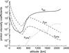 |
Fig. 8 Dynamic viscosity coefficients (6), (8–10) without the magnetic field for protons in the lower solar atmosphere. Here ηpp is plotted in units 10-8 kg/(s m) and all other coefficients in 10-10 kg/m3. |
The coefficient μpp is not presented because from the second row in Eq. (4) it is seen that for a = b its contribution vanishes. Therefore the most dominant μab terms should be checked only for the case a ≠ b. From Fig. 8 it is clear that in most of the space the coefficient μpH should be taken into account. However, above an altitude of about 1700 km the viscosity between protons and helium ions becomes the most dominant, as is seen from the dotted line, which gives the values of μpHe+, though this may change if protons are magnetized; then the gyro-viscosity should be taken into account. This problem will be discussed elsewhere. Furthermore the viscosity that involves neutral helium μpHe is clearly negligible everywhere.
It is meaningless to directly compare the leading μab term with ηpp because they are in different units. Instead, one must compare the complete corresponding viscosity terms from the first and second row in Eq. (4), which is approximately  (11)For waves with the wave number k we have Lv ≃ 1/k. Because the ratio ηpp/μpH changes with altitude for many orders of the magnitude, the relative contribution of the two terms to the viscosity will drastically change. For example, at x = 0 we have ηpp/μpH = 0.22 [m2/s] and at x = 1580 km ηpp/μpH = 3.2 × 10⁴ [m2/s]. The speed difference δvi may be time dependent, for instance for waves that first affect some charged species a while the un-charged species b is set into motion only after some collisional time, which will also affect the ratio (11).
Without relative motion between protons and other species, the proton viscosity is strictly self-induced. With relative motion the situation becomes much more complicated and it is not so obvious which terms are more dominant. This is true in particular in view of ratio (16), which involves friction (see below). Hence, to be on a safe ground, one should keep the two leading viscosity terms discussed above together with the corresponding friction force terms.
A similar analysis is now used for the conductivity vector (5). For unperturbed situations the second row in Eq. (5) can usually be neglected because i) collisions couple separate species and they are expected to move together; and ii) in the presence of frequent collisions thermalization is very effective, so the temperatures are equal. This does not necessarily hold for some accidental electrostatic or electromagnetic perturbations. For example, electrostatic ion-acoustic-type perturbations in the given environment must involve ion temperature perturbations (because the wave phase speed is on the same order as the ion thermal speed), and this happens on the background of initially static neutrals. Therefore the second row in (5) should be kept. For protons, keeping the most relevant terms as above, we have the x-component of the conductivity vector ![Mathematical equation: \begin{eqnarray*} Q_{{\rm p}x}&=&-\kappa_{\rm pp} \frac{\partial}{\partial x}\left(\kappa T\right) + \chi_{\rm p\sss{\rm H}} \left(v_{\sss{\rm H},x}-v_{{\rm p},x}\right) \left[\!\left(\vec v_{\sss{\rm H}}-\vec v_{\rm p}\right)^2\!- \!5 \frac{\kappa \left(\!T_{\sss{\rm H}}\! - \!T_{\rm p}\!\right)}{m_{\sss{\rm H}}\! + \!m_{\rm p}}\!\right] \\ &&\quad + \chi_{\rm p\sss{\rm H}e}\left(v_{\rm \sss{\rm H}e,x}-v_{{\rm p},x}\right)\left[ \left(\vec v_{\rm \sss{\rm H}e}-\vec v_{\rm p}\right)^2 -5 \frac{\kappa \left(T_{\rm \sss{\rm H}e} - T_{\rm p}\right)}{m_{\rm \sss{\rm H}e} + m_{\rm p}}\right] \\ &&\quad + \chi_{\rm p\sss{\rm H}e^+}\left(v_{\rm \sss{\rm H}e^+,x}-v_{{\rm p},x}\right)\left[ \left(\vec v_{\rm \sss{\rm H}e^+}-\vec v_{\rm p}\right)^2 -5 \frac{\kappa \left(T_{\rm \sss{\rm H}e^+} - T_{\rm p}\right)}{m_{\rm \sss{\rm H}e^+} + m_{\rm p}}\right]\cdot \end{eqnarray*}](/articles/aa/full_html/2013/06/aa20738-12/aa20738-12-eq132.png) In view of Eq. (5), the thermal conductivity coefficients which appear here are
In view of Eq. (5), the thermal conductivity coefficients which appear here are ![Mathematical equation: \begin{eqnarray} &&\kappa_{\rm pp}=\frac{5}{3} \frac{n_{\rm p} v_{\rm {\sss T}p}^2}{\nu_{\rm pp}+ \nu_{\rm p{\sss {\rm H}}} + \nu_{\rm p{\sss {\rm H}}e} + \nu_{\rm p{\sss {\rm H}}e^+}}, \quad \left[\frac{1}{\rm s\, m}\right], \label{kpp} \\ && \chi_{\rm p\sss{\rm H}}=\frac{1}{3}\frac{m_{\rm p} n_{\rm p} \nu_{\rm p{\sss {\rm H}}}}{\nu_{\rm pp}+ \nu_{\rm p{\sss {\rm H}}} + \nu_{\rm p{\sss {\rm H}}e} + \nu_{\rm p{\sss {\rm H}}e^+}}, \quad \left[\frac{\rm kg}{\rm m^3}\right], \label{kajh} \\ &&\chi_{\rm p\sss{\rm H}e}=\frac{1}{3}\frac{m_{\rm p} n_{\rm p} \nu_{\rm p{\sss {\rm H}}e}}{\nu_{\rm pp}+ \nu_{\rm p{\sss {\rm H}}} + \nu_{\rm p{\sss {\rm H}}e} + \nu_{\rm p{\sss {\rm H}}e^+}}, \label{kajhe} \\ &&\chi_{\rm p\sss{\rm H}e^+}=\frac{1}{3}\frac{m_{\rm p} n_{\rm p} \nu_{\rm p{\sss {\rm H}}e^+}}{\nu_{\rm pp}+ \nu_{\rm p{\sss {\rm H}}} + \nu_{\rm p{\sss {\rm H}}e} + \nu_{\rm p{\sss {\rm H}}e^+}}\cdot\label{kajhei} \end{eqnarray}](/articles/aa/full_html/2013/06/aa20738-12/aa20738-12-eq133.png) Here, similar to Eqs. (6)–(10), all parameters are altitude dependent, which affects the thermal conductivity coefficients (12−15), whose altitude dependence is presented in Fig. 9 in units 1020 (s m)-1 for κpp, and 10-10 kg/m3 for χpb coefficients. Similar to viscosity, regarding χpb coefficients, here again proton interaction with hydrogen atoms is most dominant below 1700 km and only χpH should be kept in the part that describes the interaction between different species in Eq. (5). Above this altitude one should keep χpHe+ only. These conclusions hold as long as the ions are unmagnetized (gyro-viscosity excluded). Identifying these most dominant terms can significantly simplify the derivations.
Here, similar to Eqs. (6)–(10), all parameters are altitude dependent, which affects the thermal conductivity coefficients (12−15), whose altitude dependence is presented in Fig. 9 in units 1020 (s m)-1 for κpp, and 10-10 kg/m3 for χpb coefficients. Similar to viscosity, regarding χpb coefficients, here again proton interaction with hydrogen atoms is most dominant below 1700 km and only χpH should be kept in the part that describes the interaction between different species in Eq. (5). Above this altitude one should keep χpHe+ only. These conclusions hold as long as the ions are unmagnetized (gyro-viscosity excluded). Identifying these most dominant terms can significantly simplify the derivations.
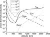 |
Fig. 9 Proton thermal conductivity coefficients (12–15) with altitude; κpp is plotted in (s m)-1, and χpj in kg/m3. |
6.2. Friction vs. viscosity. Vanishing friction
Comparing the contribution to the momentum equation of the viscosity term from the second row in Eq. (4) and the usual friction force yields the following approximate dimensionless ratio of these terms for the species a: 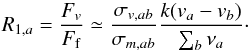 (16)Here, we estimate the interaction between the species a and another single species b, and σv,ab/σm,ab < 1 is the ratio of the cross sections for viscosity and momentum transfer (which are typically different, see Figs. 1–3), and k-1 ≡ λ is the characteristic scale length for the speed difference (e.g., wave length for wave analysis), which appears from ∇·Πa,ij in the momentum equation. It is clear that R1,a can have any value (e.g., because the difference va − vb may be time dependent for electromagnetic or electrostatic wave phenomena that affect the charged species a first). Therefore it cannot be justified to neglect the second row in Eq. (4) in the wave analysis. Assuming that a represents charged species and b some neutral one, for electromagnetic or electrostatic perturbations species b is initially at rest so that R1,a < 1 if
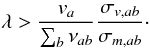 For these wavelengths the contribution of the second row in the viscosity in Eq. (4) is negligible, but this holds in principle for the initial regime only.
Comparing now the viscosity contribution to the momentum equation due to the first row in Eq. (4), with the friction force between a and b for the initial stage with vb = 0, yields 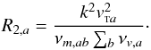 (17)The friction force dominates if
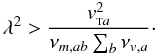 The index m here denotes the collision frequency calculated with the appropriate cross section for momentum transfer. Hence, the friction force is stronger provided that the wavelength exceeds both of these expressions, i.e.,
  (18)The presented conclusions hold for the initial regime only. The species are coupled through collisions and the speed difference va − vb, in both the friction force and in the viscosity terms containing the speed difference may approach zero provided the time interval is long enough. This issue (related to friction force) has been discussed in Vranjes et al. (2008a). The velocity difference relaxation is altitude dependent, and after presenting the detailed collision frequencies in the previous sections, we can make some estimates for proton interaction with neutrals. Assuming that protons start to move with some initial speed vp0 through static background of hydrogen atoms, we can calculate the time needed for both species to achieve some common speed vc, which naturally must be between 0 and vp0. This is performed for several layers to see the differences caused by density and temperature variation. Starting from the momentum equations with friction only ∂vn/∂t = νnp(vp − vn), ∂vp/∂t = νpn(vn − vp), we find the time dependent velocity of the two species:
 ![Mathematical equation: \begin{eqnarray} && \vec v_{\rm n}=v_{\rm c} + \frac{\left(\vec v_{\rm n0} - \vec v_{\rm p0}\right) \nu_{\rm np}}{\nu_{\rm pn}+ \nu_{\rm np}} \exp[-(\nu_{\rm pn} + \nu_{\rm np})t], \label{pari} \\ &&\vec v_{\rm p}=v_{\rm c} - \frac{\left(\vec v_{\rm n0} -\vec v_{\rm p0}\right) \nu_{\rm pn}}{\nu_{\rm pn}+ \nu_{\rm np}} \exp[-(\nu_{\rm pn} + \nu_{\rm np})t]. \label{parn} \end{eqnarray}](/articles/aa/full_html/2013/06/aa20738-12/aa20738-12-eq159.png) Taking mp ~ mn and vn0 = 0, we obtain for the common velocity for both species
Taking mp ~ mn and vn0 = 0, we obtain for the common velocity for both species  (21)
(21)
Common velocity and velocity relaxation time tc for protons (with arbitrary starting speed vp0) and hydrogen (with vn0 = 0) for several altitudes.
In Table 1 the common speed (21) is given for several altitudes, and the time necessary for both species to achieve 99 percent of this common speed is calculated from
![Mathematical equation: $$ t_{\rm c}=-\frac{\ln[0.01]}{\nu_{\rm pn} \left(1+ n_{\rm p}/n_{\rm n}\right)} \cdot $$](/articles/aa/full_html/2013/06/aa20738-12/aa20738-12-eq176.png) To calculate νpn, which appears here, we used the cross section for momentum transfer from Fig. 1.
To calculate νpn, which appears here, we used the cross section for momentum transfer from Fig. 1.
From Table 1 we can conclude the following. a) Because of the very frequent collisions between the two species, the friction between them should vanish very quickly, but b) at the same time this must have a strong effect on the small electrostatic or electromagnetic perturbations that are now supposed to set into motion the two species. This implies c) that the amplitude of these perturbations must reduce dramatically. d) Because the two species move together (after the collisional time tc), the friction is effectively zero, therefore the only relevant remaining dissipation mechanism must be through viscosity. e) All these conclusions are altitude dependent; higher up the friction may become dominant dissipation process, in particular for a certain wavelength regime, as predicted by Eq. (18).
These facts are frequently overlooked in the literature where such a regime of common motion is just assumed [but without much regard to the consequence c) above] and equations for different components are summed up, and a single fluid dynamics is then studied. This implies that the transition process, that takes place within the collision time, is neglected together with the physical phenomena involved in the process. This problem is discussed in Vranjes et al. (2008a). A statement of the validity of common equations for all species is given also in Alfvén & Fälthammar (1963 on p. 177), where the authors write that the common speed has sense only if the speed of neutrals is nearly equal to the speed of plasma. Such a situation surely cannot be expected in the initial stadium of some electrostatic or electromagnetic perturbations that naturally affect plasma species first, with the background of initially immobile neutrals whose dynamics develops due to friction and partly due to viscosity, and this after the collisional time only (Vranjes et al. 2008a). In the present work we are able to quantify these phenomena by calculating the precise characteristic collisional time and consequently by predicting the amplitude of the common speed achieved within such a time interval.
6.3. Hydrogen dynamics
We have seen that proton interaction with neutral hydrogen is the most dominant in most of the space, so in a proper wave analysis that obeys conservation laws, one needs the continuity, momentum, and energy equations describing hydrogen dynamics as well. Hydrogen collision frequencies with other species (electrons, ions, and helium atoms) and corresponding cross sections can easily be obtained using the momentum conservation  (22)For completeness, the collision frequency νHp for the most dominant neutral hydrogen atom collisions with protons is presented in Fig. 10 for the elastic scattering (dashed line) and momentum transfer (dotted line). The local minimum in the profile is due to the decrease in the profile of target particles (protons).
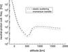 |
Fig. 10 Collision frequency for H − p collisions. |
We furthermore need components for hydrogen viscosity and thermal conductivity. For ηHH,κHH we may set 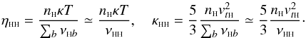 (23)With the cross section σHH determined by line 2 in Fig. 3, the dynamic viscosity coefficient for hydrogen self-collisions becomes
 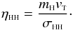 (24)In writing it we used νHH = σHHnHvT.
In the literature one can find also the expression that follows from the Chapman & Cowling (1953) model based on the interaction of hard spheres: 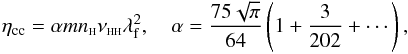 (25)where
  is the mean free path, and rH is the diameter of the colliding particles, in the present case its value is rH = 2.12 × 10⁻¹⁰ m. This yields
 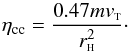 (26)The expressions (24) and (26) are checked against experimental measurements available in Vargaftik et al. (1996) for a hydrogen gas, and the results for several temperatures are presented in Table 2. In the given energy range our ηHH gives values closer to the experimental ones. The differences between the two models are about factor 2, which is clearly due to indistinguishability effect that is missing in the Chapman and Cowling classical model.
Hydrogen dynamic viscosity coefficient [in units kg/(s m) = Pa s] for several temperatures.
Using the Chapman & Cowling (1953) model, we can also calculate the coefficient of thermal conductivity for hydrogen gas ![Mathematical equation: \begin{eqnarray} \kappa_{\rm cc}&=&n_{{\sss {\rm H}}} \frac{5 \sqrt{\pi}}{16} \left(1+ \frac{1}{44}+\cdots\right) \nu_{{\rm \sss HH}} \lambda_{\rm f}^2\simeq \frac{5}{16\sqrt{2 \pi}} \left(1+ \frac{1}{44}\right)\frac{ v_{{\rm \sss T}}}{r_{{\sss {\rm H}}}^2}\nonumber \\ &=&2.84\times 10^{18} v_{{\rm \sss T}}, \quad \mbox{[in } \rm (s\,m)^{-1}]. \label{ve4} \end{eqnarray}](/articles/aa/full_html/2013/06/aa20738-12/aa20738-12-eq214.png) (27)This can be compared with the above-given corresponding coefficient (23) obtained from kinetic theory with the BGK collision integral:
(27)This can be compared with the above-given corresponding coefficient (23) obtained from kinetic theory with the BGK collision integral: 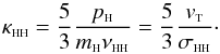 (28)Around the temperature minimum region in the photosphere, using line 2 from Fig. 3 for hydrogen, our conductivity coefficient κHH is higher by about a factor 2 than the Chapman and Cowling coefficient (27), which is the consequence of the quantum-mechanical indistinguishability incorporated in our derivations.
For the viscosity coefficients μHb, which are associated with the terms containing the speed difference between H and b species, the situation is as follows: The speed difference between different neutral species cannot be of any importance for obvious reasons (they are coupled through collisions, they react similarly to perturbations by external forces). Hence, both μHH and μHHe are not needed for the same reason. We now compare 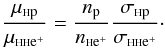 From Fontenla et al. (1993) we know that np ≫ nHe+ in the whole region of interest here. Therefore μHHe+ is most likely negligible. Using (22) we have
 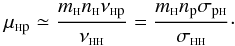 (29)Similar arguments are used for the coefficients χHb in the conductivity vector. Hence, the only remaining coefficient we need is
 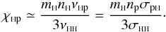 (30)The most important coefficients for hydrogen ηHH, μHp, κHH, χHp are presented in Fig. 11. Evidently, for practical purposes in the lower solar atmosphere the self-interaction coefficients ηHH,κHH may be taken as constant and their values are ≃0.5 × 10⁻⁴ kg/(sm) and ≃5 × 10²³ (sm)-1, respectively. The other two coefficients μHp and χHp, which include interaction with other species are strongly altitude dependent.
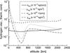 |
Fig. 11 Most relevant viscosity (ηHH,μHp) and thermal conductivity (κHH,χHp) coefficients for hydrogen atoms. |
7. Summary and discussions
The parameters in the lower solar atmosphere change with altitude and much care is needed to properly describe the physical processes that take place there. One obvious example is presented in Fig. 5 where the e-H collision frequency changes by seven orders of magnitude between the altitudes of −100 km and 2200 km, taking values 1.3 × 10¹⁰ Hz and 2.4 × 10³ Hz, respectively. In addition to this, the type of collisions changes as well, e-H collisions being the most dominant up to 900 km and e-p collisions above that. A detailed knowledge of these processes is essential to estimate the friction and related phenomena (e.g. conductivity, transport, etc.).
Our most important conclusions can be summarized as follows:
-
The cross sections presented in Sect. 2.1 are themost accurate existing ones. They contain the following essentialdetails: a) variation of cross sections with temperature (altitude);b) variation of cross sections due to quantum effects in the givenlow-temperature range in the lower solar atmosphere; and c) clearand pronounced differences of cross sections describing elasticscattering, momentum transfer, and viscosity. Combined, thesefine details may introduce significant differences for variousprocesses related to magnetization, transport, heating, etc. Al-though well-known in the laboratory plasmas, so far these detailshave not been studied in the solar atmosphere. Unlike the variousapproximate data, the data we used here (all of them from citedreferences) are fully quantum-mechanical and obtained without(almost) any approximation, thus are the most accurate data everobtained in collisional physics (numerical accuracy to six sig-nificant digits, physical accuracy bellow one percent). The onlyassumption used in their derivation was that the electronic exci-tation to the excited nonresonant electronic states is negligible(though charge transfer is included). This approximation is quiteaccurate below the energy threshold for electronic excitation andthis is the source of the physical accuracy of “only” one percent. Inderiving these data even ro-vibrational degrees of freedom weretaken, and they are created to serve as a benchmark for checkingthe accuracy of other approximate approaches. Needless to say,we used the exact ion-atom potentials from R = 0 to R = 80 000 a.u. The cross sections presented here, coincide with classical at high energies. At low energies (roughly below 1 eV) the cross sections include the effects of a) indistinguishability and b) charge transfer. The lower solar atmosphere is indeed within this low-energy range, and consequently these intrinsic properties of the plasma-gas matter cannot be avoided. The accuracy of our collision data for ion-atom collisions removes possible doubts on the size of the momentum exchange used in previous works available in the literature, including possible under- or overestimation of the role of Alfvén waves and kink wave damping in the lower solar atmosphere.
-
ii)
For electron dynamics above 850 km neutrals plays no practical role, although the neutral number density at 850 km is still three orders of magnitude higher than that of protons and electrons. However, this may not be so if inelastic collisions are taken into account, e.g., those in which electrons are lost or created, as discussed in Sect. 2. These phenomena are beyond the scope of the present work.
-
iii)
For proton dynamics the role of neutrals is negligible above 1900 km, although at this altitude (according to data from Fontenla et al. 1993) np = 4.24 × 10¹⁶ m-3 is still below the neutral hydrogen density nH = 1.7 × 10¹⁷ m-3. We stress again that this conclusion may not hold if inelastic collisions are taken into account.
-
iv)
There exists a layer within which both electrons and ions are definitely unmagnetized. For intense magnetic structures with a magnetic field of 0.1 T this layer is located around an altitude x = 0 and below. In this layer the magnetic field plays no direct role in the dynamics of both electrons and ions.
-
v)
The layer of unmagnetized electrons and ions continues with a much thicker layer in which electrons are magnetized and ions are not. The depth of this layer changes spatially, and for protons it is at least 1000 km thick in regions with a kilo-Gauss magnetic field. The dynamics of electrons and ions in this region is completely different, and models that assume a two-component system consisting of “neutrals” on one side and “plasma” on the other are meaningless. This is because the “plasma” contains electrons and ions whose dynamics is totally different because of the magnetic field. Consequently, in this layer the electrons and ions cannot be treated as a single fluid. A fully multi-component analysis (fluid or kinetic) has no alternative in the lower solar atmosphere.
-
vi)
Viscosity and thermal conductivity coefficients given in this work are currently the most accurate, and at the same time the most complete ones because they contain all most relevant terms appropriate for a multi-component system such as is the lower solar atmosphere with unmagnetized ions. They also completely agree with experimental measurements. Our results show that including viscosity both for protons and neutral hydrogen may be essential to properly capture diffusion phenomena in the solar atmosphere.
If we return back to Fig. 1, we see that the proton-hydrogen cross section changes with temperature (i.e. with the altitude). Its values for elastic scattering (in the laboratory frame) are 2.269 × 10⁻¹⁸ m2 and 1.601 × 10⁻¹⁸ m2 at temperatures of 5 × 10³ K and 20 × 103 K, respectively. The temperature of 5 × 10³ K corresponds to the altitude 200 km (and also 705 km), and 20 × 103 K corresponds to the altitude ≃2200 km. We can can now compare these with the cross section used by other researchers, e.g., Zaqarashvili et al. (2011b), where the cross section was assumed to be constant with the value 8.79 × 10⁻²¹ m2, i.e., π a.u., describing collisions where ions and neutrals are treated as hard spheres. Our correct values, which include the quantum-mechanical effect of indistinguishability, for the two temperatures given above are 258 and 182 times greater! We note that these authors make no distinction between cross sections for elastic scattering and momentum transfer. Therefore we can also compare their value with our cross section for the momentum transfer from the same figure; for the two temperatures we have 1.040 × 10⁻¹⁸ m2 and 8.785 × 10⁻¹⁹ m-2. These are again 118 and 100 times greater than their values. We observe that in the mentioned work the proton-helium cross section is assumed to be the same as the one for proton-hydrogen collisions given above. However, from our Fig. 2 the cross sections for p-He elastic scattering at 5 × 10³ K and 20 × 103 K in the laboratory frame are about 110 and 70 times greater than their value. At the same time, our cross section for momentum transfer for the two temperatures is 20 and 8 times greater than their value.
On the other hand, the cross section for p-H collisions in Khomenko & Collados (2012) is fixed to 5 × 10-19 m2, which is rather close to our value for the momentum transfer cross section in plasma reference frame, roughly speaking only twice as smaller. Though in their subsequent calculation of the collision frequency this difference is compensated by the numerical factor 81/2, which they keep in the thermal velocity, and the collision frequency which they obtain is very close to our value.
In view of the results presented here a natural next step is to include effects of inelastic collisions. In our previous work (Vranjes & Poedts 2006b) we have shown that in certain layers in the photosphere all ions in a unit volume recombine at least 26 times per second. This may have consequences on magnetization, for example. Perhaps this may be used also to explain the nature and longevity of prominences, which are believed to
contain considerable amounts of neutrals. Their longevity is a challenge for the theory because neutrals should naturally diffuse and evacuate a prominence by moving to lower layers due to gravity. However, in the presence of inelastic collisions this diffusion should take place at reduced speed because a neutral particle does not remain neutral all the time, it is consequently affected by the magnetic field and the prominence may last longer.
References
- Alfvén, H., & Fälthammar, C. G. 1963, Cosmical Electrodynamics (Oxford: Clarendon Press), 177 [Google Scholar]
- Arber, T. D., Haynes, M., & Leake, J. E., ApJ, 666, 541 [Google Scholar]
- Barceló, S., Carbonell, M., & Ballester, J. L. 2011, A&A, 525, A60 [NASA ADS] [CrossRef] [EDP Sciences] [Google Scholar]
- Bates, D. R. 1951, Proc. Phys. Soc. B, 64, 805 [Google Scholar]
- Bedersen, B., & Kieffer, L. J. 1971, Rev. Mod. Phys., 43, 601 [NASA ADS] [CrossRef] [Google Scholar]
- Brackmann, R. T., Fite, W. L., & Neynaber, R. H. 1958, Phys. Rev., 112, 1157 [NASA ADS] [CrossRef] [Google Scholar]
- Brode, R. B. 1933, Rev. Mod. Phys., 5, 257 [NASA ADS] [CrossRef] [Google Scholar]
- Brandsen, B. H. 1970, Atomic Collision Theory (New York: Benjamin) [Google Scholar]
- Chapman, S., & Cowling, T. G. 1953, The Mathematical Theory of Nonuniform Gasses (Cambridge: Cambridge Univ. Press) [Google Scholar]
- Chen, F. F., & Chang, J. P. 2003, Lect. Notes on Principles of Plasma Processing (New York: Kluwer Academic/Plenum Publishers) [Google Scholar]
- Dalgarno, A. 1961, Proc. R. Soc. Lond. A, 252, 132 [NASA ADS] [Google Scholar]
- Dalgarno, A., McDowell, M. R. C., & Williams, A. 1958, Phil. Trans. R. Soc. Lond. A, 250, 411 [NASA ADS] [CrossRef] [Google Scholar]
- Fortov, V. E., Iakubov, I. A., & Khrapak, A. G. 2006, Physics of Strongly Coupled Plasma (Oxford: Clarendon Press) [Google Scholar]
- Fontenla, J. M., Avrett, E. H., & Loeser, R. 1993, ApJ, 406, 319 [NASA ADS] [CrossRef] [Google Scholar]
- Ratcliffe, J. A. 1959, The Magneto-Ionic Theory and its Applications to the Ionosphere (Cambridge: Cambridge Univ. Press) 33 [Google Scholar]
- Glassgold, A. E., Krstic, P. S., & Schultz, D. R. 2005, ApJ, 621, 808 [NASA ADS] [CrossRef] [Google Scholar]
- Hasted, J. B. 1964, Physics of Atomic Collision (London: Butterworths) [Google Scholar]
- Jaeggli, S. A., Lin, H., & Uitenbroek, H. 2012, ApJ, 745, 133 [NASA ADS] [CrossRef] [Google Scholar]
- Jamieson, M. J., Dalgarno, A., Zygelman, B., Krstic, P. S., & Schultz, D. R. 2000, Phys. Rev. A, 61, 14701 [NASA ADS] [CrossRef] [Google Scholar]
- Khomenko, E., & Collados, M. 2012, ApJ, 747, 87 [NASA ADS] [CrossRef] [Google Scholar]
- Khomenko, E., Centeno, R., Collados, M., & Trujillo Bueno, J. 2008, ApJ, 676, L85 [NASA ADS] [CrossRef] [Google Scholar]
- Kieffer, L. J. 1971, Atomic Data, 2, 293 [NASA ADS] [CrossRef] [Google Scholar]
- Krstic, P. S., & Schultz, D. R. 1998, Atomic and Plasma-Material Interaction Data for Fusion, IAEA, Vienna, 8 [Google Scholar]
- Krstic, P. S., & Schultz, D. R. 1999a, J. Phys. B: At. Mol. Opt. Phys., 32, 3485 [NASA ADS] [CrossRef] [Google Scholar]
- Krstic, P. S., & Schultz, D. R. 1999b, Phys. Rev. A, 60, 2118 [CrossRef] [Google Scholar]
- Makabe, T., & Petrovic, Z. 2006, Plasma Electronics (Boca Raton: Taylor & Francis) [Google Scholar]
- McDowell, M. R. C., & Coleman, J. P. 1970, Introduction to the Theory of Ion-Atom Collisions (Amsterdam: North-Holland Pub. Co.) [Google Scholar]
- Mitchner, M., & Kruger, C. H. 1973, Partially Ionized Gases (New York: John Wiley Sons), 102 [Google Scholar]
- Pandey, B. P., & Wardle, M. 2008, MNRAS, 385, 2269 [NASA ADS] [CrossRef] [Google Scholar]
- Purcell, E. M., & Field, G. B. 1956, ApJ, 124, 542 [NASA ADS] [CrossRef] [Google Scholar]
- Schultz, D. R., Krstic, P. S., Lee, T. G., & Raymond, J. C. 2008, ApJ, 678, 950 [NASA ADS] [CrossRef] [Google Scholar]
- Schunk, R. W., & Nagy, A. F. 2009, Ionospheres: Physics, Plasma Physics, and Chemistry (Cambridge: Cambridge Univ. Press) [Google Scholar]
- Soler, R., Oliver, R., & Ballester, J. L. A&A, 512, A28 [Google Scholar]
- Spitzer, L. 1962, Physics of fully ionized gasses (New York, London: Intersience Publishers), 146 [Google Scholar]
- Tawara, H., Itikawa, Y., Nishimura, H., & Yoshino, M. 1990, J. Phys. Chem. Ref. Data, 19, 617 [Google Scholar]
- Vargaftik, N., Vinogradov, Y. K., & Yargin, V. S. 1996, Handbook of Physical Properties of Liquids and Gasses (New York: Begell House) [Google Scholar]
- Vranjes, J., & Poedts, S. 2006a, A&A, 458, 635 [NASA ADS] [CrossRef] [EDP Sciences] [Google Scholar]
- Vranjes, J., & Poedts, S. 2006b, Phys. Lett. A, 348, 346 [NASA ADS] [CrossRef] [Google Scholar]
- Vranjes, J., & Poedts, S. 2008, Phys. Plasmas, 15, 034504 [NASA ADS] [CrossRef] [Google Scholar]
- Vranjes, J., Tanaka, M. Y., Pandey, B. P., & Kono, M. 2002, Phys. Rev. E., 66, 037401 [NASA ADS] [CrossRef] [Google Scholar]
- Vranjes, J., Poedts, S., & Pandey, B. P. 2007, Phys. Rev. Lett., 98, 049501 [NASA ADS] [CrossRef] [Google Scholar]
- Vranjes, J., Poedts, S, Pandey, B. P., & De Pontieu, B. 2008a, A&A, 478, 553 [NASA ADS] [CrossRef] [EDP Sciences] [Google Scholar]
- Vranjes, J., Kono, M., Poedts, S., & Tanaka, M. Y. 2008b, Phys. Plasmas, 15, 092107 [NASA ADS] [CrossRef] [Google Scholar]
- Zaqarashvili, T. V., Khodachenko, M. L., & Rucker, H. O. 2011a, A&A, 529, A82 [NASA ADS] [CrossRef] [EDP Sciences] [Google Scholar]
- Zaqarashvili, T. V., Khodachenko, M. L., & Rucker, H. O. 2011b, A&A, 534, A93 [NASA ADS] [CrossRef] [EDP Sciences] [Google Scholar]
All Tables
Common velocity and velocity relaxation time tc for protons (with arbitrary starting speed vp0) and hydrogen (with vn0 = 0) for several altitudes.
Hydrogen dynamic viscosity coefficient [in units kg/(s m) = Pa s] for several temperatures.
All Figures
|
Fig. 1 Integral cross sections σpH for proton (p) collisions with neutral hydrogen atoms H for quantum-mechanically indistinguishable nuclei of the projectile and target particles, following Krstic & Schultz (1998). Here and throughout the text 1 a.u. = 2.8 × 10⁻²¹ m2, 1 eV ≃ 11 604 K. |
| In the text | |
|
Fig. 2 Integral cross sections σpHe for proton collisions with neutral helium He. |
| In the text | |
|
Fig. 3 Integral cross section σHH for collisions between neutral hydrogen atoms H for quantum-mechanically indistinguishable nuclei. |
| In the text | |
|
Fig. 4 Cross section for elastic scattering of electrons on neutral hydrogen atoms H and neutral helium atoms He, in terms of the electron energy. |
| In the text | |
|
Fig. 5 Electron collisions with the altitude. For comparison, the thin line gives the electron gyro-frequency Ωe for the starting value of the magnetic field B0 = 0.1 T. |
| In the text | |
|
Fig. 6 Coulomb collisions of protons in terms of altitude. |
| In the text | |
|
Fig. 7 Collision frequency for protons colliding with the neutral atoms H and He. |
| In the text | |
|
Fig. 8 Dynamic viscosity coefficients (6), (8–10) without the magnetic field for protons in the lower solar atmosphere. Here ηpp is plotted in units 10-8 kg/(s m) and all other coefficients in 10-10 kg/m3. |
| In the text | |
|
Fig. 9 Proton thermal conductivity coefficients (12–15) with altitude; κpp is plotted in (s m)-1, and χpj in kg/m3. |
| In the text | |
|
Fig. 10 Collision frequency for H − p collisions. |
| In the text | |
|
Fig. 11 Most relevant viscosity (ηHH,μHp) and thermal conductivity (κHH,χHp) coefficients for hydrogen atoms. |
| In the text | |
Current usage metrics show cumulative count of Article Views (full-text article views including HTML views, PDF and ePub downloads, according to the available data) and Abstracts Views on Vision4Press platform.
Data correspond to usage on the plateform after 2015. The current usage metrics is available 48-96 hours after online publication and is updated daily on week days.
Initial download of the metrics may take a while.