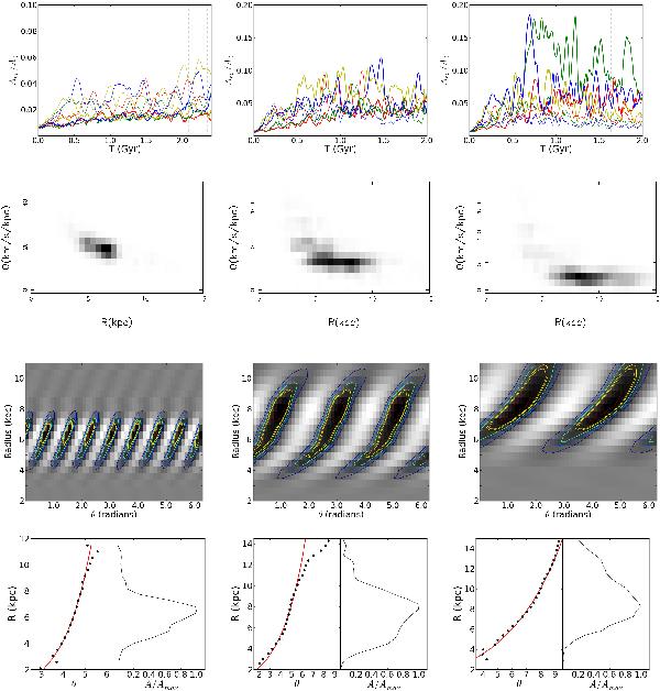
Top row: amplitudes calculated from Eq. (10) and averaged over a radial range of 4−10 kpc of spiral modes m = 1 (thick red); 2 (thick green); 3 (thick blue); 4 (thick yellow); 5 (thin red); 6 (thin green); 7 (thin blue), and 8 (thin yellow) normalised to the axisymmetric m = 0 mode, as a function of time for simulations R (left), F (middle), and K (right). Vertical dashed lines represent the time window of a Fourier transform applied in Sect. 3.1. Second row: power spectra calculated from Eq. (12) of simulation R for the m = 8 mode (left), F for the m = 3 mode (middle), and K for the m = 2 mode (right). Prominent ridges (dark pixels) span between 4−10 kpc in most cases. Third row: in polar coordinates, the density map of the dominant density wave mode pattern selected from rows of , 30, and 24 km s^-1 kpc^-1 for simulations R, F, and K respectively. White regions indicate areas of low density and black regions indicate areas of high density. Contours emphasis the highest density regions. Bottom panels: dominant mode pattern positions (black points) calculated from Eq. (13) in the azimuth-radius plane for the corresponding patterns in the row above. The red lines show the lines of best fit for each pattern. The right side of each panel shows the radial amplitude profile, which is used to weight the fitting.