| Issue |
A&A
Volume 552, April 2013
|
|
|---|---|---|
| Article Number | A41 | |
| Number of page(s) | 7 | |
| Section | Astronomical instrumentation | |
| DOI | https://doi.org/10.1051/0004-6361/201321092 | |
| Published online | 20 March 2013 | |
A Fourier domain model for estimating astrometry errors due to static and quasi-static optical surface errors
TMT Observatory CorporationInstrumentation Department,
1111 S. Arroyo Pkwy. Ste. 200,
Pasadena,
CA,
91107
USA
e-mail: This email address is being protected from spambots. You need JavaScript enabled to view it.
Received:
12
January
2013
Accepted:
25
February
2013
Abstract
Context. The wavefront aberrations due to optical surface errors in adaptive optics systems and science instruments can be a significant error source for high precision astrometry.
Aims. This report derives formulas for evaluating these errors which may be useful in developing astrometry error budgets and optical surface quality specifications.
Methods. A Fourier domain approach is used, and the errors on each optical surface are modeled as “phase screens” with stationary statistics at one or several conjugate ranges from the optical system pupil. Three classes of error are considered: (i) errors in initially calibrating the effects of static surface errors; (ii) the effects of beam translation, or “wander,” across optical surfaces due to (for example) instrument boresighting error; and (iii) quasistatic surface errors which change from one observation to the next.
Results. For each of these effects, we develop formulas describing the position estimation errors in a single observation of a science field, as well as the differential error between two separate observations. Sample numerical results are presented for the three classes of error, including some sample computations for the Thirty Meter Telescope and the NFIRAOS first-light adaptive optics system.
Key words: astrometry / instrumentation: high angular resolution / instrumentation: adaptive optics
© ESO, 2013
1. Introduction
High precision astrometry is becoming an increasingly important capability for large, and future extremely large, optical and near-infra-red astronomical telescopes (Yelda et al. 2010; Fritz et al. 2010; Trippe et al. 2010). Astrometric accuracies of 40 to 100 micro arc seconds (μas) have now been reported for observations both without and with adaptive optics (Lazorenko et al. 2009; Cameron et al. 2009), and requirements for future systems are specified in the 10 to 50 μas range (TMT Science Requirements Document, at http://www.tmt.org/documents). Much as for high contrast imaging, performance at this level will require the careful evaluation of the full range of possible error sources, some of which have been considered negligible up to now. One sample astrometry error budget includes at least 35 different terms, grouped into the five categories of: reference star catalog errors, atmospheric refraction effects, atmospherc turbulence effects, focal plane measurement errors, and opto-mechanical errors (Schoeck 2011). This final category places challenging requirements on the design, fabrication, and alignment of science instruments (and adaptive optical systems) in order to control this systematic error source.
The purpose of this paper is to describe a set of engineering formulas for estimating the astrometry errors due to surface errors in opto-mechanical systems. These formulas can be used to develop quantitative error budgets and the corresponding optical surface specifications. A Fourier domain approach is used, and the phase errors on each optical surface are modeled as “phase screens” with shift-invariant statistics at one or several conjugate ranges from the optical system pupil. The image distortion errors inherit this property of stationarity, and some steps of the work consequently resemble previous analysis of tilt anisoplanatism in adaptive optical (AO) systems (Roddier et al. 1993). The errors are evaluated as weighted integrals of the power spectral densities (PSDs) of the errors on each optical surface, where the values of the weighting functions depend upon parameters including the telescope aperture diameter, science field-of-view (FoV) diameter, conjugate range to the optical surface, and the category of optical surface effect evaluated.
Section 2 formulates a model for the three different types of optical surface effects considered in the analysis. These are:
-
the static calibration undersampling error from using only a finite number of reference sources to sample the image distortion pattern in the focal plane;
-
the error due to random or systematic beam wander translation across the static errors on each surface, which could occur due to an instrument boresighting error or image derotation; and
-
quasi-static errors due to time-varying optical surface errors, for example a calibration error on a deformable mirror in a multi-conjugate AO (MCAO) system.
We develop a notation to keep track of these various errors, both for a single observation of a science field and the differential error between two successive observations. We formulate a model for on-sky calibration of the errors (using known reference stars in the image) in terms of removing the low-order modes of the image distortion pattern, such as global tip/tilt and plate scale.
The analytical methods used to evaluate these errors are developed in Sects. 3 through 5. Section 3 describes our standard geometrical optics model for the image distortion due to a set of optical surface errors. Section 4 transforms this model into the spatial frequency domain, and Sect. 5 then focuses the analysis on the special case of a circular, unobscured aperture and a circular FoV.
Section 6 next details the explicit formulas for each of the three different optical surface effects introduced in Sect. 2 and presents sample numerical results. These include: (i) a multiplicative “transfer function” relating the PSD of quasi-static errors on an optical surface to the resulting position estimation errors, and (ii) the errors due to beam wander or calibration undersampling of static optical surface errors with a power law PSD. Finally, Sect. 7 is a brief summary of the key results.
2. Astrometry error models and metrics
The two-dimensional image distortion map at the focal plane of an instrument will be denoted Θ(ϕ,p), where ϕ is a two-dimensional line-of-sight (LOS) through the instrument optics, and p is a set of error profiles for each optical surface of the instrument. The error profiles are sums of static and quasi-static components, s and q. The line-of-sight ϕ is a sum of o, the intended LOS for the origin of the science field, δ, the unintended shift in the LOS due to (for example) boresighting error, and α, the relative location of a particular object in the science field.
The estimate of the image distortion map will be denoted
Θc(ϕ,p).
This calibration estimate is based upon the measured image of an array of reference sources;
it includes the effect of static error profiles s and can be translated to
account for the known value of o, but it is ignorant of the
error sources q and δ. The resulting
two-dimensional position estimation error in a single image of the science field takes the
form  (1)Similarly, the differential
error between two separate images is given by
(1)Similarly, the differential
error between two separate images is given by ![Mathematical equation: \begin{eqnarray} \label{eq2} \Delta\vec{E}({\bm\alpha}) & = & \left[{\bm\Theta}({\bm\alpha}+\vec{o}\arcmin +{\bm\delta}\arcmin ; s+q\arcmin )-{\bm\Theta}_{\rm c}({\bm\alpha}+\vec{o}\arcmin ;s)\right] \nonumber \\ & & -\left[{\bm\Theta}({\bm\alpha}+\vec{o} +{\bm\delta} ; s+q )-{\bm\Theta}_{\rm c}({\bm\alpha}+\vec{o} ;s)\right], \end{eqnarray}](/articles/aa/full_html/2013/04/aa21092-13/aa21092-13-eq12.png) (2)where
the quasistatic surface errors and boresighting errors can take two different, uncorrelated
values in the two exposures (but the static errors s remain the same).
(2)where
the quasistatic surface errors and boresighting errors can take two different, uncorrelated
values in the two exposures (but the static errors s remain the same).
Since we will be using a geometrical optics model, the distortion map
Θ(ϕ,p) is linear
in p. The formula for the error E can
therefore be decomposed into the sum of 3 terms, namely: ![Mathematical equation: \begin{eqnarray} \label{eq3} \vec{E}({\bm\alpha}) & = & {\bm\Theta}({\bm\alpha}+\vec{o}+{\bm\delta};q) +\left[{\bm\Theta}({\bm\alpha}+\vec{o}+{\bm\delta};s)-{\bm\Theta}({\bm\alpha}+\vec{o};s)\right] \nonumber \\ & & \quad +\left[{\bm\Theta}({\bm\alpha}+\vec{o};s)-{\bm\Theta}_{\rm c}({\bm\alpha}+\vec{o};s)\right] \nonumber \\ & = & \vec{Q}({\bm\alpha}) + \vec{W}({\bm\alpha}) + \vec{C}({\bm\alpha}). \end{eqnarray}](/articles/aa/full_html/2013/04/aa21092-13/aa21092-13-eq15.png) (3)Here
Q is the two-dimensional quasistatic error,
W is the two-dimensional error due to wander in the LOS,
and C is the two-dimensional calibration error. Similarly, the
differential error ΔE can be written as
(3)Here
Q is the two-dimensional quasistatic error,
W is the two-dimensional error due to wander in the LOS,
and C is the two-dimensional calibration error. Similarly, the
differential error ΔE can be written as  (4)where the three individual
terms are defined by the formulas
(4)where the three individual
terms are defined by the formulas ![Mathematical equation: \begin{eqnarray} \label{eq5} \Delta \vec{Q}({\bm\alpha}) & = & {\bm\Theta}({\bm\alpha}+\vec{o}\arcmin+{\bm\delta}\arcmin ;q\arcmin )- {\bm\Theta}({\bm\alpha}+\vec{o} +{\bm\delta} ;q ), \\ \label{eq6} \Delta \vec{W}({\bm\alpha}) & = & \left[{\bm\Theta}({\bm\alpha}+\vec{o}\arcmin +{\bm\delta}\arcmin ;s)- {\bm\Theta}({\bm\alpha}+\vec{o}\arcmin ;s)\right] \nonumber \\ & & \quad-\left[{\bm\Theta}({\bm\alpha}+\vec{o}+{\bm\delta};s)- {\bm\Theta}({\bm\alpha}+\vec{o};s)\right], \\ \label{eq7} \Delta \vec{C}({\bm\alpha}) & = & \left[{\bm\Theta}({\bm\alpha}+\vec{o}\arcmin ;s)- {\bm\Theta}_{\rm c}({\bm\alpha}+\vec{o}\arcmin ;s)\right] \nonumber \\ & & \quad-\left[{\bm\Theta}({\bm\alpha}+\vec{o};s)- {\bm\Theta}_{\rm c}({\bm\alpha}+\vec{o};s)\right]. \end{eqnarray}](/articles/aa/full_html/2013/04/aa21092-13/aa21092-13-eq21.png) We
are interested in developing formulas for the mean-square value of
f, where f is any of these six
effects of optical surface errors. We write
We
are interested in developing formulas for the mean-square value of
f, where f is any of these six
effects of optical surface errors. We write  (8)where the angle brackets
denote ensemble averaging over the statistics of the optical surface errors and the unknown
line of sight errors δ. Note that measurement noise is not
included in the analysis.
(8)where the angle brackets
denote ensemble averaging over the statistics of the optical surface errors and the unknown
line of sight errors δ. Note that measurement noise is not
included in the analysis.
For some observations, it may be possible to estimate and partially correct for the effects
of the surface errors using the known locations of astrometric reference stars in the
science field. One star can be used to calibrate a global tip/tilt error, three stars can be
used to calibrate plate scale and rotation, and so on. We model this image postprocessing in
terms of a low-order mode removal operator P, defined by the formula
![Mathematical equation: \begin{equation} P\vec{f}({\bm\alpha})=\vec{f}({\bm\alpha})- \frac{\sum_j\left[\int {\rm d}{\bm\beta}\Omega({\bm\beta})\vec{m}_j^T({\bm\beta})\vec{f}({\bm\beta})\right] \vec{m}_j({\bm\alpha})}{\int {\rm d}{\bm\beta}\,\Omega({\bm\beta})}\cdot \label{eq9} \end{equation}](/articles/aa/full_html/2013/04/aa21092-13/aa21092-13-eq25.png) (9)Here the
{ 0,1 } -valued function Ω defines the science FoV, and the functions
mj are the orthogonal
low-order distortion modes removed from the image. This is an idealized, best case
correction, as it neglects possible errors due to measurement noise, imperfectly known
positions of the reference stars, and the aliasing of higher-order distortion modes into an
estimate obtained using a finite number of reference stars. If the modes are defined to be
orthonormal over the FoV, it follows that the field-averaged, mean-square value of
Pf is given by
(9)Here the
{ 0,1 } -valued function Ω defines the science FoV, and the functions
mj are the orthogonal
low-order distortion modes removed from the image. This is an idealized, best case
correction, as it neglects possible errors due to measurement noise, imperfectly known
positions of the reference stars, and the aliasing of higher-order distortion modes into an
estimate obtained using a finite number of reference stars. If the modes are defined to be
orthonormal over the FoV, it follows that the field-averaged, mean-square value of
Pf is given by ![Mathematical equation: \begin{eqnarray} \label{eq10} \sigma_{Pf}^2 & = & \frac{\left\langle \int {\rm d}{\bm\alpha}\,\Omega({\bm\alpha}) \left\vert P\vec{f}({\bm\alpha})\right\vert^2\right\rangle}{ \int {\rm d}{\bm\alpha}\,\Omega({\bm\alpha})} \nonumber \\ & = & \sigma_f^2-\sum_j \left\langle\left[\frac{\int {\rm d}{\bm\alpha}\, \Omega({\bm\alpha})\vec{m}_j^T({\bm\alpha})\vec{f}({\bm\alpha})}{ \int {\rm d}{\bm\alpha}\,\Omega({\bm\alpha})}\right]^2\right\rangle. \end{eqnarray}](/articles/aa/full_html/2013/04/aa21092-13/aa21092-13-eq30.png) (10)Even
if the error f is approximated as spatially stationary, the
point-wise value of the image distortion variance is no longer spatially invariant (i.e.,
independent of α) after low order modes have been removed.
(10)Even
if the error f is approximated as spatially stationary, the
point-wise value of the image distortion variance is no longer spatially invariant (i.e.,
independent of α) after low order modes have been removed.
3. Image distortion maps due to optical surface errors
We will use first-order, geometric optics to model the focal plane image distortions due to
optical surface errors, an accurate approximation for the case of AO-assisted observations
with near-diffraction-limited resolution. The image distortion in the direction
α due to the set of optical error profiles
p is defined to be the rms best-fit tilt to the wavefront aberration in
this direction, namely ![Mathematical equation: \begin{equation} {\bm\Theta}({\bm\alpha};e)=\left(\frac{\lambda}{2\pi}\right) \left[\int {\rm d}\vec{r}\,A(\vec{r})\vec{r}\vec{r}^T\right]^{-1} \left[\int {\rm d}\vec{r}\,A(\vec{r})\vec{r}\phi(\vec{r};{\bm\alpha},p)\right]. \label{eq11} \end{equation}](/articles/aa/full_html/2013/04/aa21092-13/aa21092-13-eq33.png) (11)Here
r denotes coordinates in the pupil plane,
A(r) is a { 0,1 } -valued
pupil function, and
φ(r;α,p)
is the wavefront aberration profile in the direction α due to
the optical surface errors p. Other models for image motion as a function
of the aberration φ are possible, for example the aperture-averaged value
of the gradient, but the rms best-fit tilt is a good approximation to the measured motion of
the central core of a well-corrected PSF (Ellerbroek
2009).
(11)Here
r denotes coordinates in the pupil plane,
A(r) is a { 0,1 } -valued
pupil function, and
φ(r;α,p)
is the wavefront aberration profile in the direction α due to
the optical surface errors p. Other models for image motion as a function
of the aberration φ are possible, for example the aperture-averaged value
of the gradient, but the rms best-fit tilt is a good approximation to the measured motion of
the central core of a well-corrected PSF (Ellerbroek
2009).
If we restrict attention to the case of a circular, unobscured pupil function of diameter
D, the first integral in Eq. (11) may be evaluated with the result ![Mathematical equation: \begin{equation} {\bm\Theta}({\bm\alpha};p)=\left(\frac{\lambda}{D}\right)\left(\frac{32}{\pi^2 D^3}\right) \left[\int {\rm d}\vec{r}\,A(\vec{r})\vec{r}\phi(\vec{r};{\bm\alpha},p)\right]. \label{eq12} \end{equation}](/articles/aa/full_html/2013/04/aa21092-13/aa21092-13-eq39.png) (12)Next, the wavefront
aberration profile φ will be modeled using first-order optics as a sum of
the contributions from each individual optical phase errors
pj at conjugate range
hj:
(12)Next, the wavefront
aberration profile φ will be modeled using first-order optics as a sum of
the contributions from each individual optical phase errors
pj at conjugate range
hj:  (13)Substituting Eq. (13) into Eq. (12), we obtain the result
  (14)
(14)
4. Fourier domain analysis
The mean-square image distortion errors introduced in Sect. 2 can be evaluated most easily in the angular frequency domain if we assume that the optical phase errors p are spatially invariant, i.e., have shift-invariant statistics that can be described in terms of a PSD function. Of course, this assumption introduces approximations at several different levels. Phase errors on actual optical surfaces cannot be fully defined in terms of a spatial PSD because (i) each optical surface is unique, not part of an infinite ensemble of possible surfaces; and (ii) optical surfaces have finite dimension. At the same time, the use of PSD models to specify and characterize optical surface errors has been established for at least several decades (Lawson et al. 1995), and the use of Fourier domain methods to study the performance of finite aperture adaptive optics systems and high contrast imaging systems has met with considerable success (Jolissaint et al. 2006). As with these previous efforts, the intent here is to develop practical formulas for optical surface specifications and error budgeting.
Using Eq. (14) above, the Fourier transform
of the image distortion profile Θ is described by the expression
 & = & \int {\rm d}{\bm\alpha}\,{\bm\Theta}({\bm\alpha};p)\exp(-2\pi {\rm i}{\bm\alpha}\cdot{\bm\kappa}) \nonumber \\ & = & \left(\frac{\lambda}{D}\right)\left(\frac{32}{\pi^2 D^3}\right) \sum_j \int {\rm d}\vec{r}\,h_j^{-2} A(\vec{r})\vec{r} \nonumber \\ & & \times\, \exp(2\pi {\rm i} \vec{r}\cdot{\bm\kappa}/h_j) {\cal F}(p_j)({\bm\kappa}/h_j) \nonumber \\ & = & \left(\frac{\lambda}{D}\right)\left(\frac{32}{\pi^2 D^3}\right) \sum_j h_j^{-2}{\cal F}\left[A(\vec{r})\vec{r}\right]^*({\bm\kappa}/h_j) \nonumber \\ & & \times\, {\cal F}(p_j)({\bm\kappa}/h_j), \label{eq15} \end{eqnarray}](/articles/aa/full_html/2013/04/aa21092-13/aa21092-13-eq45.png) (15)where
κ is a two-dimensional angular frequency variable. This
result is essentially the Fourier convolution theorem. If the random optical phase errors
pj are shift-invariant, then the PSD
of Θ is expressed in terms of their power spectra
Φpj by the formula
(15)where
κ is a two-dimensional angular frequency variable. This
result is essentially the Fourier convolution theorem. If the random optical phase errors
pj are shift-invariant, then the PSD
of Θ is expressed in terms of their power spectra
Φpj by the formula {\cal F}\left[A(\vec{r})\vec{r}\right]^*({\bm\kappa}/h_j). \end{eqnarray}](/articles/aa/full_html/2013/04/aa21092-13/aa21092-13-eq48.png) (16)The
quasi-static and beam-wander errors Q,
W, and ΔW introduced in
Sect. 2 can be expressed as sums of the form
(16)The
quasi-static and beam-wander errors Q,
W, and ΔW introduced in
Sect. 2 can be expressed as sums of the form
 (17)where the possibility
of only a single term with w1 = 1 is included. Using the Fourier
shift theorem we have
(17)where the possibility
of only a single term with w1 = 1 is included. Using the Fourier
shift theorem we have ![Mathematical equation: \begin{equation} {\cal F}(\vec{f})({\bm\kappa})= \left[\sum_k w_k\exp(2\pi {\rm i} {\bm\beta}_k\cdot{\bm\kappa})\right]{\cal F}({\bm\Theta})({\bm\kappa}), \label{eq18} \end{equation}](/articles/aa/full_html/2013/04/aa21092-13/aa21092-13-eq52.png) (18)so that the power
spectrum of f is given by
(18)so that the power
spectrum of f is given by  (19)The two-axis
mean-square value of f is then
(19)The two-axis
mean-square value of f is then ![Mathematical equation: \begin{equation} \sigma_f^2=\int {\rm d}{\bm\kappa}\,\mbox{tr}\left[\Phi_f({\bm\kappa})\right], \label{eq20} \end{equation}](/articles/aa/full_html/2013/04/aa21092-13/aa21092-13-eq54.png) (20)where tr denotes the
trace of a matrix (recall that Φf is a 2 × 2 matrix).
(20)where tr denotes the
trace of a matrix (recall that Φf is a 2 × 2 matrix).
PSD methods may also be used to evalute the expected value of the inner product integrals
appearing in Eq. (10) above for the
mean-square value of Pf, the position
estimation error remaining after low-order mode removal. Using Parseval’s theorem, we have:
![Mathematical equation: \begin{equation} \left\langle\left[\frac{\int {\rm d}{\bm\alpha}\,\Omega({\bm\alpha})\vec{m}_j^T({\bm\alpha})\vec{f}({\bm\alpha})}{ \int {\rm d}{\bm\alpha}\,\Omega({\bm\alpha})}\right]^2\right\rangle = \frac{\int {\rm d}{\bm\kappa}\,{\cal F}(\vec{m}_j)^*({\bm\kappa})\Phi_f({\bm\kappa}) {\cal F}(\vec{m}_j)({\bm\kappa})}{\left[\int {\rm d}{\bm\alpha}\,\Omega({\bm\alpha})\right]^2}\cdot \label{eq21} \end{equation}](/articles/aa/full_html/2013/04/aa21092-13/aa21092-13-eq58.png) (21)It remains to
develop a Fourier domain model for the calibration errors C
and ΔC. For this purpose, suppose that the image distortion
function Θ(α;p) is
sampled using an infinite grid of reference sources with one-dimensional angular spacing
d, and that the image distortion map is estimated from these samples
using Fourier interpolation. The calibration
Θc(α;p)
is correct for the Fourier modes of the distortion with angular frequencies less than
1/2d in each component, but it aliases the higher
frequency modes. More formally,
(21)It remains to
develop a Fourier domain model for the calibration errors C
and ΔC. For this purpose, suppose that the image distortion
function Θ(α;p) is
sampled using an infinite grid of reference sources with one-dimensional angular spacing
d, and that the image distortion map is estimated from these samples
using Fourier interpolation. The calibration
Θc(α;p)
is correct for the Fourier modes of the distortion with angular frequencies less than
1/2d in each component, but it aliases the higher
frequency modes. More formally,  (22)where
the sum is taken over all pairs of integers j and k, and
||κ||∞ = max(| κ1|, ∥ κ2|).
The Fourier transform of the calibration error is then given by
(22)where
the sum is taken over all pairs of integers j and k, and
||κ||∞ = max(| κ1|, ∥ κ2|).
The Fourier transform of the calibration error is then given by  (23)For
a linear combination of image distortions defined as in Eq. (17) above, using Eq. (18) we obtain
(23)For
a linear combination of image distortions defined as in Eq. (17) above, using Eq. (18) we obtain ![Mathematical equation: \begin{eqnarray} \label{eq24} \lefteqn{{\cal F}(\vec{f})({\bm\kappa})-{\cal F}(\vec{f}_{\rm c})({\bm\kappa}) =} \nonumber \\ & & \qquad \left[\sum_k w_k \exp(2\pi {\rm i} {\bm\beta}_k\cdot{\bm\kappa})\right] \left[{\cal F}({\bm\Theta})({\bm\kappa})-{\cal F}({\bm\Theta}_{\rm c})({\bm\kappa})\right]. \end{eqnarray}](/articles/aa/full_html/2013/04/aa21092-13/aa21092-13-eq69.png) (24)From
Eq. (23) (and intuition) it follows that
the calibration error is not shift-invariant, since the Fourier components of the error are
not statistically independent at distinct angular frequencies. However, the mean-square
value of the error can still be expressed in the Fourier domain as
(24)From
Eq. (23) (and intuition) it follows that
the calibration error is not shift-invariant, since the Fourier components of the error are
not statistically independent at distinct angular frequencies. However, the mean-square
value of the error can still be expressed in the Fourier domain as  (25)on account
of the Plancheral theorem. Using Eqs. (23),
(24), and the fact that the distortion
function Θis shift invariant, the mean-square
calibration error now becomes
(25)on account
of the Plancheral theorem. Using Eqs. (23),
(24), and the fact that the distortion
function Θis shift invariant, the mean-square
calibration error now becomes 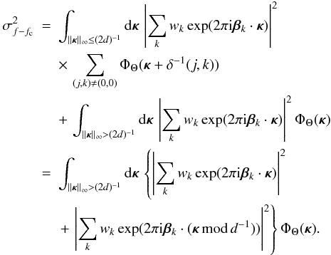 (26)Here
κmod d-1 is the
component-wise remainder of κ when divided by
d-1. Equation (26) is a somewhat awkward expression, and we will only evaluate it explicitly for
the calibration error C (i.e.,
f = Θ) as opposed to
ΔC.
(26)Here
κmod d-1 is the
component-wise remainder of κ when divided by
d-1. Equation (26) is a somewhat awkward expression, and we will only evaluate it explicitly for
the calibration error C (i.e.,
f = Θ) as opposed to
ΔC.
5. Specializing to circular apertures and fields
The special case of a circular, unobscured aperture function
A(r) and a circular science FoV
Ω(α) is generally sufficient for error budgeting purposes.
The Fourier transform of the function
A(r)r
appearing in Eq. (15) then takes the form
=\frac{iD^3J_2(\pi D\nu)}{4D\nu} \left(\begin{array}{c}\cos\phi \\ \sin\phi\end{array}\right), \label{eq27} \end{equation}](/articles/aa/full_html/2013/04/aa21092-13/aa21092-13-eq78.png) (27)where D is
the aperture diameter, J2 is a Bessel function of the first
kind, and φ is the angle of the vector ν.
Substituting Eq. (27) back into Eq. (16) now yields
(27)where D is
the aperture diameter, J2 is a Bessel function of the first
kind, and φ is the angle of the vector ν.
Substituting Eq. (27) back into Eq. (16) now yields 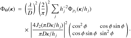 (28)For
a circular FoV of radius ρ, it is reasonable to decompose the image
distortion profile in terms of the orthonormal basis functions
(28)For
a circular FoV of radius ρ, it is reasonable to decompose the image
distortion profile in terms of the orthonormal basis functions 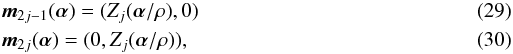 where
the functions Zi are the orthonormal Zernike
polynomials on the unit radius disk as used by Noll
(1976). Using Eq. (21) and Noll’s
formulas for ℱ(Zi) in terms of Bessel
functions, we obtain the result
where
the functions Zi are the orthonormal Zernike
polynomials on the unit radius disk as used by Noll
(1976). Using Eq. (21) and Noll’s
formulas for ℱ(Zi) in terms of Bessel
functions, we obtain the result ![Mathematical equation: \begin{eqnarray} \label{eq31} \lefteqn{\sum_j \left\langle\left[\frac{\int {\rm d}{\bm\alpha}\,\vec{m}_j^T({\bm\alpha})\vec{f}({\bm\alpha})\Omega({\bm\alpha})}{ \int {\rm d}{\bm\alpha}\,\Omega({\bm\alpha})}\right]^2\right\rangle =} \nonumber \\ & & \qquad\qquad\int {\rm d}{\bm\kappa}\,\mbox{Tr}\Phi_f({\bm\kappa})\sum_{n=0}^N \left\vert\frac{(n+1)J_{n+1}(2\pi\rho\kappa)}{\pi\rho\kappa}\right\vert^2 \end{eqnarray}](/articles/aa/full_html/2013/04/aa21092-13/aa21092-13-eq86.png) (31)for
the projection of the function f onto the first
N radial orders of the distortion modes. For example,
N = 0 corresponds to global tip/tilt removal, N = 1 adds
modes for plate scale, animorphic plate scale, and image rotation, and so on.
(31)for
the projection of the function f onto the first
N radial orders of the distortion modes. For example,
N = 0 corresponds to global tip/tilt removal, N = 1 adds
modes for plate scale, animorphic plate scale, and image rotation, and so on.
6. Final formulas and sample numerical results
Using the general results developed in Sects. 3 through 5 above, we can now derive and evaluate expressions for the three error terms of quasi-static distortion, beam wander across static surface distortions, and calibration undersampling error.
6.1. Quasi-static errors
In Sect. 2, the position estimation error due to the
effects of the quasi-static optics figure error q is denoted
Q, and the residual error after low-order mode removal
is written as PQ. This corresponds to the
case f = Θ, and by Eq. (19) the particular value of the LoS error
o + δ is unimportant.
Substituting Eqs. (20), (28), and (31) into Eq. (10)
yields the result 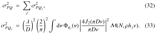 Here
Here
 is the
mean-square position estimation error due to the surface errors on optical surface number
j at conjugate range hj,
D is the aperture diameter, ρ is the diameter of the
FoV,
ν = κ/hj,
and the mode removal filter ℳ is defined by
is the
mean-square position estimation error due to the surface errors on optical surface number
j at conjugate range hj,
D is the aperture diameter, ρ is the diameter of the
FoV,
ν = κ/hj,
and the mode removal filter ℳ is defined by 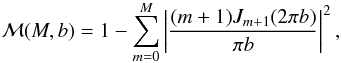 (34)where
M is the maximum radial order of the modes removed from the image
distortion map.
(34)where
M is the maximum radial order of the modes removed from the image
distortion map.
Quasi-static wavefront errors are unpredictable almost by definition, so reliable
information on their PSD may not necessarily be available. However, it is still possible
to develop a “sensitivity” function to describe the magnitude of the error introduced by
one unit of rms wavefront error as a function of spatial frequency. For the higher-order,
tip/tilt/piston removed wavefront errors, this sensitivity function is given by the
formula ![Mathematical equation: \begin{equation} T_{PQ_j}({\bm\nu})=\left(\frac{\lambda}{D}\right)\left(\frac{2}{\pi}\right)\left\vert\frac{4J_2(\pi D\nu)}{\pi D\nu}\right\vert \left[{\cal M}(N,\rho h_j\nu)/{\cal M}(1,D\nu)\right]^{1/2}, \label{eq35} \end{equation}](/articles/aa/full_html/2013/04/aa21092-13/aa21092-13-eq98.png) (35)where the factor of
ℳ(1,Dν) is included to filter out the tip/tilt/piston modes of the
wavefront error on a circular aperture of diameter D.
(35)where the factor of
ℳ(1,Dν) is included to filter out the tip/tilt/piston modes of the
wavefront error on a circular aperture of diameter D.
Figure 1 plots this sensitivity function (in units of μas per nm) for quasi-static wavefront errors on the deformable mirror DM11.2 in the NFIRAOS first light AO system for the Thirty Meter Telescope (Herriot et al. 2012). The relevant parameter values for this instrument are D = 30 m, ρ = 30 arcsec, hj = 11.2 km, and N = 0 or 1. The maximum value of the sensitivity function is approximately 3 μas nm-1 with global tip-tilt removal (N = 0), and approximately 0.15 assuming that the plate scale and rotation modes (N = 1) can also be calibrated using reference stars. Results such as this can be used to help specify the requirements on deformable mirror stability in AO systems used for high precision astrometry.
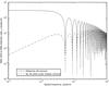 |
Fig. 1 Sensitivity function relating quasi-static wavefront errors on the deformable mirror DM11.2 in the TMT AO system NFIRAOS to the resulting image distortion after low-order mode correction using reference stars. See the text for further parameter values. |
Finally, if the random quasi-static wavefront aberrations have the same variance and are
uncorrelated for two separate science exposures, the value of the differential error due
to the two independent quasi-static errors in two images is simply  (36)
(36)
6.2. Error due to beam wander effects
The position estimation error in a single exposure due to a beam wander across the
optical surface errors is the function
W(α) defined as the first
term within square brackets in Eq. (3).
Using Eqs. (10), (20), (19), (16) and (31) above, we can again evaluate the
mean-square value of the error as sum of contributions from each optical surface, with
each contribution expressed as a weighted integral of the surface error PSD. For a fixed
value of the beam wander δ, the contribution from surface
number j is given by the formula ![Mathematical equation: \begin{eqnarray} \label{eq37} \sigma_{PW_j}^2({\bm\delta}) & = & \left(\frac{\lambda}{D}\right)^2\left(\frac{2}{\pi}\right)^2 \int {\rm d}{\bm\nu}\,\Phi_{s_j}({\bm\nu})\left\vert\frac{4J_2(\pi D\nu)}{\pi D\nu}\right\vert^2 \nonumber \\[-0.5mm] & & \times 2\Re\left[1-\exp(2\pi {\rm i} h_j{\bm\nu}\cdot{\bm\delta})\right]{\cal M}(N,\rho h_j\nu). \end{eqnarray}](/articles/aa/full_html/2013/04/aa21092-13/aa21092-13-eq107.png) (37)If
the beam wander vector is treated as a zero-mean, normally distibuted random error, the
expected error averaged over all realizations of δ is then
given by
(37)If
the beam wander vector is treated as a zero-mean, normally distibuted random error, the
expected error averaged over all realizations of δ is then
given by ![Mathematical equation: \begin{eqnarray} \sigma_{PW_j}^2 & = & 2\left(\frac{\lambda}{D}\right)^2\left(\frac{2}{\pi}\right)^2 \int {\rm d}{\bm\nu}\,\Phi_{s_j}({\bm\nu})\left\vert\frac{4J_2(\pi D\nu)}{\pi D\nu}\right\vert^2 \nonumber \\[-0.5mm] & & \times\left[1-\exp(-2\pi^2 h_j^2\nu^2\sigma_\delta^2)\right]{\cal M}(N,\rho h_j\nu), \label{eq38} \end{eqnarray}](/articles/aa/full_html/2013/04/aa21092-13/aa21092-13-eq108.png) (38)where
σδ is the one-axis rms value of the beam
wander.
(38)where
σδ is the one-axis rms value of the beam
wander.
A common functional form for the fabrication errors on an optical surface is a
(two-dimensional) power law PSD,
Φ(ν) = cν−p.
If the optical surface is specified to have a piston-tip/tilt-focus removed rms OPD equal
to σOPD on a clear aperture of radius equivalent to
RC for the image of the surface in telescope object space,
the coefficient c may be evaluated with the result 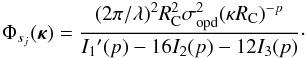 (39)Here the
quantities I1′(p) and
In(p) are similar to the
integrals computed by Noll (1976) for the case of
Kolmogorov turbulence with p = 11/3, and are given by
the expressions
(39)Here the
quantities I1′(p) and
In(p) are similar to the
integrals computed by Noll (1976) for the case of
Kolmogorov turbulence with p = 11/3, and are given by
the expressions ![Mathematical equation: \begin{eqnarray} \label{eq40} I_1\arcmin (p)\! & = & \!\frac{\pi^p \Gamma(p+1)}{ \left\{\Gamma\left[(p\!+\!2)/2\right]\right\}^2\Gamma[(p\!+\!4)/2]\Gamma(p/2)\sin\left[\pi(p\!-\!2)/2\right]} \\ \label{eq41} I_n(p) & = & \frac{\pi^{p-1}\Gamma(p+1)\Gamma[(2n-p)/2]}{4\left\{\Gamma[(p+2)/2]\right\}^2\Gamma[(2n+2+p)/2]}\cdot \end{eqnarray}](/articles/aa/full_html/2013/04/aa21092-13/aa21092-13-eq118.png) By
substituting Eq. (39) into Eq. (38) and applying the change of variable
ν → Dν,
we finally obtain
By
substituting Eq. (39) into Eq. (38) and applying the change of variable
ν → Dν,
we finally obtain ![Mathematical equation: \begin{eqnarray} \label{eq42} \sigma_{PW_j}^2 & = & \frac{64\pi (D/R_{\rm C})^{p-2}(\sigma_{\mbox{opd}}/D)^2}{I_1\arcmin (p)-16I_2(p)-12I_3(p)} \int_0^\infty {\rm d}\nu\,\nu^{1-p}\left\vert\frac{4J_2(\pi \nu)}{\pi\nu}\right\vert^2 \nonumber \\ & & \times\, {\cal M}(N,h_j\rho\nu/D)\left\{1-\exp\left[-2\pi^2\nu^2(h_j\sigma_\delta/D)^2\right]\right\}. \end{eqnarray}](/articles/aa/full_html/2013/04/aa21092-13/aa21092-13-eq120.png) (42)Equation (42) suggests the definition of a normalized
sensitivity coefficient
sPWj
according to the formula
(42)Equation (42) suggests the definition of a normalized
sensitivity coefficient
sPWj
according to the formula ![Mathematical equation: \begin{equation} s_{PW_j}=\sigma_{PW_j}/[(D/R_{\rm C})^{(p-2)/2}(\sigma_{\rm{OPD}}/D)]. \label{eq42a} \end{equation}](/articles/aa/full_html/2013/04/aa21092-13/aa21092-13-eq122.png) (43)We recall that
D is the diameter of the telescope aperture, the rms optical path error
over the clear aperture of surface j is σOPD,
and the radius of this surface is equivalent to RC when imaged
into telescope object space. The normalization defined in Eq. (43) expresses the fact that the rms image
distortion due to beam wander on surface j will scale linearly with the
rms optical path error within the beamprint (i.e., with
(D/RC)(p − 2)/2σOPD),
and inversely with the diameter of the telescope (D). According to
Eq. (42), the resulting sensitivity
coefficient
sPWj
is a function of the surface error power law p, the order of low-order
mode removal N, the normalized FoV diameter
hρ/D, and the normalized beam
wander
hσδ/D.
(43)We recall that
D is the diameter of the telescope aperture, the rms optical path error
over the clear aperture of surface j is σOPD,
and the radius of this surface is equivalent to RC when imaged
into telescope object space. The normalization defined in Eq. (43) expresses the fact that the rms image
distortion due to beam wander on surface j will scale linearly with the
rms optical path error within the beamprint (i.e., with
(D/RC)(p − 2)/2σOPD),
and inversely with the diameter of the telescope (D). According to
Eq. (42), the resulting sensitivity
coefficient
sPWj
is a function of the surface error power law p, the order of low-order
mode removal N, the normalized FoV diameter
hρ/D, and the normalized beam
wander
hσδ/D.
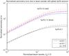 |
Fig. 2 Normalized astrometry error for beam wander with global tip/tilt removed. See Eq. (43) for the definition of this sensitivity coefficient. |
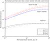 |
Fig. 3 Normalized astrometry error for beam wander with global tip/tilt and plate scale removed. See Eq. (43) for the definition of this sensitivity coefficient. |
The trends in the error due to beam wander across optical surface errors are plotted in Figs. 2 and 3. From the plotted results, we see that
-
Larger random beam wanders always cause larger position estimation errors, although the trend begins to asymptote for normalized jitters beyond the range of 0.3–1.0;
-
Larger fields of view also cause a larger error, although this effect also begins to asymptote for normalized fields of view greater than about 1.0. This result implies that surface errors on optics located far from a pupil (i.e., with a large absolute value of h) have the greatest impact on astrometric accuracy.
-
The expontent of the PSD power law has a relatively smaller effect, with a steeper PSD (more negative exponent) generally yielding a modestly larger error;
-
The error is always reduced by removing the plate scale modes from the image distortion profile, with a greater reduction obtained for smaller normalized fields of view.
![Mathematical equation: \begin{eqnarray} \sigma_{P(\Delta W)_j}^2 & = & \frac{64\pi (D/R_{\rm C})^{p-2}(\sigma_{\mbox{opd}}/D)^2}{I_1\arcmin (p)-16I_2(p)-12I_3(p)} \int_0^\infty {\rm d}\nu\,\nu^{1-p}\left\vert\frac{4J_2(\pi \nu)}{\pi\nu}\right\vert^2 \nonumber \\ & & \times\, {\cal M}(N,h_j\rho\nu/D) \left\{2-2\exp\left[-2\pi^2\nu^2\left(\frac{h_j\sigma_\delta}{D}\right)^2\right]\right. \nonumber \\ & & \left.-\,J_0\left(\frac{2\pi\nu\vert \vec{o}-\vec{o}\arcmin \vert}{D}\right) \left\{1-\exp\left[-2\pi^2\nu^2\left(\frac{h_j\sigma_\delta}{D}\right)^2\right]\right\}^2\right\}\cdot \nonumber \\ & & \label{eq43} \end{eqnarray}](/articles/aa/full_html/2013/04/aa21092-13/aa21092-13-eq128.png) (44)If
the two offset vectors o and
o′ are identical, it may be verified that this expression
simplifies to Eq. (42) with
σδ replaced by
(44)If
the two offset vectors o and
o′ are identical, it may be verified that this expression
simplifies to Eq. (42) with
σδ replaced by
 (as expected).
6.3. Calibration undersampling error
The last two terms to consider are the calibration errors C
and ΔC. The function f
consists of only a single term for C, but two terms for
ΔC. On account of Eq. (26), this means that the formula for
 is much less
tractable than for
is much less
tractable than for  , so we have
only considered the simpler case of the error in a single exposure1.
, so we have
only considered the simpler case of the error in a single exposure1.
Substituting Eq. (39) for a power law PSD
into Eq. (26), the formula for the
mean-square calibration error due to surface number j becomes
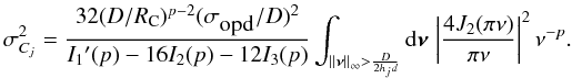 (45)Note that domain of
integration is still two-dimensional, consisting of all spatial frequency vectors
ν with
||ν||∞ = max(ν1,ν2) > (2hjd/D)-1.
Since the integrand in Eq. (45) is
radially symmetric, we replace the square “hole” in the domain of integration with an
equal-area disk so that the integral can be converted into polar coordinates and simplied.
The final formula for the calibration error becomes
(45)Note that domain of
integration is still two-dimensional, consisting of all spatial frequency vectors
ν with
||ν||∞ = max(ν1,ν2) > (2hjd/D)-1.
Since the integrand in Eq. (45) is
radially symmetric, we replace the square “hole” in the domain of integration with an
equal-area disk so that the integral can be converted into polar coordinates and simplied.
The final formula for the calibration error becomes 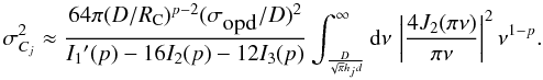 (46)Figure 4 plots the calibration error sensitivity coefficient
![Mathematical equation: \begin{equation} s_{C_j}=\sigma_{C_j}/[(D/R_{\rm C})^{(p-2)/2}(\sigma_{\rm{OPD}}/D)], \label{eq45a} \end{equation}](/articles/aa/full_html/2013/04/aa21092-13/aa21092-13-eq136.png) (47)as a function of
the calibration Nyquist frequency
D/(hjd)
for several different power laws p. We see that for calibration to
provide a meaningful improvement, the calibration Nyquist frequency must exceed 1, or
equivalently the reference source spacing d must satisfy
d < D/hj.
The rms error then falls as the Nyquist frequency to the power
−(p + 1)/2, as would be expected from Eq. (46) and the asymptotic behavior of the Bessel
function J2. Smoother optical surface errors, with larger
values of p, are consequently easier to calibrate.
(47)as a function of
the calibration Nyquist frequency
D/(hjd)
for several different power laws p. We see that for calibration to
provide a meaningful improvement, the calibration Nyquist frequency must exceed 1, or
equivalently the reference source spacing d must satisfy
d < D/hj.
The rms error then falls as the Nyquist frequency to the power
−(p + 1)/2, as would be expected from Eq. (46) and the asymptotic behavior of the Bessel
function J2. Smoother optical surface errors, with larger
values of p, are consequently easier to calibrate.
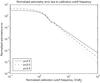 |
Fig. 4 Normalized rms position estimation error due calibration undersampling. See Eq. (47) for the definition of this sensitivity coefficient. |
7. Conclusions
We have derived a Fourier domain model for evaluating the position estimation errors due to optical surface errors in astronomical instrumentation and associated adaptive optics systems. Using analytical methods very similar to those used earlier to study adaptive optics, the errors can be evaluated as a sum of weighted integrals of the surface error PSD on each optical element. Separate formulas have been developed for: (i) quasi-static surface errors; (ii) the error due to beam wander across static surface errors; and (iii) the calibration undersampling error for a finite number of bright, regularly spaced reference sources. The benefits of on-sky calibration using a number of known reference stars in the science image has also been modeled. It is hoped that these results may be useful for developing optical surface specifications and astrometry error budgets.
There are several aspects of this basic model which could be revisited for greater generality and improved accuracy. Characterizing quasi-static surface errors in terms of a PSD may be challenging, since these errors are difficult to model almost by definition. The assumption that surface errors are uncorrelated between different optical surfaces will not necessarily apply to MCAO system, although these correlations will not matter in the important special case that only the ground-layer DM is adjusted to compensate for the static errors on other surfaces. Finally, the current model for calibration, which is based upon a grid of regularly spaced, bright reference sources, is restricted to laboratory source simulators and cannot be used to evaluate the performance of more sophisticated on-sky calibration methods using images of dense star fields. It remains to be seen whether Fourier domain methods are applicable in these cases with an acceptable level of accuracy, or if more computationally intensive approaches such as Monte Carlo simulations may be required instead.
According to Eq. (7), the error ΔC is identically zero if the offset vectors o and o′ are identical.
Acknowledgments
The basic model for astrometry errors described in Sect. 2 above was developed in conversations with Glen Herriot and Matthias Schoeck, and we would also like to thank the referee for providing many helpful suggestions in his review. The TMT Project gratefully acknowledges the support of the TMT collaborating institutions. They are the Association of Canadian Universities for Research in Astronomy (ACURA), the California Institute of Technology, the University of California, the National Astronomical Observatory of Japan, the National Astronomical Observatories of China and their consortium partners, and the Department of Science and Technology of India and their supported institutes. This work was supported as well by the Gordon and Betty Moore Foundation, the Canada Foundation for Innovation, the Ontario Ministry of Research and Innovation, the National Research
Council of Canada, the Natural Sciences and Engineering Research Council of Canada, the British Columbia Knowledge Development Fund, the Association of Universities for Research in Astronomy (AURA) and the US National Science Foundation.
References
- Cameron, P. B., Britton, M. C., & Kulkarni, S. R. 2009, AJ, 137, 83 [Google Scholar]
- Ellerbroek, B. L. 2009, in Adaptive Optics: Methods, Analysis and Applications, eds. B. L. Ellerbroek, & J. Christou (Washington D.C.: OSA) [Google Scholar]
- Fritz, T., Gillessen, S., Trippe, S., et al. 2010, MNRAS, 401, 1177 [NASA ADS] [CrossRef] [Google Scholar]
- Herriot, G., Andersen, D., Atwood, J., et al. 2012, in Adaptive Optics Systems III, eds. B. L. Ellerbroek, E. Marchetti, & J.-P. Veran (Bellingham: SPIE), 84471 [Google Scholar]
- Jolissaint, L., Veran, J.-P., & Conan, R. 2006, J. Opt. Soc. Am A, 23, 382 [NASA ADS] [CrossRef] [Google Scholar]
- Lawson, J. K., Wolfe, C. R., Manes, K. R., et al. 1995, in Optical Manufacturing and Testing, eds. V. J. Doherty, & H. P. Stahl (Bellingham: SPIE), 38 [Google Scholar]
- Lazorenko, P. F., Mayor, M., Dominik, M., et al. 2009, A&A, 505, 903 [NASA ADS] [CrossRef] [EDP Sciences] [Google Scholar]
- Noll, R. J. 1976, J. Opt. Soc. Am., 66, 207 [NASA ADS] [CrossRef] [Google Scholar]
- Roddier, F., Northcott, M. J., Graves, J. E., McKena, D. L., & Roddier, D. 1993, J. Opt. Soc. Am. A, 10, 957 [Google Scholar]
- Schoeck, M. 2011, in Adaptive Optics for Extremely Large Telescopes 2, eds. J.-P. Veran, T. Fusco, & Y. Clenet (Paris: ONERA), 721 [Google Scholar]
- Trippe, S., Davies, R., Eisenhauer, F., et al. 2010, MNRAS, 402, 1126 [NASA ADS] [CrossRef] [Google Scholar]
- Yelda, S., Lu, J. R., Ghez, A. M., et al. 2010, ApJ, 725, 331 [NASA ADS] [CrossRef] [Google Scholar]
All Figures
|
Fig. 1 Sensitivity function relating quasi-static wavefront errors on the deformable mirror DM11.2 in the TMT AO system NFIRAOS to the resulting image distortion after low-order mode correction using reference stars. See the text for further parameter values. |
| In the text | |
|
Fig. 2 Normalized astrometry error for beam wander with global tip/tilt removed. See Eq. (43) for the definition of this sensitivity coefficient. |
| In the text | |
|
Fig. 3 Normalized astrometry error for beam wander with global tip/tilt and plate scale removed. See Eq. (43) for the definition of this sensitivity coefficient. |
| In the text | |
|
Fig. 4 Normalized rms position estimation error due calibration undersampling. See Eq. (47) for the definition of this sensitivity coefficient. |
| In the text | |
Current usage metrics show cumulative count of Article Views (full-text article views including HTML views, PDF and ePub downloads, according to the available data) and Abstracts Views on Vision4Press platform.
Data correspond to usage on the plateform after 2015. The current usage metrics is available 48-96 hours after online publication and is updated daily on week days.
Initial download of the metrics may take a while.