© ESO, 2013

1. Introduction

It is rather uncertain which magnetic field can be present in stellar radiation zones but this field can play an important role in many phenomena in stars such as mixing, angular momentum transport, formation of tachocline etc. (see, e.g., Gough & McIntyre 1998; Heger et al. 2005; Eggenberger et al. 2005; Mathis & Zahn 2005). Likely, dynamos cannot operate in radiation zones, where no strong flows are available to sustain a vigorous dynamo action. Possibly, relic magnetic fields acquired by the star at the early stage of evolution can persist there. This type of fields could have formed, for instance, because of differential rotation that could have stretched the lines of a weak primordial seed field into a dominant toroidal field. Since the conductivity is high, the large-scale relic field could survive in the radiation zone during the life-time of a star.

The magnetic field, however, can evolve in a radiation zone also because of the development of various instabilities. For example, the magnetorotational instability could occur if the radiation zone is magnetized and rotates differentially. However, differential rotation is unlikely in radiation zones and, perhaps, can exist only in stellar tachoclines. Over the past decade, instabilities of the stellar tachocline have been extensively studied (see, e.g., Dikpati et al. 2009 and reference therein). The tachocline is thin and its stability properties are rather peculiar. For instance, Gilman & Fox (1997) showed that the tachocline latitudinal shear is unstable to nonaxisymmetric disturbances when a toroidal magnetic field is present. Instabilities in the tachocline have been studied in detail by Dikpati et al. (2009) for a wide range of rotation and toroidal field profiles. Since rotation is rigid in radiation zones, instabilities of the magnetic field most likely are current-driven. These instabilities do not require differential rotation, and they are well studied in cylindrical geometry in the context of laboratory fusion research (see, e.g., Freidberg 1970; Goedbloed 1971; Goedbloed & Hagebeuk 1972; Tayler 1973a,b, 1980). In astrophysical conditions, the instability caused by electric currents might have a number of characteristic features even in cylindrical geometry (see Bonanno & Urpin 2008a,b, 2011). The nonlinear evolution of the Tayler instability was studied by Bonanno et al. (2012), who argued that symmetry-breaking can give rise to a saturated state with nonzero helicity even if the initial state has zero helicity. A production of nonzero helicity is crucial for the dynamo action.

The stability of the spherical magnetic configurations is studied in much less detail. This problem is of particular interest in relation to Ap star magnetism (Braithwaite & Spruit 2004). With numerical simulations Braithwaite & Nordlund (2006) studied the stability of a random initial field. They argued that this field relaxes on a stable mixed magnetic configuration with both poloidal and toroidal components. A study of the magnetic configurations with a predominantly toroidal field is of particular importance for radiation zones because this field can be easily formed by differential rotation at the early evolutionary stage. Numerical modeling by Braithwaite (2006) confirmed that the toroidal field with B_ϕ ∝ s or ∝ s² (s is the cylindrical radius) is unstable to the m = 1 mode, as was predicted by Tayler (1973a). The stability of azimuthal fields has also been studied by Spruit (1999). The author used a heuristic approach to estimate the growth rate and criteria of instability. Unfortunately, many of these estimates and criteria are valid only near the rotation axis and do not apply in the main fraction of the volume of a radiation zone where the stability properties can be qualitatively different (see Zahn et al. 2007). Recently, Bonanno & Urpin (2012) have considered the stability of the toroidal field in radiation zones by making use of a linear analysis and taking into account stratification and thermal conductivity. It is widely believed that stratification can suppress the Tayler instability. Bonanno & Urpin (2012) calculated the growth rate of instability and argued that the stabilizing influence of gravity can never entirely suppress the instability caused by electric currents. However, a stable stratification can essentially decrease the growth rate of instability.

In this paper, we consider the effect of rotation on the stability of magnetic configurations with a predominantly toroidal field. Rotation is often considered as one more factor that can suppress the Tayler instability and stabilize the magnetic configurations. For instance, Spruit (1999) found that the growth rate of the Tayler instability in a rotating star should be on the order of ~ω_A(ω_A/Ω) if Ω ≫ ω_A, where ω_A and Ω are the Alfven frequency and angular velocity of the star, respectively. Stability of the toroidal field in rotating stars has been considered by Kitchatinov (2008), and Kitchatinov & Rüdiger (2008), who argued that the magnetic instability is determined by the threshold field strength at which the instability sets. Estimating this threshold in the solar radiation zone, the authors imposed the upper limit on the magnetic field to be ≈600 G. The stability of the toroidal field in a rotating radiation zone has been studied by Zahn et al. (2007) in the particular case B_ϕ ∝ s. The particular type of oscillatory modes found by these authors is related to rotation and is stable in the nondissipative limit. However, instability can occur in the form of an oscillatory diffusive instability if dissipation is provided by radiative or Ohmic diffusion.

The paper is organized as follows. The basic equations and mathematical formulation of the problem are presented in Sect. 2. This is followed by results of numerical calculations of the growth rate and frequency of the instability in Sect. 3. The paper closes with a summary of the main results and some remarks in Sect. 4.

2. Basic equations

Consider the stability of an axisymmetric toroidal magnetic field in the radiation zone using a high conductivity limit. We work in spherical coordinates (r, θ, ϕ) with the unit vectors (e_r, e_θ, e_ϕ). We assume that the radiation zone rotates with the angular velocity Ω = const. and that the toroidal field depends on r and θ, B_ϕ = B_ϕ(r,θ). If the magnetic field is subthermal (so that the magnetic pressure is lower than the gas pressure), one can apply the incompressible limit for a consideration of low-frequency modes. We conduct the analysis of hydromagnetic modes in the rest frame rather than in the corotating frame. Generally, some rotation-related effects can be missing in this case. Some insights into how hydromagnetic waves behave in the corotating frame can be found in the papers by Hide (1969) and Acheson & Hide (1973). For instance, effects due to the density stratification can be neglected when considering the dispersion relation for hydromagnetic oscillations if the Brunt-Väisälä frequency is much lower than twice the angular velocity. However, the Brunt-Väisälä frequency is basically much higher than the angular velocity in stellar radiation zones and these effects can be neglected.

The MHD equations in the incompressible limit read

$\begin{array}{ccc}& & \frac{\mathit{\partial }{v}}{\mathit{\partial t}}\mathrm{+}\mathrm{(}{v}\mathrm{·}\mathrm{\nabla }\mathrm{)}{v}\mathrm{=}\mathrm{-}\frac{\mathrm{\nabla }\mathit{p}}{\mathit{\rho }}\mathrm{+}{g}\mathrm{+}\frac{\mathrm{1}}{\mathrm{4}\mathit{\pi \rho }}\mathrm{(}\mathrm{\nabla }\mathrm{\times }{B}\mathrm{)}\mathrm{\times }{B}\mathit{,}\\ & & \frac{\mathit{\partial }{B}}{\mathit{\partial t}}\mathrm{-}\mathrm{\nabla }\mathrm{\times }\mathrm{(}{v}\mathrm{\times }{B}\mathrm{)}\mathrm{=}\mathrm{0}\mathit{,}\\ & & \mathrm{\nabla }\mathrm{·}{v}\mathrm{=}\mathrm{0}\mathit{,}\mathrm{\nabla }\mathrm{·}{B}\mathrm{=}\mathrm{0}\mathit{,}\end{array}$where g is gravity. 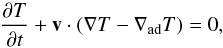The equation of thermal balance reads in the Boussinesq approximation $\frac{\mathit{\partial T}}{\mathit{\partial t}}\mathrm{+}{v}\mathrm{·}\mathrm{(}\mathrm{\nabla }\mathit{T}\mathrm{-}{\mathrm{\nabla }}_{\mathrm{ad}}\mathit{T}\mathrm{)}\mathrm{=}\mathrm{0}\mathit{,}$(4)where ∇_adT is the adiabatic temperature gradient.

In the basic (unperturbed) state, the gas is assumed to be in hydrostatic equilibrium, then 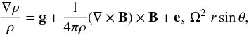$\frac{\mathrm{\nabla }\mathit{p}}{\mathit{\rho }}\mathrm{=}{g}\mathrm{+}\frac{\mathrm{1}}{\mathrm{4}\mathit{\pi \rho }}\mathrm{(}\mathrm{\nabla }\mathrm{\times }{B}\mathrm{)}\mathrm{\times }{B}\mathrm{+}{{e}}_{\mathit{s}}{\mathrm{\Omega }}^{\mathrm{2}}\mathit{r}\sin \mathit{\theta ,}$(5)where e_s is the unit vector in the cylindrical radial direction. The rotational energy is assumed to be much lower than the gravitational one, g ≫ rΩ². The origin and structure of the magnetic field in radiation zones are unknown. However, g is approximately radial in our basic state since we assume that the magnetic energy is subthermal. Only small variations of the density and temperature are required in the meridional direction to balance the centrifugal and Lorentz forces for a given magnetic configuration.

We consider a linear stability. Weak perturbations will be indicated by subscript 1, while unperturbed quantities will have no subscript. Linearizing Eqs. (1)–(4), we take into account that weak perturbations of the density and temperature in the Boussinesq approximation are related by ρ₁/ρ = −β(T₁/T), where β is the thermal expansion coefficient. For weak perturbations, we use a local approximation in the θ-direction and assume that their dependence on θ is proportional to exp (−ilθ), where l ≫ 1 is the longitudinal wavenumber. Since the basic state is stationary and axisymmetric, the dependence of perturbations on t and ϕ can be taken in the exponential form as well. Then, perturbations are proportional to exp (σt − ilθ − imϕ), where m is the azimuthal wavenumber. The corresponding wavevectors are k_θ = l/r and k_ϕ = m/rsinθ, respectively. The dependence on r should be determined from Eqs. (1)–(4).

The problem of the magnetic field stability is complicated from both the physical and computational points of view. The conclusions of different studies are often contradictory (compare, for example, the results by Spruit 1999 and Kitchatinov & Ruediger 2008), and very often the authors do not discuss in detail the reason of the controversy. Because of the complexity of this problem, in our opinion, the best approach is to separately consider the role played by different physical factors (gravity, rotation, conductivity, etc.) in modifying the global structure of the unstable modes. Only after this process has been clarified is it possible to arrive at a global picture of the parameter space. The main motivation of this paper is therefore to clarify the effect of rotation by considering different radial profiles of the toroidal field, in contrast to the study proposed in detail by Bonanno & Urpin (2012), where only the effect of gravity was considered. Therefore, we consider a simplified problem assuming that stratification is neutral and ∇T = ∇_adT. In this case, the stabilizing effect of gravity is neglected and we can study how the instability is affected by rotation alone. For the sake of simplicity, we also assume that the unperturbed density is approximately homogeneous in the radiation zone. As we mentioned above, meridional variations of the density should be small in a subthermal magnetic field. A radial variation is not small in real stars but omitting it does not qualitatively change the main conclusions and substantially simplifies calculations. Eliminating all variables in favor of v_1r, we obtain with the accuracy in terms of the lowest order in (k_θr)^-1

$\begin{array}{ccc}& & \mathrm{(}{\mathit{\sigma }}_{\mathrm{0}}^{\mathrm{2}}\mathrm{+}{\mathit{\omega }}_{\mathrm{A}}^{\mathrm{2}}\mathrm{+}\mathit{D}{{\mathrm{\Omega }}_{\mathrm{i}}^{\mathrm{2}}}^{\mathrm{)}}{\mathit{v}}_{\mathrm{1}\mathit{r}}^{\mathrm{\prime \prime }}\mathrm{+}\left(\frac{\mathrm{4}}{\mathit{r}}{\mathit{\sigma }}_{\mathrm{0}}^{\mathrm{2}}\mathrm{+}\frac{\mathrm{2}}{\mathit{H}}{\mathit{\omega }}_{\mathrm{A}}^{\mathrm{2}}\right){\mathit{v}}_{\mathrm{1}\mathit{r}}^{\mathrm{\prime }}\\ & & \mathrm{+}[\frac{\mathrm{2}}{{\mathit{r}}^{\mathrm{2}}}{\mathit{\sigma }}_{\mathrm{0}}^{\mathrm{2}}\mathrm{-}{\mathit{k}}_{\mathrm{\perp }}^{\mathrm{2}}\mathrm{(}{\mathit{\sigma }}_{\mathrm{0}}^{\mathrm{2}}\mathrm{+}{\mathit{\omega }}_{\mathrm{A}}^{\mathrm{2}}\mathrm{)}\mathrm{-}\mathit{D}{\mathrm{\Omega }}_{\mathrm{e}}^{\mathrm{2}}{\mathit{k}}_{\mathit{\theta }}^{\mathrm{2}}\\ & & \mathrm{+}\frac{\mathrm{2}}{\mathit{r}}{\mathit{\omega }}_{\mathrm{A}}^{\mathrm{2}}\left(\frac{\mathrm{1}}{\mathit{H}}\frac{{\mathit{k}}_{\mathrm{\perp }}^{\mathrm{2}}}{{\mathit{k}}_{\mathit{\varphi }}^{\mathrm{2}}}\mathrm{-}\frac{\mathrm{2}}{\mathit{r}}\frac{{\mathit{k}}_{\mathit{\theta }}^{\mathrm{2}}}{{\mathit{k}}_{\mathit{\varphi }}^{\mathrm{2}}}\mathit{D}\right)\mathrm{-}\mathrm{i}{\mathit{\sigma }}_{\mathrm{0}}{\mathrm{\Omega }}_{\mathrm{e}}\left(\frac{{\mathit{k}}_{\mathit{\varphi }}}{\mathit{r}}\mathrm{+}\mathrm{4}\mathit{D}\frac{{\mathit{k}}_{\mathit{\theta }}^{\mathrm{2}}}{\mathit{r}{\mathit{k}}_{\mathit{\varphi }}}\frac{{\mathit{\omega }}_{\mathrm{A}}^{\mathrm{2}}}{{\mathit{\sigma }}_{\mathrm{0}}^{\mathrm{2}}}\right)]{\mathit{v}}_{\mathrm{1}\mathit{r}}\mathrm{=}\mathrm{0}\mathit{,}\end{array}$(6)where the prime denotes a derivative with respect to r and

$\begin{array}{ccc}& & {\mathit{\sigma }}_{\mathrm{0}}\mathrm{=}\mathit{\sigma }\mathrm{-}\mathrm{i}\mathit{m}\mathrm{\Omega }\mathit{,}{\mathit{\omega }}_{\mathrm{A}}^{\mathrm{2}}\mathrm{=}\frac{{\mathit{k}}_{\mathit{\varphi }}^{\mathrm{2}}{\mathit{B}}_{\mathit{\varphi }}^{\mathrm{2}}}{\mathrm{4}\mathit{\pi \rho }}\mathit{,D}\mathrm{=}\frac{{\mathit{\sigma }}_{\mathrm{0}}^{\mathrm{2}}}{{\mathit{\sigma }}_{\mathrm{0}}^{\mathrm{2}}\mathrm{+}{\mathit{\omega }}_{\mathrm{A}}^{\mathrm{2}}}\mathit{,}\\ & & {\mathrm{\Omega }}_{\mathrm{i}}\mathrm{=}\mathrm{2}\mathrm{\Omega }\cos \mathit{\theta ,}{\mathrm{\Omega }}_{\mathrm{e}}\mathrm{=}\mathrm{2}\mathrm{\Omega }\sin \mathit{\theta ,}{\mathit{k}}_{\mathrm{\perp }}^{\mathrm{2}}\mathrm{=}{\mathit{k}}_{\mathit{\theta }}^{\mathrm{2}}\mathrm{+}{\mathit{k}}_{\mathit{\varphi }}^{\mathrm{2}}\mathit{,}\\ & & \frac{\mathrm{1}}{\mathit{H}}\mathrm{=}\frac{\mathit{\partial }}{\mathit{\partial r}}\ln \mathrm{\left(}\mathit{r}{\mathit{B}}_{\mathit{\varphi }}\mathrm{\right)}\mathit{.}\end{array}$(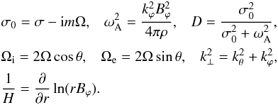7)If Ω = 0, Eq. (6) transforms into the equation derived by Bonanno & Urpin (2012).

Some important stability properties of the toroidal field can be derived directly from Eq. (6). Consider perturbations with a very short radial wavelength for which one can use a local approximation in the radial direction, such as v_1r ∝ exp(−ik_rr), where k_r is the radial wavevector. If k_r ≫ max(k_θ,k_ϕ), then Eq. (6) yields with the accuracy in terms of the lowest order in (k_rr)^-1 the following dispersion equation 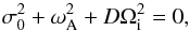${\mathit{\sigma }}_{\mathrm{0}}^{\mathrm{2}}\mathrm{+}{\mathit{\omega }}_{\mathrm{A}}^{\mathrm{2}}\mathrm{+}\mathit{D}{\mathrm{\Omega }}_{\mathrm{i}}^{\mathrm{2}}\mathrm{=}\mathrm{0}\mathit{,}$(8)or ${\mathit{\sigma }}_{\mathrm{0}}^{\mathrm{4}}\mathrm{+}{\mathit{\sigma }}_{\mathrm{0}}^{\mathrm{2}}\mathrm{(}\mathrm{2}{\mathit{\omega }}_{\mathrm{A}}^{\mathrm{2}}\mathrm{+}{\mathrm{\Omega }}_{\mathrm{i}}^{\mathrm{2}}\mathrm{)}\mathrm{+}{\mathit{\omega }}_{\mathrm{A}}^{\mathrm{4}}\mathrm{=}\mathrm{0.}$(9)It is easy to show that this equation has only imaginary roots. Therefore, modes with a short radial wavelength are always stable to the current-driven instability in contrast to the result obtained by Kitchatinov (2008) and Kitchatinov & Rüdiger (2008).

3. Numerical results

We assume that the radiation zone is located at R_i ≤ r ≤ R or, introducing the dimensionless radius x = r/R, at x_i ≤ x ≤ 1 where x_i = R_i/R. We choose the internal radius of the radiation zone, x_i, to be equal to 0.1 from computational reasons. We have verified that our results are basically insensitive to the precise value of x_i as long as it is close to the center.

The toroidal field can be represented as ${\mathit{B}}_{\mathit{\varphi }}\mathrm{=}{\mathit{B}}_{\mathrm{0}}\mathit{\psi }\mathrm{\left(}\mathit{x}\mathrm{\right)}\sin \mathit{\theta ,}$(10)where B₀ is the characteristic field strength and ψ ~ 1 is a function of the spherical radius alone. The dependence of ψ on x is uncertain in the radiation zone and, in this paper, we consider three different possibilities. Figure 1 plots the profiles ψ(x) for the models (1), (2), and (3) used in our calculations. The case where the field reaches its maximum at the outer boundary (model (2)) can mimic, for example, the radiation zone of a star with a convective envelope. In this case, the bottom of a convection zone likely is the location of the toroidal field generated by a dynamo action. The toroidal field can penetrate into the radiation zone, for instance, because of diffusion. Model (2) can also mimic the toroidal field in the liquid core of neutron stars. Likely, the magnetic field of these objects is generated by turbulent dynamo during the very early phase of evolution when the neutron star is subject to hydrodynamical instabilities (see Bonanno et al. 2005, 2006). A large-scale dynamo is most efficient in the surface layers where the density gradient is highest. Therefore, the generated field increases outward and reaches its maximum in the outer layers (Bonanno et al. 2005, 2006). This magnetic field can be subject to current-driven instabilities after the end of the initial phase. Note that dynamo induced by turbulent motions generates not only a large-scale field but also small-scale fields of complex topology (Urpin & Gil 2004). The stability properties of the configurations with mixed small- and large-scale fields can be very particular and are not studied yet. The model (3) with a decreasing toroidal field can mimic a star whose magnetic field is generated in the inner convective core. Generally, all three models (1), (2), and (3) can be representative of the stars with relic magnetic fields because the details of the formation of these fields are very uncertain.

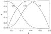Fig. 1 Dependence of the toroidal field on the spherical radius for models (1), (2), and (3).

Introducing the dimensionless quantities as $\mathrm{\Gamma }\mathrm{=}\frac{{\mathit{\sigma }}_{\mathrm{0}}}{{\mathit{\omega }}_{\mathrm{A}\mathrm{0}}}\mathit{,\eta }\mathrm{=}\frac{\mathrm{2}\mathrm{\Omega }}{{\mathit{\omega }}_{\mathrm{A}\mathrm{0}}}\mathit{,}$(11)where ${\mathit{\omega }}_{\mathrm{A}\mathrm{0}}^{\mathrm{2}}\mathrm{=}{\mathit{B}}_{\mathrm{0}}^{\mathrm{2}}\mathit{/}\mathrm{4}\mathit{\pi \rho }{\mathit{R}}^{\mathrm{2}}$, we can transform Eq. (6) into a dimensionless form. This equation with the corresponding boundary conditions describes the stability problem as a nonlinear eigenvalue problem. Fortunately, the main qualitative features of this problem are not sensitive to the choice of boundary conditions. That is why we choose the simplest boundary conditions and assume that v_1r = 0 at r = R_i and r = R. Generally, solutions of Eq. (6) are complex. It is more convenient to split all quantities into the real and imaginary parts and to solve numerically the set of two real coupled equations that follows from Eq. (6). Note that coefficients of Eq. (6) and the corresponding dimensionless equation depend on θ, which in turn leads to the dependence of Γ on it.

The stability properties in the spherical geometry are qualitetively different from those in the cylindrical geometry (see Bonanno & Urpin 2012). Therefore, the results obtained, for instance, for the toroidal field dependending on the cylindrical radius alone (see Spruit 1999; Zhang et al. 2003) does not apply to more general magnetic configurations. The stability problem becomes particularly complex if the radiation zone rotates.

In Fig. 2, we plot the growth rate and frequency of the Tayler modes as functions of η at different θ for the model (2). Like the case of a non-rotating star, the Tayler instability is the most efficient at the equator (see also Bonanno & Urpin 2012). At small η, the growth rate is of the order of 1.4ω_A0 but it clearly shows some suppression for a faster rotation. Suppression becomes significant already at relatively low values of η ~ 2−3. The growth rate decreases with an increase of η approximately as 1/η and it does not vanish even at very large η. A similar behavior was obtained by Spruit (1999), who considered the instability near the rotation axis for B_ϕ = B_ϕ(s). It turns out that rotation can never entirely suppress the Tayler instability of model (2) but only decreases the growth rate. Tayler modes are oscillatory in a rotating radiation zone in contrast to the nonrotating case. The frequency is basically comparable to the growth rate and also decreases when the rotation becomes faster.

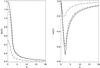Fig. 2 Growth rate (left panel) and frequency (right panel) of the Tayler modes as functions of the rotational parameter η for θ = π/2 (solid), π/6 (dashed), and π/10 (dash-and-dotted) and for model (1). The longitudinal and azimuthal wavenumbers are l = 10 and m = 1, respectively.

Figure 3 shows the results of calculations of the growth rate and frequency for model (1). The results are very similar to those obtained for model (2). As in the previous case, the instability is most efficient at the equator and its growth rate decreases when it approaches the rotation axis. This result is at variance with the widely accepted opinion that toroidal magnetic configurations are always unstable at the axis (see, e.g., Spruit 1999). This opinion is usually based on the similarity of the spherical magnetic configuration near the axis and the axisymmetric cylindrical configuration. However, this analogy is generally incorrect because in spherical geometry, the toroidal field near the axis also depends on the radial coordinate along the axis. Therefore, it can be unjustified to apply the results obtained for a cylinder with B_ϕ = B_ϕ(s) to the case of plasma near the symmetry axis in spherical geometry (Bonanno & Urpin 2012). Indeed, in the latter case stability can crucially depend on the profile of the toroidal field along the symmetry axis. Like model (2), the instability of model (1) is strongly suppressed by rotation. Suppression becomes essential at η ≥ 3−4. At large η, the growth rate decreases ∝1/η, as in the previous case. The stabilization cannot be reached at any large η but the growth rate can be substantially reduced.

Fig. 3 Same as in Fig. 2 but for model (2).

In Fig. 4, we plot the growth rate and frequency as functions of η for model 3. Magnetic configurations with a rapidly decreasing toroidal field are stable in a cylindrical geometry. For example, stability properties of the toroidal field are determined by the parameter α = dlnB_ϕ(s)/dlns. The field is unstable to axisymmetric perturbations if α > 1 and to nonaxisymmetric perturbations if α > −1/2 (Tayler 1973a,b, 1980). The situation is qualitatively different in spherical geometry and even the toroidal field, decreasing rapidly with r, can be unstable. Again, the instability is most efficient at the equator. However, its efficiency decreases drastically toward the pole and the instability does not occur in the region around the rotation axis. The critical angle, θ_cr, which distinguishes the stable and unstable regions, is ~40°. At variance with the models (1) and (2), the instability of the model (3) is determined by the threshold field strength. The threshold is not very high and corresponds to η ≈ 7. Therefore, the Tayler instability is entirely suppressed in model (3) if Ω ≳ 3.5ω_A0. The growth rate is vanishing everywhere in the radiation zone for more rapidly rotating stars.

Fig. 4 Same as in Fig. 2 but for model (3) and θ = π/2 (solid) and π/3 (dashed).

4. Conclusion

We have considered the stability of the toroidal field in rotating stellar radiation zones. The stability properties of the spherical magnetic configurations turn out to be qualitatively different from those of the cylindrical configurations (Bonanno & Urpin 2012). For instance, in contrast to widely accepted opinion, the toroidal field can be stable even near the symmetry axis. The reason for this behavior is the spatial dependence of the magnetic field along the axis, which can provide a stabilizing effect. Therefore, a direct analogy between the stability of a cylinder with the azimuthal field and the toroidal field near the axis in radiation zones is generally incorrect.

Rotation provides a stabilizing effect on the Tayler instability. The effect of rotation can be characterized by the parameter η, which is generally large in radiation zones. It turns out that the effect of rotation depends critically on the magnetic configuration. If the toroidal field increases with the spherical radius within the radiation zone (or some fraction of it, see models (1) and (2)) then rotation cannot entirely suppress the Tayler instability even at very large η. The instability growth rate is discernible for any rotation but can be substantially reduced at very large η. A reduction of the growth rate becomes important even at a relatively low angular velocity Ω ~ 2−3ω_A0. At large η, the growth rate behaves like ω_A0(ω_A0/Ω), as was obtained by Spruit (1999) for a particular case B_ϕ = B_ϕ(s) near the rotation axis. The Alfven timescale, ${\mathit{\omega }}_{\mathrm{A}\mathrm{0}}^{-1}$, is short compared to the stellar life-time, therefore even a suppressed instability with a reduced growth rate can be significant for radiation zones. It should be noted also that, most likely, the field does not decay to zero because of this instability. When the field becomes weaker, the growth rate of the instability decreases and the field cannot decay to values lower than those resulting from the condition that the growth rate is on the order of the inverse life-time of a star. Therefore, a weak field can change only insignificantly during the life of the star, although its radial profile can be unstable.

If the toroidal field decreases with the spherical radius (see Fig. 4 for model (3)), the rotation effect is different. In contrast to models (1) and (2), the instability of model (3) is determined by the threshold field strength. The threshold is not very high and corresponds to η ≈ 7. Therefore, the Tayler instability is entirely suppressed in the model (3) if Ω ≳ 3.5ω_A0 and modes are stable everywhere in the radiation zone for more rapidly rotating stars. Higher eigenmodes are suppressed more strongly than the fundamental one and perturbations with a short radial wavelength are always stable. Since instability is not suppressed at η < 7, this implies that the magnetic field should satisfy the condition ${\mathit{B}}_{\mathrm{0}}\gtrsim \mathrm{0.3}\mathrm{\Omega }\mathit{R}\sqrt{\mathrm{4}\mathit{\pi \rho }}$. Estimating ΩR ~ 2 × 10⁵ cm/s and ρ ~ 0.1 g/cm³, we obtain that instability can arise in the radiation zone of the Sun if B₀ ≳ 7 × 10⁴ G. This estimate is more than two orders of magnitude higher than that obtained by Kitchatinov & Rüdiger (2008). These authors considered stability of the toroidal field assuming that perturbations are global in the meridional direction and short-scaled in radius. As a result, they obtained that the most rapidly growing modes modes are indefinitely short in the radial direction if diffusion is neglected. This conclusion is questionable because simple analytic considerations (see Sect. 2 of the present paper) show that perturbations with short radial wavelength should always be stable. In particular our numerical calculations also show that the fundamental eigenmode has a higher growth rate than higher eigenmodes.

Finally, we calculated the growth rate assuming a neutral stratification of the radiation zone. If the stratification is stable, gravity provides an additional stabilizing influence on the Tayler instability, as was argued by Bonanno & Urpin (2012).

Therefore, suppression of the instability can be even more pronounced and the calculated growth rates are likely to be only upper limits in real, magnetized stellar interiors.

Acknowledgments

V.U. acknowledges support from the European Science Foundation (ESF) within the framework of the ESF activity “The New Physics of Compact Stars”. V.U. also thanks the Russian Academy of Sciences for financial support under the program OFN-15 and the INAF-Ossevatorio Astrofisico di Catania for hospitality.

References

All Figures

	Fig. 1 Dependence of the toroidal field on the spherical radius for models (1), (2), and (3).
In the text

	Fig. 2 Growth rate (left panel) and frequency (right panel) of the Tayler modes as functions of the rotational parameter η for θ = π/2 (solid), π/6 (dashed), and π/10 (dash-and-dotted) and for model (1). The longitudinal and azimuthal wavenumbers are l = 10 and m = 1, respectively.
In the text

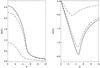	Fig. 3 Same as in Fig. 2 but for model (2).
In the text

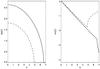	Fig. 4 Same as in Fig. 2 but for model (3) and θ = π/2 (solid) and π/3 (dashed).
In the text

References

- Acheson, D., & Hide, R. 1973, RPPh, 36, 159 [Google Scholar]
- Bonanno, A., & Urpin, V. 2008a, A&A, 477, 35 [NASA ADS] [CrossRef] [EDP Sciences] [Google Scholar]
- Bonanno, A., & Urpin, V. 2008b, A&A, 488, 1 [NASA ADS] [CrossRef] [EDP Sciences] [Google Scholar]
- Bonanno, A., & Urpin, V. 2011, Phys. Rev. E, 84, 6310 [NASA ADS] [CrossRef] [Google Scholar]
- Bonanno, A., & Urpin, V. 2012, ApJ, 747, 137 [NASA ADS] [CrossRef] [Google Scholar]
- Bonanno, A., Urpin, V., & Belvedere, G. 2005, A&A, 440, 199 [NASA ADS] [CrossRef] [EDP Sciences] [Google Scholar]
- Bonanno, A., Urpin, V., & Belvedere, G. 2006, A&A, 451, 1049 [NASA ADS] [CrossRef] [EDP Sciences] [Google Scholar]
- Bonanno, A., Brandenburg, A., Del Sordo, F., & Mitra, D. 2012, Phys. Rev. E, 86, 016313 [NASA ADS] [CrossRef] [Google Scholar]
- Braithwaite, J., & Spruit, H. 2004, Nature, 431, 819 [NASA ADS] [CrossRef] [PubMed] [Google Scholar]
- Braithwaite, J., & Nordlund, A. 2006, A&A, 450, 1077 [NASA ADS] [CrossRef] [EDP Sciences] [Google Scholar]
- Dikpati, M., Gilman, P., Cally, P., & Miesch, M. 2009, 692, 1421 [Google Scholar]
- Eggenberger, P., Maeder, A., & Meynet, G. 2005, A&A, 440, 9 [Google Scholar]
- Freidberg, J. 1970, Phys. Fluids, 13, 1812 [NASA ADS] [CrossRef] [Google Scholar]
- Gilman, P., & Fox, P. A. 1997, ApJ, 484, 439 [NASA ADS] [CrossRef] [Google Scholar]
- Goedbloed, J. P. 1971, Physica, 53, 501 [NASA ADS] [CrossRef] [Google Scholar]
- Goedbloed, J. P., & Hagebeuk, H. J. 1972, Phys. Fluids, 15, 1090 [NASA ADS] [CrossRef] [Google Scholar]
- Gough, D. O., & McIntyre, M. E. 1998, Nature, 394, 755 [NASA ADS] [CrossRef] [Google Scholar]
- Heger, A., Woosley, S., & Spruit, H. 2005, ApJ, 626, 350 [NASA ADS] [CrossRef] [Google Scholar]
- Hide, R. 1969, JFM, 39, 283 [NASA ADS] [CrossRef] [Google Scholar]
- Kitchatinov, L. 2008, Astron. Rep., 52, 247 [NASA ADS] [CrossRef] [Google Scholar]
- Kitchatinov, L., & Rüdiger, G. 2008, A&A, 478, 1 [NASA ADS] [CrossRef] [EDP Sciences] [Google Scholar]
- Mathis, S., & Zahn, J.-P. 2005, A&A, 440, 653 [NASA ADS] [CrossRef] [EDP Sciences] [Google Scholar]
- Spruit, H. 1999, A&A, 349, 189 [NASA ADS] [Google Scholar]
- Tayler, R. 1973a, MNRAS, 161, 365 [NASA ADS] [CrossRef] [Google Scholar]
- Tayler, R. 1973b, MNRAS, 163, 77 [NASA ADS] [CrossRef] [Google Scholar]
- Tayler, R. 1980, MNRAS, 191, 151 [NASA ADS] [Google Scholar]
- Urpin, V., & Gil, J. 2004, A&A, 415, 305 [NASA ADS] [CrossRef] [EDP Sciences] [Google Scholar]
- Zahn, J.-P., Brun, A. S., & Mathis, S. 2007, A&A, 474, 145 [NASA ADS] [CrossRef] [EDP Sciences] [Google Scholar]
- Zhang, K., Liao, X., & Schubert, G. 2003, ApJ, 585, 1124 [NASA ADS] [CrossRef] [Google Scholar]