| Issue |
A&A
Volume 551, March 2013
|
|
|---|---|---|
| Article Number | A13 | |
| Number of page(s) | 6 | |
| Section | Stellar structure and evolution | |
| DOI | https://doi.org/10.1051/0004-6361/201220718 | |
| Published online | 12 February 2013 | |
Structure of the hadron-quark mixed phase in protoneutron stars
1
INFN Sezione di Catania, Dipartimento di FisicaUniversitá di
Catania,
via Santa Sofia 64,
95123
Catania,
Italy
2
Physics Department, China University of Geoscience,
430074
Wuhan, PR
China
3
Yukawa Institute for Theoretical Physics, Kyoto University,
606-8502
Kyoto,
Japan
4
Department of Physics, Chiba Institute of
Technology, 2-1-1 Shibazono,
Narashino, 275-0023
Chiba,
Japan
Received: 12 November 2012
Accepted: 30 December 2012
We study the hadron-quark phase transition in the interior of hot protoneutron stars, combining the Brueckner-Hartree-Fock approach for hadronic matter with the MIT bag model or the Dyson-Schwinger model for quark matter. We examine the structure of the mixed phase constructed according to different prescriptions for the phase transition and the resulting consequences for stellar properties. We find important effects for the internal composition, but only very small influence on the global stellar properties.
Key words: dense matter / equation of state / stars: neutron / stars: evolution
© ESO, 2013
1. Introduction
A protoneutron star (PNS) is formed after the gravitational collapse of the core of a massive star (M ≳ 8 M⊙), exploding in a type-II supernova (Shapiro & Teukolsky 1983; Bethe 1990). Although the explosion mechanism is still not fully explained (Burrows 2012), some general features can be considered as robust. In fact, just after the core bounce, the PNS is very hot and lepton-rich, and neutrinos are trapped for a few seconds. The following evolution of the PNS is dominated by neutrino diffusion, causing deleptonization and subsequently cooling. Ultimately, the neutron star (NS) achieves thermal equilibrium and stabilizes at practically zero temperature without trapped neutrinos.
The theoretical description of the formation of a PNS requires an accurate treatment of the microphysics of the collapsing matter, in particular of neutrino transport and related processes (Burrows & Lattimer 1986; Prakash et al. 1997; Burrows 2012). Moreover the violent dynamical processes occurring in the contracting-exploding star need to be treated in the framework of general relativity (see Ott 2009, for a recent review). The physical processes which contribute to the subsequent PNS evolution, such as nuclear and weak interactions and energy and lepton number transport by neutrino diffusion, are very difficult to include in dynamical simulations. Thus, most simulations of the gravitational core collapse to a PNS end shortly after the core bounce and the launch of the supernova explosion, typically after a few hundreds of milliseconds, and only a few dynamical simulations extend to the first minute of the PNS life (Pons et al. 1999; Fischer & Mueller 2009).
During the evolution of a PNS into a NS, a hadron-quark (HQ) phase transition could take place in the central region of the star (Prakash et al. 1995; Lugones & Benvenuto 1998; Pons et al. 1999, 2001; Steiner et al. 2000; Epsztein Grynberg et al. 2000; Nicotra et al. 2006a; Yasutake et al. 2011), and this would alter substantially the composition of the core. In fact the heaviest NS, close to the maximum mass (about two solar masses), are characterized by central baryon densities larger than 1/fm3, as predicted by calculations based on a microscopic nucleonic equation of state (EOS).
The study of hybrid stars is also important from another point of view: purely nucleonic EOS are able to accommodate fairly large (P)NS maximum masses (Baldo et al. 1997; Akmal et al. 1998; Glendenning 2000; Zhou et al. 2004; Li & Schulze 2008), but the appearance of hyperons in beta-stable matter could strongly reduce this value (Glendenning 2000; Schulze et al. 2006; Li & Schulze 2008; Carroll et al. 2009; Ðapo et al. 2010; Schulze & Rijken 2011). In this case the presence of non-baryonic, i.e., “quark” matter would be a possible manner to stiffen the EOS and reach larger NS masses (Burgio et al. 2002; Maieron et al. 2004; Kurkela et al. 2010; Weissenborn et al. 2011). Heavy NS thus would be hybrid quark stars.
In previous articles (Nicotra et al. 2006b; Burgio & Schulze 2009, 2010; Burgio et al. 2011a) we have studied static properties of PNS using a finite-temperature hadronic EOS including also hyperons (Burgio et al. 2011b) derived within the Brueckner-Bethe-Goldstone theory of nuclear matter (Baldo 1999). An eventual HQ phase transition was modeled within an extended MIT bag model (Nicotra et al. 2006a; Yasutake et al. 2011) or a more sophisticated quark model, the Dyson-Schwinger model (DSM; Roberts & Williams 1994; Roberts & Schmidt 2000; Alkofer & von Smekal 2001; Roberts et al. 2007; Chen et al. 2011, 2012).
The purpose of the present work is to complement our previous articles by studying details of the HQ phase transition occuring in hybrid stars and their implications for the structure of a PNS, in particular the question whether global (P)NS observables are sensitive to and thus may reveal information on the internal stellar structure.
In Sect. 2 we briefly sketch the theoretical approaches which we use for modeling the hadron and the quark phases, and in Sect. 3 we describe the corresponding pure phases. The structure of the mixed phase is discussed in Sect. 4, and the results are illustrated in Sect. 5. Finally, in Sect. 6 we summarize our conclusions.
2. Equations of state
The EOSs for hadronic matter (HM) and quark matter (QM) that we use in this work, have been amply discussed in previous publications (Burgio et al. 2002; Maieron et al. 2004; Nicotra et al. 2006a,b; Burgio & Schulze 2009, 2010; Burgio et al. 2011b; Chen et al. 2011, 2012), where all necessary details can be found. Our hadronic EOS is obtained from Brueckner-Hartree-Fock (BHF) calculations of (hyper)nuclear matter (Schulze et al. 1998; Baldo et al. 1998, 2000) based on realistic potentials (the Argonne V18 nucleon-nucleon, Wiringa et al. 1995; and the Nijmegen NSC89 nucleon-hyperon, Maessen et al. 1989, in this case) supplemented by nucleonic Urbana UIX three-body forces (Carlson et al. 1983; Schiavilla et al. 1986; Pudliner et al. 1997), and extended to finite temperature (Burgio et al. 2011b). We employ two different representative models for QM, an extended MIT bag model (the model with a density-dependent bag constant of Burgio et al. 2002; Maieron et al. 2004; Nicotra et al. 2006a) and a Dyson-Schwinger model (the model DS4 of Chen et al. 2011, 2012), which yield in fact quite different internal structures of hybrid stars.
Those theoretical calculations provide the free energy density of the bulk system (pure HM or QM) as a function of the relevant partial number densities ni and the temperature, f({ni} ,T), from which all thermodynamic quantities of interest can be computed, namely, the chemical potentials μi, pressure p, entropy density s, and internal energy density ε read as  where nB is the total baryon number density. These quantities allow one to determine the stellar matter composition and the EOS, which is the fundamental input for solving the Tolman-Oppenheimer-Volkoff equations of (P)NS structure.
3. Pure phases
In neutrino-trapped beta-stable (hyper)nuclear or quark matter the chemical potential μi of any particle i = n,p,Λ,Σ−,u,d,s,e,μ,νe,νμ,... is uniquely determined by the conserved quantities baryon number Bi, electric charge Ci, and weak charges (lepton numbers)  with the corresponding set of independent chemical potentials μB, μC, μL(e), μL(μ):
  (5)In this work we neglect muons and muon neutrinos due to their low fractions and negligible impact on global stellar properties, hence use simply ν ≡ νe, L ≡ L(e). The relations between chemical potentials and partial densities for hadrons and quarks are given by the microscopic models mentioned before, while leptons are treated as free fermions. With such relations, the bulk system in each phase can be solved for a given baryon density, imposing the charge neutrality condition and lepton number conservation:
  When the neutrinos νe are untrapped, the lepton number is not conserved any more, the density and the chemical potential of νe vanish, and the above equations simplify accordingly.
4. Mixed phase constructions
We are interested in the HQ phase transition in PNS and consider therefore the usual oversimplified standard conditions, namely trapped hot matter with a fixed lepton fraction Ye ≡ (ne + nν)/nB = 0.4 and either an isentropic, S/A = 2, or an isothermal, T = 40 MeV, temperature profile. One could consider more realistic profiles (Burgio et al. 2011a), but we focus in this work on the difference between phase transition constructions.
A fully microscopic treatment of the HQ mixed phase involving finite-size (pasta) structures can only be performed numerically (Tatsumi et al. 2003; Endo et al. 2005, 2006; Maruyama et al. 2007; Yasutake et al. 2009, 2012a,b). One introduces Coulomb energies and surface energies via a HQ surface tension and then minimizes the (free) energy of a Wigner-Seitz (WS) cell, allowing for different geometrical structures of the quark phase embedded in the hadron phase and vice versa. The output are the optimal size and geometry of the cell, as well as the local distributions of the individual particle species, and also the Coulomb field inside the cell. Some illustrative examples can be found in the given references.
This is a very time-consuming and not very transparent numerical procedure. It is therefore convenient to search for reliable approximations to this procedure, and in this article we compare two prescriptions corresponding to two limiting cases of the full numerical procedure, that are termed global charge neutral (GCN) and local charge neutral (LCN) mixed phase.
The first procedure is well known as Bulk Gibbs or Glendenning construction (Glendenning 1992, 2001) from the zero-temperature case and corresponds to a “small” WS cell (compared to the electromagnetic Debye screening length, which is about 5−10 fm, Heiselberg et al. 1993; Heiselberg 1993; Glendenning & Pei 1995; Christiansen & Glendenning 1997; Takatsuka et al. 2006) caused by a “small” HQ surface tension. In this case the electromagnetic potential is practically constant throughout the cell, and an electric field does not exist. Consequently the electron density is also constant, while the hadron and quark densities and their electric charges are different in order to fulfill the conditions of pressure and baryon chemical potential equality at the HQ interface. In the case of neutrino trapping, the neutrino densities have also to be equal in both phases,  (9)which together with the equal electron densities implies equal lepton densities nL = ne + nν (but not lepton fractions Ye = nL/nB) in both phases. Altogether we have therefore the equality of the intensive thermodynamical quantities in both phases:
  which together with the general rule Eq. (5) determines the composition of the system for given overall baryon density nB, vanishing electric charge, fixed lepton fraction Ye in the trapped case, and eventually a prescribed entropy profile S/A(nB):
  where χ is the volume fraction occupied by the quark phase and the last equation determines the local temperature.
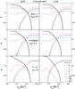 |
Fig. 1 Relative populations xi = ni/nB for different stellar compositions: trapped matter with S/A = 2 (upper panels) or T = 40 MeV (central panels), and untrapped matter with T = 0 (lower panels). The GCN (left panels) or LCN (right panels) construction for the mixed phase is employed together with the MIT bag model for the quark phase. |
The opposite limiting case (LCN) corresponds to a WS cell that is large relative to the electromagnetic Debye screening length, and a large surface tension. In this situation the electric charges are well screened inside the cell and both QM and HM are locally charge neutral nearly everywhere,  (19)except on a small boundary layer near the HQ interface, where a positively charged layer of HM and a negatively charged one of QM are present and create a strong but very localized electric field (Voskresensky 2002; Voskresensky et al. 2003). Consequently there occurs a sharp rise δμC of the Coulomb potential at the HQ interface and Eq. (11) is modified to
  (20)such that for example the electron density is now different in hadron and quark phases.
In beta-stable untrapped matter this situation corresponds exactly to the usual Maxwell construction, joining two charge-neutral phases by equality of pressure and baryon chemical potential, that is often employed for simplicity. Including neutrino trapping with microscopic finite-size structures requires always homogeneous neutrino densities, Eq. (9), and therefore, due to the unequal electron densities, in this case the trapping condition becomes a global one, as expressed by Eq. (17). Due to the additional degree of freedom represented by the neutrino density, then the LCN construction is realized in the PNS as an extended mixed phase involving a HQ coexistence region with a continuously varying pressure (Hempel et al. 2009; Pagliara et al. 2009, 2010; Yasutake et al. 2012b).
We have explained that the GCN and LCN constructions are in fact idealized scenarios that correspond to two opposite extremes of the microscopic treatment. It has been pointed out in Yasutake et al. (2012a,b) that actually the LCN construction is closer to the full microscopic treatment of finite-size effects than the GCN, and it is therefore of interest to compare the predictions of the two constructions for the internal composition and other properties of PNS, which we will do now.
5. Results
5.1. Internal composition
The relative particle populations are shown as a function of the baryon density in Fig. 1 for the bag model and in Fig. 2 for the DSM, for trapped matter with Ye = 0.4 and i) entropy per baryon S/A = 2 (upper panels); ii) temperature T = 40 MeV (middle panels); and iii) untrapped and cold neutron star matter (lower panels). The GCN (left panels) and LCN (right panels) calculations are compared.
There are big differences between the MIT and DSM regarding the HQ mixed phase that have been pointed out in Chen et al. (2011, 2012): with the MIT model the HQ phase transition starts at fairly low baryon density and a pure quark phase is reached at not too large density, whereas with the DSM the onset of the mixed phase occurs at higher density and the system remains in the mixed phase even at very large density. Furthermore, hyperons are allowed with the MIT model, where they might appear only in small fractions at low density and are replaced by strange QM at higher density (this can be seen in the central panels of Fig. 1), whereas they prevent any transition to QM with the DSM and have to be excluded by hand in that case. Therefore, these two very different quark models might be good candidates to reveal important differences between the phase transition constructions that we are examining.
In fact, comparing now the results obtained with both prescriptions (left and right panels), we observe behavior in line with the general properties mentioned before. We remind that for cold NS matter (bottom panels) the LCN corresponds to the usual Maxwell construction and the GCN to the bulk Gibbs construction; and it is well known that the density range of the mixed phase with the Gibbs construction is wider than the one with the Maxwell construction, which can be seen in the plots. This behavior remains also in trapped hot matter, where the GCN spans always a wider density range than the LCN (with the MIT) or begins at lower density (with the DSM). In all cases the trapping condition shifts the onset of the mixed phase to slightly higher density.
The differences between the LCN and GCN constructions are fairly small for the MIT model, but significant for the DSM: here the GCN (Bulk Gibbs) mixed phase occurs in a much wider density interval than the LCN (Maxwell) one. Apart from the Maxwell construction for cold NSs, the matter remains in the mixed phase and pure QM is never reached. This variance is due to the qualitatively different density dependence of the effective bag constant in the MIT and DSM, see Chen et al. (2011, 2012).
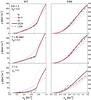 |
Fig. 3 Pressure vs. baryon density for the same stellar configurations as in Fig. 1, and obtained with the MIT (left panels) and the DSM (right panels) quark models. |
5.2. Equation of state
In Fig. 3 the EOS p(nB) is displayed for the different stellar configurations, quark models, and mixed phase constructions as before. For comparison also the pure phases (nucleons only, nucleons+hyperons, quarks) are shown.
We observe only minor differences between GCN and LCN in the hot and trapped matter, even for the DSM, where the particle fractions are quite different in both cases. Stronger differences between GCN and LCN appear in the cold case, where a plateau in the pressure shows up for the LCN (Maxwell) calculation.
Thus if during the temporal evolution the system would remain in the LCN phase, the extended mixed phase region would gradually disappear. However, one should remember that both LCN and GCN are highly idealized constructions and the true behavior depends on currently uncertain microphysics like the HQ surface tension.
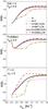 |
Fig. 4 Gravitational mass vs. central baryon density for different stellar configurations and EOS. |
5.3. Stellar structure
Once the EOS is known, the stable configurations of a (P)NS can be obtained from the well-known hydrostatic equilibrium equations of Tolman, Oppenheimer, and Volkov (Shapiro & Teukolsky 1983). In the low-density range, where nucleonic clustering sets in, we cannot use the BHF approach, and therefore we join (Burgio & Schulze 2010) the BHF EOS to the finite-temperature or -entropy EOS of Shen et al. (1998a,b), which is more appropriate at densities below nB ≲ 0.07fm-3, since it does include the treatment of finite nuclei.
Our results for the gravitational mass as a function of the central baryon density, for the different stellar configurations and using the different EOS introduced previously, are displayed in Fig. 4. We observe in NS matter the strong softening effect of the hyperons (dash-dotted purple curves) on the purely nucleonic configurations (dotted blue curves), which is however strongly reduced in trapped matter, because the hyperon concentrations remain smaller (Prakash et al. 1997; Burgio et al. 2011b).
In the case of the MIT model, the mass-density relations obtained with the GCN or LCN constructions (dash-dot-dotted green vs. short-dashed orange curves) are nearly indistinguishable, apart from the unphysical low-mass region, where the Maxwell construction can be recognized in the NS configuration with LCN. The maximum mass of the hybrid stars decreases slightly with respect to both the nucleonic and the hyperonic stars in the trapped cases, whereas it increases (decreases) with respect to cold hyperon (nucleon) NS. In NS this is due to the fact that the hyperon population is suppressed by the onset of quarks, whereas in PNS the trapping reduces the hyperon population. In all cases, with the HQ phase transition, the value of the maximum mass is about 1.5 M⊙ and thus rather low, as is a general feature of the MIT model (Alford & Reddy 2003).
If the DSM is used, the differences between GCN and LCN (solid black vs. dashed red curves) are slightly larger, in particular for NS, where the LCN leads to unstable configurations at the onset of the quark phase. Nevertheless the differences between GCN and LCN maximum masses are insignificant in all configurations. In this case the phase transition takes place only if hyperons are excluded from the hadronic phase, and the value of the maximum mass for the hybrid configuration always decreases with respect to the purely nucleonic star. In particular, for PNS the maximum mass is about 1.75M⊙, while for NS it is slightly smaller.
These values for the maximum mass of hybrid (P)NS depend on the choice of the nucleonic three-body force and on the details of the DSM. Larger values could eventually be reached with different parameter choices (Chen et al. 2011, 2012), in agreement with the current observational data (Demorest et al. 2010), which is in contrast to the case with the MIT model. However, the exact value of the maximum mass of a (P)NS is still an open problem (see also Romani et al. 2012) and not the purpose of the present article.
6. Conclusions
In this article we discussed the occurrence of a hadron-quark mixed phase in the interior of hybrid (proto)neutron stars. We explained the physical origin and justification of the idealized LCN and GCN phase transition constructions, which represent two opposite limiting cases of the microscopic treatment of electromagnetic finite-size effects, and examined their consequences with two very different quark models.
While indeed the internal composition of hybrid (proto)stars turns out to be very different with both constructions, the impact on the equation of state and masses is very much reduced, so that these global observables could hardly serve as an indication for the type of phase transition and thus the internal stellar structure.
Therefore, for a true understanding of the nature of the mixed phase, detailed microscopic investigations of the finite size effects and their importance for the stellar microphysics (cooling, transport, oscillations, ...) are required.
Acknowledgments
We acknowledge useful discussions with T. Maruyama and T. Tatsumi. This work was partially supported by CompStar, a Research Networking Programme of the European Science Foundation, and by the MIUR-PRIN Project No. 2008KRBZTR.
References
- Akmal, A., Pandharipande, V. R., & Ravenhall, D. G. 1998, Phys. Rev. C, 58, 1804 [NASA ADS] [CrossRef] [Google Scholar]
- Alford, M., & Reddy, S. 2003, Phys. Rev. D, 67, 074024 [NASA ADS] [CrossRef] [Google Scholar]
- Alkofer, R., & von Smekal, L. 2001, Phys. Rep., 353, 281 [Google Scholar]
- Baldo, M. 1999, Nuclear Methods and the Nuclear Equation of State, Int. Rev. Nucl. Phys., 8 (Singapore: World Scientific) [Google Scholar]
- Baldo, M., Bombaci, I., & Burgio, G. F. 1997, A&A, 328, 274 [NASA ADS] [Google Scholar]
- Baldo, M., Burgio, G. F., & Schulze, H.-J. 1998, Phys. Rev. C, 58, 3688 [NASA ADS] [CrossRef] [Google Scholar]
- Baldo, M., Burgio, G. F., & Schulze, H.-J. 2000, Phys. Rev. C, 61, 055801 [NASA ADS] [CrossRef] [Google Scholar]
- Bethe, H. A. 1990, Rev. Mod. Phys., 62, 801 [NASA ADS] [CrossRef] [Google Scholar]
- Burgio, G. F., & Schulze, H.-J. 2009, Phys. Atom. Nucl., 72, 1197 [NASA ADS] [CrossRef] [Google Scholar]
- Burgio, G. F., & Schulze, H.-J. 2010, A&A, 518, A17 [NASA ADS] [CrossRef] [EDP Sciences] [Google Scholar]
- Burgio, G. F., Baldo, M., Sahu, P. K., & Schulze, H.-J. 2002, Phys. Rev. C, 66, 025802 [NASA ADS] [CrossRef] [Google Scholar]
- Burgio, G. F., Ferrari, V., Gualtieri, L., & Schulze, H.-J. 2011a, Phys. Rev. D, 84, 044017 [NASA ADS] [CrossRef] [Google Scholar]
- Burgio, G. F., Schulze, H.-J., & Li, A. 2011b, Phys. Rev. C, 83, 025804 [NASA ADS] [CrossRef] [Google Scholar]
- Burrows, A. 2012, Rev. Mod. Phys., submitted [arXiv:1210.4921] [Google Scholar]
- Burrows, A., & Lattimer, J. M. 1986, ApJ, 307, 178 [NASA ADS] [CrossRef] [Google Scholar]
- Carlson, J., Pandharipande, V. R., & Wiringa, R. B. 1983, Nucl. Phys. A, 401, 59 [NASA ADS] [CrossRef] [Google Scholar]
- Carroll, J. D., Leinweber, D. B., Williams, A. G., & Thomas, A. W. 2009, Phys. Rev. C, 79, 045810 [NASA ADS] [CrossRef] [Google Scholar]
- Chen, H., Baldo, M., Burgio, G. F., & Schulze, H.-J. 2011, Phys. Rev. D, 84, 105023 [NASA ADS] [CrossRef] [Google Scholar]
- Chen, H., Baldo, M., Burgio, G. F., & Schulze, H.-J. 2012, Phys. Rev. D, 86, 045006 [NASA ADS] [CrossRef] [Google Scholar]
- Christiansen, M. B., & Glendenning, N. K. 1997, Phys. Rev. C, 56, 2858 [NASA ADS] [CrossRef] [Google Scholar]
- Demorest, P. B., Pennucci, T., Ransom, S. M., Roberts, M. S. E., & Hessels, J. W. T. 2010, Nature, 467, 1081 [NASA ADS] [CrossRef] [PubMed] [Google Scholar]
- Ðapo, H., Schaefer, B.-J., & Wambach, J. 2010, Phys. Rev. C, 81, 035803 [Google Scholar]
- Endo, T., Maruyama, T., Chiba, S., & Tatsumi, T. 2005, Nucl. Phys. A, 749, 333 [NASA ADS] [CrossRef] [Google Scholar]
- Endo, T., Maruyama, T., Chiba, S., & Tatsumi, T. 2006, Prog. Theoret. Phys., 115, 337 [Google Scholar]
- EpszteinGrynberg, S., Nemes, M. C., Rodrigues, H., et al. 2000, Phys. Rev. D, 62, 123003 [NASA ADS] [CrossRef] [Google Scholar]
- Fischer, C. S., & Mueller, J. A. 2009, Phys. Rev. D, 80, 074029 [NASA ADS] [CrossRef] [Google Scholar]
- Glendenning, N. K. 1992, Phys. Rev. D, 46, 1274 [NASA ADS] [CrossRef] [Google Scholar]
- Glendenning, N. K. 2000, in Compact stars: nuclear physics, particle physics, and general relativity, 2nd edn. (New York: Springer), Astron. Astrophys. Lib., 242 [Google Scholar]
- Glendenning, N. K. 2001, Phys. Rep., 342, 393 [NASA ADS] [CrossRef] [Google Scholar]
- Glendenning, N. K., & Pei, S. 1995, Phys. Rev. C, 52, 2250 [NASA ADS] [CrossRef] [Google Scholar]
- Heiselberg, H. 1993, Phys. Rev. D, 48, 1418 [NASA ADS] [CrossRef] [Google Scholar]
- Heiselberg, H., Pethick, C. J., & Staubo, E. F. 1993, Phys. Rev. Lett., 70, 1355 [NASA ADS] [CrossRef] [PubMed] [Google Scholar]
- Hempel, M., Pagliara, G., & Schaffner-Bielich, J. 2009, Phys. Rev. D, 80, 125014 [NASA ADS] [CrossRef] [Google Scholar]
- Kurkela, A., Romatschke, P., & Vuorinen, A. 2010, Phys. Rev. D, 81, 105021 [NASA ADS] [CrossRef] [Google Scholar]
- Li, Z. H., & Schulze, H.-J. 2008, Phys. Rev. C, 78, 028801 [NASA ADS] [CrossRef] [Google Scholar]
- Lugones, G., & Benvenuto, O. G. 1998, Phys. Rev. D, 58, 083001 [NASA ADS] [CrossRef] [Google Scholar]
- Maessen, P. M. M., Rijken, T. A., & de Swart, J. J. 1989, Phys. Rev. C, 40, 2226 [NASA ADS] [CrossRef] [Google Scholar]
- Maieron, C., Baldo, M., Burgio, G. F., & Schulze, H.-J. 2004, Phys. Rev. D, 70, 043010 [NASA ADS] [CrossRef] [Google Scholar]
- Maruyama, T., Chiba, S., Schulze, H.-J., & Tatsumi, T. 2007, Phys. Rev. D, 76, 123015 [NASA ADS] [CrossRef] [Google Scholar]
- Nicotra, O. E., Baldo, M., Burgio, G. F., & Schulze, H.-J. 2006a, Phys. Rev. D, 74, 123001 [NASA ADS] [CrossRef] [Google Scholar]
- Nicotra, O. E., Baldo, M., Burgio, G. F., & Schulze, H.-J. 2006b, A&A, 451, 213 [NASA ADS] [CrossRef] [EDP Sciences] [Google Scholar]
- Ott, C. D. 2009, Classic. Quant. Grav., 26, 063001 [NASA ADS] [CrossRef] [Google Scholar]
- Pagliara, G., Hempel, M., & Schaffner-Bielich, J. 2009, Phys. Rev. Lett., 103, 171102 [NASA ADS] [CrossRef] [PubMed] [Google Scholar]
- Pagliara, G., Hempel, M., & Schaffner-Bielich, J. 2010, J. Phys. G Nucl. Phys., 37, 094065 [NASA ADS] [CrossRef] [Google Scholar]
- Pons, J. A., Reddy, S., Prakash, M., Lattimer, J. M., & Miralles, J. A. 1999, ApJ, 513, 780 [NASA ADS] [CrossRef] [Google Scholar]
- Pons, J. A., Steiner, A. W., Prakash, M., & Lattimer, J. M. 2001, Phys. Rev. Lett., 86, 5223 [NASA ADS] [CrossRef] [PubMed] [Google Scholar]
- Prakash, M., Cooke, J. R., & Lattimer, J. M. 1995, Phys. Rev. D, 52, 661 [NASA ADS] [CrossRef] [Google Scholar]
- Prakash, M., Bombaci, I., Prakash, M., et al. 1997, Phys. Rep., 280, 1 [NASA ADS] [CrossRef] [Google Scholar]
- Pudliner, B. S., Pandharipande, V. R., Carlson, J., Pieper, S. C., & Wiringa, R. B. 1997, Phys. Rev. C, 56, 1720 [NASA ADS] [CrossRef] [Google Scholar]
- Roberts, C. D., & Schmidt, S. M. 2000, Progr. Part. Nucl. Phys., 45, 1 [Google Scholar]
- Roberts, C. D., & Williams, A. G. 1994, Progr. Part. Nucl. Phys., 33, 477 [Google Scholar]
- Roberts, C. D., Bhagwat, M. S., Höll, A., & Wright, S. V. 2007, Eur. Phys. J. Special Topics, 140, 53 [Google Scholar]
- Romani, R. W., Filippenko, A. V., Silverman, J. M., et al. 2012, ApJ, 760, L36 [Google Scholar]
- Schiavilla, R., Pandharipande, V. R., & Wiringa, R. B. 1986, Nucl. Phys. A, 449, 219 [NASA ADS] [CrossRef] [Google Scholar]
- Schulze, H.-J., & Rijken, T. 2011, Phys. Rev. C, 84, 035801 [NASA ADS] [CrossRef] [Google Scholar]
- Schulze, H.-J., Baldo, M., Lombardo, U., Cugnon, J., & Lejeune, A. 1998, Phys. Rev. C, 57, 704 [NASA ADS] [CrossRef] [Google Scholar]
- Schulze, H.-J., Polls, A., Ramos, A., & Vidaña, I. 2006, Phys. Rev. C, 73, 058801 [NASA ADS] [CrossRef] [Google Scholar]
- Shapiro, S. L., & Teukolsky, S. A. 1983, Black holes, white dwarfs, and neutron stars: The physics of compact objects (New York: John Wiley and Sons) [Google Scholar]
- Shen, H., Toki, H., Oyamatsu, K., & Sumiyoshi, K. 1998a, Nucl. Phys. A, 637, 435 [NASA ADS] [CrossRef] [Google Scholar]
- Shen, H., Toki, H., Oyamatsu, K., & Sumiyoshi, K. 1998b, Progr. Theor. Phys., 100, 1013 [NASA ADS] [CrossRef] [Google Scholar]
- Steiner, A. W., Prakash, M., & Lattimer, J. M. 2000, Phys. Lett. B, 486, 239 [NASA ADS] [CrossRef] [Google Scholar]
- Takatsuka, T., Nishizaki, S., Yamamoto, Y., & Tamagaki, R. 2006, Progr. Theor. Phys., 115, 355 [Google Scholar]
- Tatsumi, T., Yasuhira, M., & Voskresensky, D. N. 2003, Nucl. Phys. A, 718, 359 [NASA ADS] [CrossRef] [Google Scholar]
- Voskresensky, D. 2002, Phys. Lett. B, 541, 93 [NASA ADS] [CrossRef] [Google Scholar]
- Voskresensky, D. N., Yasuhira, M., & Tatsumi, T. 2003, Nucl. Phys. A, 723, 291 [NASA ADS] [CrossRef] [Google Scholar]
- Weissenborn, S., Sagert, I., Pagliara, G., Hempel, M., & Schaffner-Bielich, J. 2011, ApJ, 740, L14 [Google Scholar]
- Wiringa, R. B., Stoks, V. G. J., & Schiavilla, R. 1995, Phys. Rev. C, 51, 38 [NASA ADS] [CrossRef] [Google Scholar]
- Yasutake, N., Maruyama, T., & Tatsumi, T. 2009, Phys. Rev. D, 80, 123009 [NASA ADS] [CrossRef] [Google Scholar]
- Yasutake, N., Burgio, G. F., & Schulze, H.-J. 2011, Phys. Atom. Nucl., 74, 1502 [NASA ADS] [CrossRef] [Google Scholar]
- Yasutake, N., Maruyama, T., & Tatsumi, T. 2012a, Phys. Rev. D, 86, 101302 [NASA ADS] [CrossRef] [Google Scholar]
- Yasutake, N., Noda, T., Sotani, H., Maruyama, T., & Tatsumi, T. 2012b [arXiv:1208.0427] [Google Scholar]
- Zhou, X. R., Burgio, G. F., Lombardo, U., Schulze, H.-J., & Zuo, W. 2004, Phys. Rev. C, 69, 018801 [NASA ADS] [CrossRef] [Google Scholar]
All Figures
|
Fig. 1 Relative populations xi = ni/nB for different stellar compositions: trapped matter with S/A = 2 (upper panels) or T = 40 MeV (central panels), and untrapped matter with T = 0 (lower panels). The GCN (left panels) or LCN (right panels) construction for the mixed phase is employed together with the MIT bag model for the quark phase. |
| In the text | |
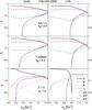 |
Fig. 2 Same as Fig. 1, but with the Dyson-Schwinger model for the quark phase. |
| In the text | |
|
Fig. 3 Pressure vs. baryon density for the same stellar configurations as in Fig. 1, and obtained with the MIT (left panels) and the DSM (right panels) quark models. |
| In the text | |
|
Fig. 4 Gravitational mass vs. central baryon density for different stellar configurations and EOS. |
| In the text | |
Current usage metrics show cumulative count of Article Views (full-text article views including HTML views, PDF and ePub downloads, according to the available data) and Abstracts Views on Vision4Press platform.
Data correspond to usage on the plateform after 2015. The current usage metrics is available 48-96 hours after online publication and is updated daily on week days.
Initial download of the metrics may take a while.