| Issue |
A&A
Volume 551, March 2013
|
|
|---|---|---|
| Article Number | A122 | |
| Number of page(s) | 8 | |
| Section | Cosmology (including clusters of galaxies) | |
| DOI | https://doi.org/10.1051/0004-6361/201220615 | |
| Published online | 05 March 2013 | |
New cosmological constraints on the variation of fundamental constants: the fine structure constant and the Higgs vacuum expectation value
1 Facultad de Ciencias Astronómicas y Geofísicas, Universidad Nacional de La Plata, Paseo del Bosque, 1900 La Plata, Argentina
e-mail: This email address is being protected from spambots. You need JavaScript enabled to view it.
2 Department of Physics, University of La Plata c.c. 67, 1900 La Plata, Argentina
Received: 23 October 2012
Accepted: 5 January 2013
Abstract
Aims. We study the time variation of the fine structure constant, α, and the Higgs vacuum expectation value v, during the Big Bang nucleosynthesis (BBN).
Methods. We computed primordial abundances of light nuclei produced during the BBN stage by including resonances in the leading reaction rates which reduce the primordial abundance of beryllium. We performed this calculation considering that α and v may vary during the BBN. Using observable data on deuterium, 4He, and 7Li, we set constraints on the variation of the fundamental constants.
Results. Results indicate a null variation of α and v, while the best-fit value for the baryon-to-photon ratio agrees well with the WMAP value.
Conclusions. We found that the variation of α is null within 3σ, the variation of v is null within 6σ, and the preferred value of the baryon-to-photon ratio is in good agreement, within 3σ, with the value extracted using the WMAP data. We improve the fits respect to previous works.
Key words: primordial nucleosynthesis / cosmology: miscellaneous / cosmological parameters
© ESO, 2013
1. Introduction
The attempt to unify all fundamental interactions resulted in the development of several theories such as string-derived field theories (Damour & Polyakov 1994; Wu & Wang 1986; Maeda 1988; Barr & Mohapatra 1988; Damour et al. 2002a,b), related brane-world theories (Youm 2001a,b; Palma et al. 2003; Brax et al. 2003) and Kaluza-Klein theories (Gleiser & Taylor 1985; Overduin & Wesson 1997; Kaluza 1921; Klein 1926; Weinberg 1983). These multidimensional theories allow fundamental constants to vary over cosmological timescales.
The experimental search on the variation of α and the Higgs vacuum expectation value v can be grouped into local and astronomical methods. The local methods include geophysical analyses of samples from the natural reactor in Oklo (Damour & Dyson 1996; Fujii et al. 2000), meteorites (Olive et al. 2004), and laboratory measurements of rates of atomics clocks (Bize et al. 2003; Fischer et al. 2004; Peik et al. 2004; Prestage et al. 1995; Sortais et al. 2000; Marion et al. 2003). The astronomical methods consist on the spectroscopic analysis of high-redshift quasar-absorption systems. Some of these astronomical observations suggest a possible variation of the fine structure constant and of the electron-to-proton mass ratio (Webb et al. 1999, 2001; Murphy et al. 2001a,b, 2003; Ivanchik et al. 2003, 2005; Reinhold et al. 2006; Tzanavaris et al. 2007; Levshakov et al. 2002b; Potekhin et al. 1998). However, another analysis of similar astronomical data gives a null variation of the fine structure constant (Martínez Fiorenzano et al. 2003; Quast et al. 2004; Bahcall et al. 2004; Srianand et al. 2004; King et al. 2008; Thompson et al. 2009; Malec et al. 2010).
Concerning the spatial variation of the fine structure constant, Webb et al. (2011) have analyzed the VLT (Very Large Telescope) data and reported that α increases at high redshift. However, the Keck telescope data show that the value of the fine structure constant is lower at high redshift. These contradictory results may indicate the presence of undetected systematic effects, or the need of a dipole model to explain for the variation of the fine structure constant. Note that both Keck and VLT data give the same direction and magnitude of the gradient of α. King et al. (2012) have re-analyzed the VLT and Keck Observatory data and found a non-null spatial variation of α, and that the dipole model is preferred over the monopole model. Berengut et al. (2011) have demonstrated that it is possible to set constraints on the spatial variation of the fine structure constant using Big Bang nucleosynthesis (BBN) primordial abundances, though the existing data on it do not support the dipole interpretation. A geophysical analysis to test the spatial variation of α was performed by Berengut & Flambaum (2012). These authors have concluded that the terrestrial limits do not contradict the reported observation, and have pointed out that the new measurements of primordial abundances, in different directions, could lead to the determination of the spatial variation of the fine structure constant during BBN.
The primordial production of light nuclei occurs during the first three minutes of the Universe, in a process called BBN. The formalism that explains this complex process has only one free parameter, the baryon density (or the baryon-to-photon ratio, these two quantities are related by a constant). This parameter can be determined by two different and independent methods. The first one is the comparison of the theoretical primordial abundances of deuterium, 4He, and 7Li with the observational data. The other method consists of analysing of the cosmic microwave background (CMB) data (Spergel et al. 2007; Larson et al. 2011). The theoretical abundances obtained by using the value of the baryon density provided by WMAP are consistent with the observed abundances of deuterium and 4He, but not with the lithium data. This so-called cosmological Li-problem was analyzed extensively in the literature. Richard et al. (2005) have suggested that a better understanding of the turbulent transport in the radiative zones of the stars is needed for a reliable estimation of the primordial abundance of 7Li. Others authors have suggested the existence of a stellar lithium depletion (this depletion depends on the mass of the star) (Meléndez et al. 2010; Lind et al. 2010). Some authors have analyzed the nuclear aspect of this problem (Broggini et al. 2013; Kirsebom & Davids 2011; Cyburt & Pospelov 2012). Including resonances in the nuclear reactions may reduce the abundance of lithium through depletion of the production of beryllium (Civitarese & Mosquera 2012). Several authors have studied the variation of the fundamental constants during the BBN. The dependence of the primordial abundances on the fine structure constant was evaluated by Bergström et al. (1999) and by Nollett & Lopez (2002). The effects of the variation of fundamental constants during BBN in the context of the dilaton superstring theory was analyzed by Campbell & Olive (1995) and by Ichikawa & Kawasaki (2002, 2004). The dependence of the primordial abundances as a function of the Planck mass, the fine structure constant, the Higgs vacuum expectation value, the electron mass, the nucleon decay time, the deuterium binding energy, and the neutron-proton mass difference was studied by Müller et al. (2004). Cyburt et al. (2005) have studied the variation of the fine structure constant and the variation of Newton’s GN. Coc et al. (2007) have set constraints on the variation in the neutron lifetime and the neutron-proton mass difference. Mosquera et al. (2008) have studied the variation of the fine structure constant in the early Universe and set constraints on the free parameters of the Bekenstein model (Bekenstein 1982), and in Scóccola et al. (2008) the variation of v in the early Universe (BBN and CMB) has been studied. In Mosquera & Civitarese (2011) and Landau et al. (2008) the variation of α and v during BBN have been studied without assuming any theoretical model for the variations.
If the fine structure constant can acquire any value during BBN, the light nuclear masses the variation of light nuclear masses, mx, can be written as  , where P is a constant on the order of 10-4, the neutron-proton mass difference
  ), the initial amount of neutrons and protons (
 ), the weak decay rates (through its dependence on the neutron to proton mass difference) and several reaction rates involved in BBN would change (Landau et al. 2006, 2008; Scóccola et al. 2008).
If the Higgs vacuum expectation value acquires a value during BBN different from the present one while the QCD coupling ΛQCD remains fixed, several quantities such as the electron mass, the deuterium binding energy, the Fermi constant (which is proportional to v-2 and affects the neutron to proton decay rates), the neutron-proton mass difference  ), and the mass of light nuclei would change with respect to their standard value (Dixit & Sher 1988; Christiansen et al. 1991; Yoo & Scherrer 2003). The effect of the variation of the electron mass is translated, in the calculations, into a variation of the sum of the electron and positron energy densities, the sum of the electron and positron pressures, and the difference of the electron and positron number densities (the change in these quantities affects the expansion rate, as is seen from Friedmann’s equation), the n ↔ p reaction rates, and the weak decay rates of heavy nuclei. If the neutron-proton mass difference varies with time, the initial amount of neutrons and protons, the n ↔ p, and the Q-values of several reactions (e.g. 3He(n, p)3H, 7Be(n, p)7Li) would be different than their present values. The variation of the light nuclei masses affects the Q-values and the reverse coefficient of the reactions that involve neutrons (Flambaum & Wiringa 2007).
In particular, the deuterium binding energy, ϵD, plays an important role during the BBN process. If the deuterium binding energy is modified, the initial value of the abundance of deuterium and the Q-value of reactions like d(γ, n)p, will be modified as well.
The dependence of the deuterium binding energy on the Higgs vacuum expectation value is model-dependent (Flambaum & Wiringa 2007). In the literature, this dependence was analyzed and the results have been applied to set constraints on the possible variation of the deuterium binding energy over cosmological timescales (Dmitriev et al. 2004; Flambaum & Shuryak 2002, 2003; Dmitriev & Flambaum 2003; Berengut et al. 2010). Yoo & Scherrer (2003) have used the lineal relationship between the deuterium binding energy and the Higgs vacuum expectation value obtained by Beane & Savage (2003); Epelbaum et al. (2003). In Mosquera & Civitarese (2010) and Civitarese et al. (2010) we have performed a detailed analysis of the lineal dependence of ϵD with v using different effective nucleon-nucleon potentials and set constraints on the variation of v.
In this work, we analyze the variation of the fine structure constant and the variation of the Higgs vacuum expectation value for a cosmological timescale (from the BBN until the present). We include isolated resonances in the calculation of the primordial abundances. We perform the calculation for three different cases: i) considering a resonance in the reaction 7Be + d → 4He + 4He + p; ii) including a resonance in the reaction 7Be + 4He → γ + 11C; and iii) considering both channels simultaneously. The parameters of the resonances were extracted from Broggini et al. (2013). Regarding the dependence of the deuterium binding energy upon the Higgs vacuum expectation value, we use the results obtained by Mosquera & Civitarese (2010) and Civitarese et al. (2010), that is, we have computed the primordial abundances for each one of the dependencies that are derived from the four different nucleon-nucleon effective potentials. Following Berengut et al. (2010) we assume that ΛQCD is constant, that is, we express all dimensions in units of ΛQCD and therefore, throughout, the relative variation  represents
  , where
  is a dimensionless parameter.
This work is organized as follows. In Sect. 2 we present the elements that are needed to compute the primordial abundances with a variation of the fundamental constants. In Sect. 3 we calculate the primordial abundances and obtain constraints on the variation of the fundamental constants for each case. The conclusions are presented in Sect. 4.
2. Formalism
We have modified the code developed by Kawano (1988, 1992) to include the variation of α and v in the fundamental quantities related to them. For details see Landau et al. (2006, 2008); Scóccola et al. (2008) and Mosquera & Civitarese (2011).
In Table 1 we present the values of the constant of proportionality, k, which relates the variation of ϵD and of v (1)obtained by Mosquera & Civitarese (2010) and Civitarese et al. (2010). In the previous equation we denote
 , and δv = vBBN − v, the subindex BBN indicates the value of the constant at primordial nucleosynthesis.
The decay rates for the chain of nuclear reactions involved in the calculations have been modified to account for isolated resonances in the participant nuclear spectra. We assume a Breit-Wigner formula for the description of the cross section for an isolated resonance (Fowler et al. 1975)  (2)where Γi is the partial width for the decay of the resonant state, Γ is the sum over all partial widths,
  , gr = 2Jr + 1 is the spin degeneracy, Jr the spin of the resonant state and Er is the resonance energy in the center of momentum system. The average cross section ⟨ σv ⟩ is written
  (3)where
  . The parameters of the resonances
  were extracted from Broggini et al. (2013).
3. Bounds from BBN
The starting point of the present study is the calculation of the light nuclei abundances. With them one can perform an statistical analysis  using observational data to obtain the best-fit parameters. Although the data of WMAP are able to constrain the baryon density, there exist still some degeneracies between the model parameters, namely the baryon density, the dark matter density, the ratio of the comoving sound horizon at decoupling to the angular diameter distance to the surface of last scattering, the reionization optical depth, the scalar spectral index, and the amplitude of the density fluctuations. For this reason, we have computed light nuclei abundances and performed the statistical analysis using observational data to obtain the best fit of α, the Higgs vacuum expectation value, and the baryon to photon ratio for the following cases:
-
i)
variation of α and keeping ηB fixed at the WMAP value,
 (Spergel et al. 2007; Larson et al. 2011);
 -
ii)
variation of α and ηB;
-
iii)
variation of v and
 ;
; -
iv)
variation of v and ηB;
-
v)
variation of α, v and
; -
vi)
variation of α, v and ηB.
The values for the observational abundance of deuterium considered in the present work, were presented in Ivanchik et al. (2010), Burles & Tytler (1998a,b), Crighton et al. (2004), Kirkman et al. (2003), Levshakov et al. (2002a), O’Meara et al. (2006, 2001), and Pettini et al. (2008).
We used the data from Izotov et al. (2006), Izotov & Thuan (2004), Thuan & Izotov (2002, 1998), Izotov et al. (1997, 1994), and Peimbert et al. (2007) for the primordial abundance of 4He.
Finally, the observational data for 7Li were extracted from Boesgaard et al. (2005), Molaro et al. (1997), Bonifacio & Molaro (1997), Bonifacio et al. (2002, 2007), Hosford et al. (2009), Ryan et al. (2000), Asplund et al. (2006), Sbordone et al. (2010), Meléndez et al. (2010), and Monaco et al. (2012).
To check the consistency of the data, we performed the analysis of Beringer et al. (2012) for the data set considered in the present work. We increased the standard deviation by a factor ΘD = 2.34 for the deuterium data and Θ7 = 1.41 for the data of lithium.
3.1. Variation of α with
For this case we computed the primordial abundances of the light elements considering that only the fine structure constant varies. The baryon-to-photon ratio remains constant at the WMAP value.
Best-fit values for  .
.
In Table 2 we present the results of  for the minimization of the χ2 test. There is a good fit when we considered that only one of the reactions has a resonance. For these two cases, the variation of the fine structure constant is null within 3σ (three standard deviations). When two resonances, one in each reaction rate, are treated, the fit is still good and the variation of α is null within 3σ.
3.2. Variation of α with a variable ηB
We computed the primordial abundances of the light elements allowing the variation of the fine structure constant and the baryon-to-photon ratio. We considered the three reactions mentioned above to include isolated resonances.
Best-fit values for and ηB.
The results are presented in Table 3. Clearly a good fit is achieved when only one of the reactions has a resonance. For these cases the variation of the fine structure constant is null within 2σ and the value of the baryon-to-photon ratio agrees well with the value obtained by the WMAP team within 3σ (Larson et al. 2011). The third row of Table 3 shows that the variation of α is null within 3σ and the value of ηB agrees well with the value  , but the fit is not as good as the previous ones.
In Figs. 1 to 3 we show the confidence contour plots and one-dimensional likelihood for each case. The results are quite similar, but if we incorporate two isolated resonances the contour plot allows a wider range of variation of α and of the value of ηB.
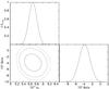 |
Fig. 1 Likelihood contours plots for ηB and |
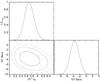 |
Fig. 2 Likelihood contours plots for ηB and |
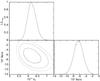 |
Fig. 3 Likelihood contour plots for ηB and |
From the present results it is clear that including the resonances improves the fit, and the best-fit value for is consistent with zero while the best-fit value of ηB perfectly agrees with the WMAP value within 3σ.
3.3. Variation of v with
We computed the primordial abundances of the light elements considering that only the Higgs vacuum expectation value during the BBN might be different than the present value. The baryon-to-photon ratio remains constant at the WMAP value.
In Table 4 we present the results for the different values of k and the different reaction rates with a new isolated resonance.
Best-fit values for  .
.
If we include the isolated resonances only in one reaction at a time, the fit is good. The variation of the Higgs vacuum expectation value for these cases is consistent with a null variation within 3σ. When both resonances are treated simultaneously, the fit becomes poorer than before and, once again, the variation of v is null within 3σ.
3.4. Variation of v allowing ηB to vary
The results for the best-fit values for and ηB during the BBN are presented in Table 5. The fit is good when we considered that each of the reactions has a resonance. If we incorporate the two isolated resonances simultaneously, the fit becomes poorer than the one including only one resonance at a time. For all the cases, the variation of the Higgs vacuum expectation value is null within 3σ and the value of the baryon-to-photon ratio agrees well with the value obtained by WMAP within 3σ.
Best-fit values for and ηB.
In Figs. 4 to 6 we present the confidence contour plots and one-dimensional likelihood for each case. As seen in the figures, the results considering two isolated resonances simultaneously allow for a wider range of variation of the value of ηB.
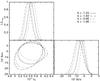 |
Fig. 4 3σ likelihood contour plots for ηB and |
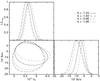 |
Fig. 5 3σ likelihood contour plots for ηB and |
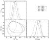 |
Fig. 6 3σ likelihood contour plots for ηB and |
Including the resonances improves the fit, and the best-fit value for is consistent with zero while the best-fit value of ηB perfectly agrees with the WMAP value within 3σ.
3.5. Variation of α and v with
We computed the primordial abundances of light nuclei considering the simultaneous variations of α and v for a constant value of the baryon-to-photon ratio. In Table 6 we present the results for different values of k and for the different reaction rates that include a new isolated resonance.
Best-fit values for and .
When we included the isolated resonance in only one channel, we found good fits, and the variation of the fine structure constant and the Higgs vacuum expectation value are null within 6σ (for the channel 7Be + d). When we included the isolated resonances in both reaction rates it will produce good fits, and the variation of the fine structure constant and the Higgs vacuum expectation value are null within 6σ for all values of k. In Figs. 7 to 9 we present the likelihood contour plots for the variation of α (in units of 103) and the variation of v (in units of 103) for all values of k used in the analysis.
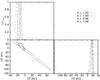 |
Fig. 7 3σ likelihood contour plots for |

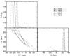 |
Fig. 8 3σ likelihood contour plots for |
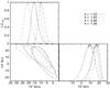 |
Fig. 9 3σ likelihood contour plots for |
Including the new resonances improves the fit, and the best-fit value for the variation of α and v is consistent with zero if the isolated resonances are included in the reactions.
3.6. Variation of α and v allowing ηB to vary
We computed the primordial abundances of light nuclei considering that α, v and ηB may vary with time. In Table 7 we present the results for the χ2-test.
Best-fit values for , and ηB.
Including an isolated resonance in only one reaction leads to good fits, and the variation of the fine structure constant and the Higgs vacuum expectation value are null within 2σ for all values of k. The value for the baryon-to-photon ratio agrees well with the value extracted using the WMAP data (Larson et al. 2011) within 1σ. When the isolated resonances are considered in both reaction rates, the statistical analysis yields good fits (although they are poorer than for the previous cases), and the variation of the fine structure constant and the Higgs vacuum expectation value are null within 4σ for all values of k. The value for the baryon-to-photon ratio agrees well with the WMAP value. In Figs. 10 to 12 we present the likelihood contours plots for ηB (in units of 1010), the variation of α (in units of 103), and the variation of v (in units of 103) for all values of k used in the analysis.
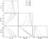 |
Fig. 10 3σ likelihood contours for ηB, |
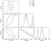 |
Fig. 11 3σ likelihood contour plots for ηB, |
Thus, for this case including the nuclear resonances improves the fit, the best-fit value for the variation of α and v is consistent with zero, and the value of ηB agrees well with the WAMP estimations (Larson et al. 2011).
3.7. Comparison with previous fits
To give an idea about the scope of the present results, in this section we compare them with the results obtained in previous fits, where the nuclear reaction was not modified by taking resonances into account.
3.7.1. Variation of α
In a previous work (Mosquera et al. 2008), it was shown that the inclusion of 7Li in the data set yields a poor χ2-value, and that either the variation of the fine structure constant was not null or the value of ηB disagreed with the WMAP data.
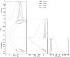 |
Fig. 12 3σ likelihood contour plots for ηB, |
3.7.2. Variation of v
In Scóccola et al. (2008), it was shown that either the variation of v was not null or the value of ηB disagreed with the WMAP data, and the χ2-test leads to not a good fit.
In Civitarese et al. (2010), we found that the variation of the Higgs vacuum expectation value was not null within 6σ, but the value of ηB agreed with the WMAP data.
3.7.3. Variation of α and v
In Landau et al. (2008) it was shown that the statistical analysis leads to a non-null variation of both fundamental constants within 6σ, and the value of ηB is not consistent with the estimations of WMAP within 3σ.
In a previous work (Mosquera & Civitarese 2011) it was found that the variation of the fine structure constant was null within 2σ, the variation of the Higgs vacuum expectation value was not null within 6σ, and the value of the baryon-to-photon ratio agreed well with the WMAP estimations.
4. Conclusion
We have analyzed the effects of including isolated resonances in some of the BBN reactions on the variation of the fine structure constant and the variation of the Higgs vacuum expectation value. We found that, in presence of resonances, the variation of α is null within 3σ. However, if the resonances are simultaneously included in all reactions, the fit is poorer than the previous one. The same features emerge if the baryon-to-photon ratio is taken as a free parameter adjusted by the observable data. In this case, the variation of α is null within 2σ and the value of ηB agrees well with the value provided by WMAP within 3σ. The contour plots obtained when both resonances are simultaneously included show a wider range for the value of the variation of the fine structure constant and the baryon-to-photon ratio than the ones obtained by taking the resonances separately.
The variation of v is null within 3σ for all cases. We also analyzed the case where the baryon-to-photon ratio is a free parameter to adjust using the observable data. In this case we found that the variation of v is null within 3σ and the value of ηB agrees well with the value provided by the WMAP team within 3σ. For all the dependencies of the deuterium binding energy on v the results are quite similar. Finally, we compared the different cases and found that if the isolated resonances are present in both reactions 7Be + d → 4He + 4He + p and 7Be + 4He → γ + 11C, the contour plots show a wider range for the allowed value of the baryon-to-photon ratio than those with only one resonance.
We found that the joint variation of α and v is null, and for the case of variable ηB we found that both the variation of α and the variation of v are null, and that the value of ηB agrees well with the value provided by WMAP.
As mentioned in Sect. 3.7, the present values are, in general, better than previously reported.
Acknowledgments
This work has been partially supported by the National Research Council (CONICET) of Argentina (PIP 0740) and by the ANPCyT (Argentina). The authors are members of the Scientific Research Career of the CONICET.
References
- Asplund, M., Lambert, D. L., Nissen, P. E., et al. 2006, ApJ, 644, 229 [NASA ADS] [CrossRef] [Google Scholar]
- Bahcall, J. N., Steinhardt, C. L., & Schlegel, D. 2004, ApJ, 600, 520 [NASA ADS] [CrossRef] [Google Scholar]
- Barr, S. M., & Mohapatra, P. K. 1988, Phys. Rev. D, 38, 3011 [NASA ADS] [CrossRef] [Google Scholar]
- Beane, S. R., & Savage, M. J. 2003, Nucl. Phys. A, 713, 148 [NASA ADS] [CrossRef] [Google Scholar]
- Bekenstein, J. D. 1982, Phys. Rev. D, 25, 1527 [NASA ADS] [CrossRef] [MathSciNet] [Google Scholar]
- Berengut, J. C., & Flambuam, V. V. 2012, Europhys. Lett., 97, 20006 [Google Scholar]
- Berengut, J. C., Flambaum, V. V., & Dmitriev, V. F. 2010, Phys. Lett. B, 683, 114 [NASA ADS] [CrossRef] [Google Scholar]
- Berengut, J. C., Flambaum, V. V., King, J. A., Curran, S. J., & Webb, J. K. 2011, Phys. Rev. D, 83, 123506 [NASA ADS] [CrossRef] [Google Scholar]
- Bergström, L., Iguri, S., & Rubinstein, H. 1999, Phys. Rev. D, 60, 45005 [Google Scholar]
- Beringer, J., Flambaum, V. V., King, J. A., et al. 2012 (Particle Data Group) Phys. Rev. D, 86, 010001 [Google Scholar]
- Bize, S., Diddams, S. A., Tanaka, U., et al. 2003, Phys. Rev. Lett., 90, 150802 [NASA ADS] [CrossRef] [PubMed] [Google Scholar]
- Boesgaard, A. M., Novicki, M. C., & Stephens, A. 2005, in From Lithium to Uranium: Elemental Tracers of Early Cosmic Evolution, eds. V. Hill, P. François, & F. Primas, IAU Symp., 228, 29 [Google Scholar]
- Bonifacio, P., & Molaro, P. 1997, MNRAS, 285, 847 [NASA ADS] [CrossRef] [Google Scholar]
- Bonifacio, P., Pasquini, L., Spite, F., et al. 2002, ApJ, 390, 91 [Google Scholar]
- Bonifacio, P., Molaro, P., Sivarani, T., et al. 2007, A&A, 462, 851 [NASA ADS] [CrossRef] [EDP Sciences] [Google Scholar]
- Brax, P., van de Bruck, C., Davis, A. C., & Rhodes, C. S. 2003, Astrophys. Space Sci., 283, 627 [Google Scholar]
- Broggini, C., Canton, L., Fiorentini, G., & Villante, F. L. 2013, JCAP, 06, 030 [NASA ADS] [Google Scholar]
- Burles, S., & Tytler, D. 1998a, ApJ, 507, 732 [NASA ADS] [CrossRef] [Google Scholar]
- Burles, S., & Tytler, D. 1998b, ApJ, 499, 699 [Google Scholar]
- Campbell, B. A., & Olive, K. A. 1995, Phys. Lett. B, 345, 429 [NASA ADS] [CrossRef] [Google Scholar]
- Christiansen, H. R., Epele, L. N., Fanchiotti, H., & García Canal, C. A. 1991, Phys. Lett. B, 267, 164 [NASA ADS] [CrossRef] [Google Scholar]
- Civitarese, O., & Mosquera, M. E. 2012, Nucl. Phys. A, 898, 1 [Google Scholar]
- Civitarese, O., Moliné, M. A., & Mosquera, M. E. 2010, Nucl. Phys. A, 846, 157 [NASA ADS] [CrossRef] [Google Scholar]
- Coc, A., Nunes, N. J., Olive, K. A., et al. 2007, Phys. Rev. D, 76, 023511 [NASA ADS] [CrossRef] [Google Scholar]
- Crighton, N. H. M., Webb, J. K., Ortiz-Gil, A., & Fernández-Soto, A. 2004, MNRAS, 355, 1042 [NASA ADS] [CrossRef] [Google Scholar]
- Cyburt, R. H., Fields, B. D., Olive, K. A., & Skillman, E. 2005, Astropart. Phys., 23, 313 [NASA ADS] [CrossRef] [Google Scholar]
- Cyburt, R. H., & Pospelov, M. 2012, Int. J. Mod. Phys. E, 21, 50004 [Google Scholar]
- Damour, T., & Polyakov, A. M. 1994, Nucl. Phys. B, 95, 10347 [Google Scholar]
- Damour, T., & Dyson, F. 1996, Nucl. Phys. B, 480, 37 [NASA ADS] [CrossRef] [MathSciNet] [Google Scholar]
- Damour, T., Piazza, F., & Veneziano, G. 2002a, Phys. Rev. Lett., 89, 081601 [Google Scholar]
- Damour, T., Piazza, F., & Veneziano, G. 2002b, Phys. Rev. D, 66, 046007 [NASA ADS] [CrossRef] [MathSciNet] [Google Scholar]
- Dixit, V. V., & Sher, M. 1988, Phys. Rev. D, 37, 1097 [NASA ADS] [CrossRef] [Google Scholar]
- Dmitriev, V. F., & Flambaum, V. V. 2003, Phys. Rev. D, 67, 063513 [NASA ADS] [CrossRef] [Google Scholar]
- Dmitriev, V. F., Flambaum, V. V., & Webb, J. K. 2004, Phys. Rev. D, 69, 063506 [NASA ADS] [CrossRef] [Google Scholar]
- Epelbaum, E., Meißner, U., & Glöckle, W. 2003, Nucl. Phys. A, 714, 535 [NASA ADS] [CrossRef] [Google Scholar]
- Fischer, M., Kolachevsky, N., Zimmermann, M., et al. 2004, Phys. Rev. Lett., 92, 230802 [NASA ADS] [CrossRef] [PubMed] [Google Scholar]
- Flambaum, V. V., & Shuryak, E. V. 2002, Phys. Rev. D, 65, 103503 [NASA ADS] [CrossRef] [Google Scholar]
- Flambaum, V. V., & Shuryak, E. V. 2003, Phys. Rev. D, 67, 083507 [NASA ADS] [CrossRef] [Google Scholar]
- Flambaum, V. V., & Wiringa, R. B. 2007, Phys. Rev. C, 76, 054002 [NASA ADS] [CrossRef] [Google Scholar]
- Fowler, W. A., Caughlan, G. R., & Zimmerman, B. A. 1975, ARA&A, 13, 69 [Google Scholar]
- Fujii, Y., Iwamoto, A., Fukahori, T., et al. 2000, Nucl. Phys. B, 573, 377 [NASA ADS] [CrossRef] [Google Scholar]
- Gleiser, M., & Taylor, J. G. 1985, Phys. Rev. D, 31, 1904 [NASA ADS] [CrossRef] [Google Scholar]
- Hosford, A., Ryan, S. G., García Pérez, A. E., et al. 2009, A&A, 493, 601 [NASA ADS] [CrossRef] [EDP Sciences] [Google Scholar]
- Ichikawa, K., & Kawasaki, M. 2002, Phys. Rev. D, 65, 123511 [NASA ADS] [CrossRef] [Google Scholar]
- Ichikawa, K., & Kawasaki, M. 2004, Phys. Rev. D, 69, 123506 [NASA ADS] [CrossRef] [Google Scholar]
- Ivanchik, A., Petitjean, P., Rodriguez, E., & Varshalovich, D. 2003, Astrophys. Space Sci., 283, 583 [NASA ADS] [CrossRef] [Google Scholar]
- Ivanchik, A., Petitjean, P., Varshalovich, D., et al. 2005, A&A, 440, 45 [NASA ADS] [CrossRef] [EDP Sciences] [Google Scholar]
- Ivanchik, A. V., Petitjean, P., Balashev, S. A., et al. 2010, MNRAS, 404, 1583 [NASA ADS] [Google Scholar]
- Izotov, Y. I., & Thuan, T. X. 2004, ApJ, 602, 200 [CrossRef] [Google Scholar]
- Izotov, Y. I., Thuan, T. X., & Lipovetsky, V. A. 1994, ApJ, 435, 647 [NASA ADS] [CrossRef] [Google Scholar]
- Izotov, Y. I., Thuan, T. X., & Lipovetsky, V. A. 1997, ApJS, 108, 1 [NASA ADS] [CrossRef] [Google Scholar]
- Izotov, Y. I., Schaerer, D., Blecha, A., et al. 2006, A&A, 459, 71 [NASA ADS] [CrossRef] [EDP Sciences] [Google Scholar]
- Kaluza, T. 1921, Sitzungber. Preuss. Akad. Wiss.K, 1, 966 [Google Scholar]
- Kawano, L. 1988, fERMILAB-PUB-88-034-A [Google Scholar]
- Kawano, L. 1992, fERMILAB-PUB-92-004-A [Google Scholar]
- King, J. A., Webb, J. K., Murphy, M. T., & Carswell, R. F. 2008, Phys. Rev. Lett., 101, 251304 [NASA ADS] [CrossRef] [PubMed] [Google Scholar]
- King, J. A., Webb, J. K., Murphy, M. T., et al. 2012, MNRAS, 422, 3370 [NASA ADS] [CrossRef] [Google Scholar]
- Kirkman, D., Tytler, D., Suzuki, N., et al. 2003, ApJS, 149, 1 [NASA ADS] [CrossRef] [Google Scholar]
- Kirsebom, O. S., & Davids, B. 2011, Phys. Rev. C, 84, 058801 [NASA ADS] [CrossRef] [Google Scholar]
- Klein, O. 1926, Z. Phys., 37, 895 [Google Scholar]
- Landau, S. J., Mosquera, M. E., & Vucetich, H. 2006, ApJ, 637, 38 [NASA ADS] [CrossRef] [Google Scholar]
- Landau, S. J., Mosquera, M. E., Scóccola, C. G., & Vucetich, H. 2008, Phys. Rev. D, 78, 083527 [NASA ADS] [CrossRef] [Google Scholar]
- Larson, D., Dunkley, J., Hinshaw, G., et al. 2011, ApJS, 192, 16 [NASA ADS] [CrossRef] [Google Scholar]
- Levshakov, S. A., Dessauges-Zavadsky, M., D’Odorico, S., & Molaro, P. 2002a, ApJ, 565, 696 [NASA ADS] [CrossRef] [Google Scholar]
- Levshakov, S. A., Dessauges-Zavadsky, M., & D’Odorico, S. P. M. 2002b, MNRAS, 333, 373 [NASA ADS] [CrossRef] [Google Scholar]
- Lind, K., Primas, F., Charbonnel, C., et al. 2010, in IAU Symp. 268, eds. C. Charbonnel, M. Tosi, F. Primas, & C. Chiappini, 263 [Google Scholar]
- Müller, C. M., Schäfer, G., & Wetterich, C. 2004, Phys. Rev. D, 70, 083504 [NASA ADS] [CrossRef] [Google Scholar]
- Maeda, K. 1988, Mod. Phys. Lett. A, 31, 243 [Google Scholar]
- Malec, A. L., Buning, R., Murphy, M. T., et al. 2010, MNRAS, 403, 1541 [NASA ADS] [CrossRef] [Google Scholar]
- Marion, H., et al. 2003, Phys. Rev. Lett., 90, 150801 [NASA ADS] [CrossRef] [PubMed] [Google Scholar]
- Martínez Fiorenzano, A. F., Vladilo, G., & Bonifacio, P. 2003, Soc. Astron. It. Mem. Suppl., 3, 252 [NASA ADS] [Google Scholar]
- Meléndez, J., Casagrande, L., Ramírez, I., et al. 2010, A&A, 515, L3 [NASA ADS] [CrossRef] [EDP Sciences] [Google Scholar]
- Molaro, P., Bonifacio, P., & Pasquini, L. 1997, MNRAS, 292, L1 [NASA ADS] [CrossRef] [Google Scholar]
- Monaco, L., Villanova, S., Bonifacio, P., et al. 2012, A&A, 539, A157 [NASA ADS] [CrossRef] [EDP Sciences] [Google Scholar]
- Mosquera, M. E., & Civitarese, O. 2010, A&A, 520, A112 [NASA ADS] [CrossRef] [EDP Sciences] [Google Scholar]
- Mosquera, M. E., & Civitarese, O. 2011, A&A, 526, A109 [NASA ADS] [CrossRef] [EDP Sciences] [Google Scholar]
- Mosquera, M. E., Scóccola, C., Landau, S., & Vucetich, H. 2008, A&A, 478, 675 [NASA ADS] [CrossRef] [EDP Sciences] [Google Scholar]
- Murphy, M. T., Webb, J. K., Flambaum, V. V., et al. 2001a, MNRAS, 327, 1208 [NASA ADS] [CrossRef] [Google Scholar]
- Murphy, M. T., Webb, J. K., Flambaum, V. V., et al. 2001b, MNRAS, 327, 1237 [NASA ADS] [CrossRef] [Google Scholar]
- Murphy, M. T., Webb, J. K., & Flambaum, V. V. 2003, MNRAS, 345, 609 [Google Scholar]
- Nollett, K. M., & Lopez, R. E. 2002, Phys. Rev. D, 66, 063507 [NASA ADS] [CrossRef] [Google Scholar]
- Olive, K. A., Pospelov, M., Qian, Y. Z., et al. 2004, Phys. Rev. D, 69, 027701 [NASA ADS] [CrossRef] [Google Scholar]
- O’Meara, J. M., Tytler, D., Kirkman, D., et al. 2001, ApJ, 552, 718 [NASA ADS] [CrossRef] [Google Scholar]
- O’Meara, J. M., Burles, S., Prochaska, J. X., et al. 2006, ApJ, 649, L61 [NASA ADS] [CrossRef] [Google Scholar]
- Overduin, J. M., & Wesson, P. S. 1997, Phys. Rep., 283, 303 [NASA ADS] [CrossRef] [MathSciNet] [Google Scholar]
- Palma, G. A., Brax, P., Davis, A. C., & van de Bruck, C. 2003, Phys. Rev. D, 68, 123519 [NASA ADS] [CrossRef] [Google Scholar]
- Peik, E., Lipphardt, B., Schnatz, H., et al. 2004, Phys. Rev. Lett., 93, 170801 [NASA ADS] [CrossRef] [Google Scholar]
- Peimbert, M., Luridiana, V., & Peimbert, A. 2007, ApJ, 666, 636 [NASA ADS] [CrossRef] [Google Scholar]
- Pettini, M., Zych, B. J., Murphy, M. T., et al. 2008, MNRAS, 391, 1499 [NASA ADS] [CrossRef] [MathSciNet] [Google Scholar]
- Potekhin, A. Y., Ivanchik, A. V., Varshalovich, D. A., et al. 1998, ApJ, 505, 523 [NASA ADS] [CrossRef] [Google Scholar]
- Prestage, J. D., Tjoelker, R. L., & Maleki, L. 1995, Phys. Rev. Lett., 74, 3511 [NASA ADS] [CrossRef] [PubMed] [Google Scholar]
- Quast, R., Reimers, D., & Levshakov, S. A. 2004, A&A, 415, L7 [NASA ADS] [CrossRef] [EDP Sciences] [Google Scholar]
- Reinhold, E., et al. 2006, Phys. Rev. Lett., 96, 151101 [NASA ADS] [CrossRef] [Google Scholar]
- Richard, O., Michaud, G., & Richer, J. 2005, ApJ, 619, 538 [NASA ADS] [CrossRef] [Google Scholar]
- Ryan, S. G., Beers, T. C., Olive, K. A., et al. 2000, ApJ, 530, L57 [NASA ADS] [CrossRef] [PubMed] [Google Scholar]
- Sbordone, L., Bonifacio, P., Caffau, E., et al. 2010, A&A, 522, A26 [NASA ADS] [CrossRef] [EDP Sciences] [Google Scholar]
- Scóccola, C. G., Mosquera, M. E., Landau, S. J., & Vucetich, H. 2008, ApJ, 681, 737 [NASA ADS] [CrossRef] [Google Scholar]
- Sortais, Y., et al. 2000, Phys. Scr. T, 95, 50 [NASA ADS] [CrossRef] [Google Scholar]
- Spergel, D. N., Bean, R., Doré, O., et al. 2007, ApJS, 170, 377 [NASA ADS] [CrossRef] [Google Scholar]
- Srianand, R., Chand, H., Petitjean, P., & Aracil, B. 2004, Phys. Rev. Lett., 92, 121302 [NASA ADS] [CrossRef] [PubMed] [Google Scholar]
- Thompson, R. I., Bechtold, J., Black, J. H., et al. 2009, ApJ, 703, 1648 [NASA ADS] [CrossRef] [Google Scholar]
- Thuan, T. X., & Izotov, Y. I. 1998, Space Sci. Rev., 84, 83 [NASA ADS] [CrossRef] [Google Scholar]
- Thuan, T. X., & Izotov, Y. I. 2002, Space Sci. Rev., 100, 263 [NASA ADS] [CrossRef] [Google Scholar]
- Tzanavaris, P., Murphy, M. T., Webb, J. K., et al. 2007, MNRAS, 374, 634 [NASA ADS] [CrossRef] [Google Scholar]
- Webb, J. K., Murphy, M., Flambaum, V., et al. 2001, Phys. Rev. Lett., 87, 091301 [NASA ADS] [CrossRef] [PubMed] [Google Scholar]
- Webb, J. K., King, J. A., Murphy, M. T., et al. 2011, Phys. Rev. Lett., 107, 191101 [NASA ADS] [CrossRef] [Google Scholar]
- Webb, J. K., Flambaum, V. V., Churchill, C. W., et al. 1999, Phys. Rev. Lett., 82, 884 [Google Scholar]
- Weinberg, S. 1983, Phys. Lett. B, 125, 265 [NASA ADS] [CrossRef] [Google Scholar]
- Wu, Y., & Wang, Z. 1986, Phys. Rev. Lett., 57, 1978 [NASA ADS] [CrossRef] [PubMed] [Google Scholar]
- Yoo, J. J., & Scherrer, R. J. 2003, Phys. Rev. D, 67, 043517 [NASA ADS] [CrossRef] [Google Scholar]
- Youm, D. 2001a, Phys. Rev. D, 63, 125011 [NASA ADS] [CrossRef] [Google Scholar]
- Youm, D. 2001b, Phys. Rev. D, 64, 085011 [NASA ADS] [CrossRef] [Google Scholar]
All Tables
All Figures
|
Fig. 1 Likelihood contours plots for ηB and |
| In the text | |
|
Fig. 2 Likelihood contours plots for ηB and |
| In the text | |
|
Fig. 3 Likelihood contour plots for ηB and |
| In the text | |
|
Fig. 4 3σ likelihood contour plots for ηB and |
| In the text | |
|
Fig. 5 3σ likelihood contour plots for ηB and |
| In the text | |
|
Fig. 6 3σ likelihood contour plots for ηB and |
| In the text | |
|
Fig. 7 3σ likelihood contour plots for |
| In the text | |
|
Fig. 8 3σ likelihood contour plots for |
| In the text | |
|
Fig. 9 3σ likelihood contour plots for |
| In the text | |
|
Fig. 10 3σ likelihood contours for ηB, |
| In the text | |
|
Fig. 11 3σ likelihood contour plots for ηB, |
| In the text | |
|
Fig. 12 3σ likelihood contour plots for ηB, |
| In the text | |
Current usage metrics show cumulative count of Article Views (full-text article views including HTML views, PDF and ePub downloads, according to the available data) and Abstracts Views on Vision4Press platform.
Data correspond to usage on the plateform after 2015. The current usage metrics is available 48-96 hours after online publication and is updated daily on week days.
Initial download of the metrics may take a while.