| Issue |
A&A
Volume 551, March 2013
|
|
|---|---|---|
| Article Number | A102 | |
| Number of page(s) | 6 | |
| Section | Planets and planetary systems | |
| DOI | https://doi.org/10.1051/0004-6361/201220490 | |
| Published online | 01 March 2013 | |
Do Slivan states exist in the Flora family?
II. Fingerprints of the Yarkovsky and YORP effects⋆
Astronomical Observatory Institute, Faculty of Physics, Adam Mickiewicz
University,
Słoneczna 36,
60-286
Poznań,
Poland
e-mail: This email address is being protected from spambots. You need JavaScript enabled to view it.
Received: 3 October 2012
Accepted: 15 January 2013
Abstract
Context. It is known that the Yarkovsky effect moves small astroids to larger/smaller semimajor axes depending on their prograde/retrograde spins. The YORP effect influences asteroid spin periods and spin axis orientations so that they evolve in time. The alignment of the spin vectors and correlations of the spin rates, now known as Slivan states and observed among members of the Koronis family, are interpreted in terms of the YORP effect and spin-orbit resonances. Splitting asteroid families into prograde and retrograde groups has recently been proposed as a result of the Yarkovsky effect. Prograde and retrograde asteroids drift in different directions, and this has never been observed directly.
Aims. The influence of the Yarkovsky and YORP effects should be observable among objects in asteroid families, especially in the Flora family, which lies close to the Sun and consists of many small objects.
Methods. The Flora family asteroids were modelled using the lightcurve inversion technique. As a result the orientation of spin vectors, shapes, and sidereal periods of rotation were obtained.
Results. Results of modelling of the Flora family asteroids show the family splitting into prograde and retrograde groups as a result of the Yarkovsky effect. The observed ratio between prograde and retrograde asteroids is 2.6. The positions of spin vectors, as well as their similar latitudes suggest, that the Slivan states are observed among the Flora family asteroids.
Conclusions. The influence of the Yarkovsky and YORP effect is clearly visible in the Flora family. The location of the Flora family close to the ν6 resonance explains the lack of retrograde objects and confirms the excess of retrograde rotators among NEAs and their origin from the ν6. The Slivan states that I searched seem to be present among prograde rotators in this family even though they were not expected.
Key words: minor planets, asteroids: general / techniques: photometric
Photometric data are only available at the CDS via anonymous ftp to cdsarc.u-strasbg.fr(130.79.128.5) or via http://cdsarc.u-strasbg.fr/viz-bin/qcat?J/A+A/551/A102
© ESO, 2013
1. Introduction
The rotational properties of asteroids can be determined from analysing their lightcurves. However, parameters like the position of rotation axis, the shape model, and the sense of rotation require many observations in various observing circumstances. Such parameters are available for about 250 objects, but only 170 have reasonably reliable determinations, all listed in the present databases (Kryszczynska et al. 2007; Durech et al. 2010). In general, the ecliptic latitude and the longitude are the two angles describing the spin vector orientation.
From a theoretical point of view, the spin properties of asteroids should depend mainly on their collisional evolution, with only the largest ones retaining any memory of the original properties (Davies et al. 1989). Collisional disruption of the homogenous parent body should result in random distribution of spin vectors in the resulting fragments. Recently some additional processes have been proposed capable of affecting asteroids orbital and spin properties: the Yarkovsky (Vokrouhlicky 1998, 1999; Vokrouhlicky & Farinella 1998; Bottke et al. 2001; Morbidelli & Vokrouhlicky 2003; Spitale & Greenberg 2001) and the YORP effects (Rubincam 2000). It is known that the Yarkovsky moves objects to larger/smaller semimajor axes depending on their prograde/retrograde spins. The YORP effect influences the asteroids spin periods and also primarily moves the spin axes away from the ecliptic plane. In this case, the Yarkovsky drift becomes more effective.
The influence of the Yarkovsky effect on particular asteroids was directly detected for the first time by radar observations of 6489 Golevka (Chesley et al. 2003) The influence of the YORP effect was observed among members of the Koronis family (Slivan 2002; 2009). These asteroids have correlated rotation rates and aligned spin vectors. The prograde rotators have clustered spin period values (from 7.5 h to 9.5 h) and spin axis orientation (obliquities from 42° to 50°). Retrograde rotators have rotation periods shorter than 5 h or longer than 13 h, and the spin axis orientation is almost perpendicular to their orbits, as well as to the ecliptic plane (obliquities larger than 154°).
The unexpected nonrandom orientations of spin axes and correlation of spin rates were explained by a model of the YORP effect and spin-orbit resonances by Vokrouhlicky et al. (2003). They found that the prograde rotator’s period and obliquity evolve due to YORP torques, and eventually the asteroid is captured by the s6 spin-orbit’s secular resonance between the precession rate of asteroid’s spin axis and Saturn’s longitude of node. Objects trapped in the resonance were said by Vokrouhlicky et al. (2003) to be in a Slivan state. The YORP effect also modifies the spin states of the Koronis family retrograde asteroids. It spins up or spins down the asteroid rotation and forces the position of the spin axis to become perpendicular to the orbit (obliquity close to 180°). Vokrouhlicky et al. (2003) predicts that outer belt asteroids might be found in Slivan states, but that in the inner asteroid belt, the spin-axis evolution would be too chaotic with large oscillations rather than evolving to 55°. The importance of a careful comparison between numerical results and observations was also pointed out.
The interesting behaviour of the members of the Koronis family was an inspiration to study another asteroid family, namely the Flora family. This family was chosen because of its close distance to the Sun and very effective secular resonance with Saturn ν6. Its location allows for observations of small objects that have diameters ≤ 30 km and are potentially sensitive to the influence of both the Yarkovsky and YORP effects. It can be expected that the influence of the Yarkovsky and YORP effects should also be observable among the members of the Flora family. The results of the ten-year long photometric campaign of the Flora family asteroids were described in the first paper of the series (Kryszczynska et al. 2012, called hereafter Paper I). In this paper the results of modelling the Flora family asteroids are presented.
2. Modelling the Flora family asteroids
The objects considered in this study were identified as members of the Flora family by two different methods, hierarchical clustering (HCM) and wavelet analysis (WAM), of classifying asteroids into families (Bendjoya & Zappala 2002). The classification was performed on a dataset of more than 12 000 asteroids’ proper elements. The resulting families had about 600 members and 75% of their objects in common. The recent family identification was based on a dataset of almost 300 000 asteroids’ proper elements. Using HCM Nesvorny (2010) obtained more than 10 000 objects belonging to the Flora family. Dynamical methods, however, are not sensitive to the asteroids’ surface parameters and may classify some interlopers in the family. Identification of them requires additional observations of their physical properties.
Sixteen new models of the objects identified as Flora family members (by HCM and/or WAM) were obtained using the lightcurve inversion technique (Kaasalainen & Torppa 2001; Kaasalainen et al. 2001). All new lightcurves used for modelling are available in Paper I. Some older publicly available data was also used in modelling. Newly determined models will be available at ISAM (Interactive Service for Asteroids Models, Marciniak et al. 2012).
Summary of information on the Flora family asteroids.
3. Results
Models presented in this section are based on asteroid lightcurves alone. In several cases they are compared with the Hanus et al. (2011) results, which are usually based on only a few lightcurves and sparse data or sparse data. Comparison of the results shows that several good quality lightcurves combined with sparse data improve the final solution for the sidereal period of rotation and position of the spin axis.
3.1. Comments on individual asteroids
291 Alice
A preliminary model of Alice was based on only six lightcurves (Kryszczynska at al. 1996) so no sense of rotation and sidereal period was determined. The old spin vector coordinates are surprisingly consistent with the new determination based on 19 lightcurves. The model of Alice based on nine lightcurves and sparse data (Hanus et al. 2011) gives a similar position for the spin vector.
367 Amicitia
The model of Amicitia obtained by Hanus et al. (2011) is based on only two lightcurves (which do not cover the whole period of rotation) and sparse data. The latitude of pole is about 20 degrees lower, and the sidereal period is slightly longer than the values presented in this paper. The new model is based on seventeen lightcurves.
700 Auravictrix
A preliminary model of Auravictrix presented by Shevchenko et al. (2009) was based on only four lightcurves. They did not determine the sidereal period and the sense of rotation. The model presented here is based on nineteen lightcurves observed from 1977 to 2011.
770 Bali
The model of Bali presented in this paper is close to the one derived by Hanus et al. (2011), based on two lightcurves and sparse data.
800 Kressmannia
The model of Kressmannia obtained by Hanus et al. (2011) is based on eight lightcurves and sparse data. The latitude of pole is about 20 degrees lower and the sidereal period is slightly longer than the values presented in this paper. The new model is based on twenty-seven lightcurves.
825 Tanina
The model presented here, based on twenty-five lightcurves, is similar to the one obtained by Hanus et al. (2011), and it is based on two lightcurves and sparse data.
915 Cosette
The model of Cosette presented in this paper is very similar to the model obtained by Hanus et al. (2011) based on only a single lightcurve and sparse data.
937 Bethgea, 1675 Simonida, 2017 Wesson, 281 Lucretia, 352 Gisela
The models presented in this paper are the first ones obtained for these objects. All of them are based on a long period of observations, more than 20 years, and large collection of lightcurves.
1088 Mitaka
The model presented here is close to the one derived by Hanus et al. (2011), based on a single lightcurve and sparse data.
1188 Gothlandia, 1219 Britta
The determinations presented here are the first complete models for these asteroids.
2156 Kate
The model of Kate obtained by Hanus et al. (2011) is based on four lightcurves and sparse data. The sidereal period is 0.000078 h longer than the one presented here, however the position of the spin vector is close to the determination presented in this paper.
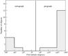 |
Fig. 1 Distribution of the latitude for the poles of 18 Flora family asteroids. The zones referred to in the abscissa are defined with the same conventions as in Pravec et al. (2002), representing approximately equal surfaces on the λ,β sphere; region 1 means retrograde, from −90° to −45°, 2 means −45° to −25°, 3 means −25° to −8°, 4 means −8° to 8° (prograde) and so on. The histogram looks exactly the same if we put the spin vector north pole obliquity in the abscissa. |
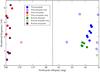 |
Fig. 2 Relation between spin vector obliquity and rotation frequency of the Flora (blue and red dots) and the Koronis (green and brown squares) family members. Dots and squares of different pattern represent stray objects, that does not seem to fit to the grouping The abscissa are defined with the same convention as in Slivan (2002). The error bars for the rotational frequency lie within the marked symbols and are several degrees for the spin vector obliquity (see Table 1). |
Three additional, already known spin vectors for 951 Gaspra (all determinations collected at the Poznan Observatory website, Kryszczynska et al. 2007), 1514 Ricouxa, and 1682 Karel (Hanus et al. 2011) were added to this study, however the last two objects are of unknown taxonomic type and therefore they may be interlopers. The model of 1682 Karel based on only sparse data (Hanus et al. 2011) should be checked with the help of lightcurves. The high albedo of 1682 Karel of 0.531 taken from AcuA (Asteroid Catalog Using AKARI/IRC mid-infrared survey, Usui et al. 2011) suggests that this object might be an interloper in the Flora family. The main body of a younger subcluster in the Flora family, 1270 Datura was excluded (Vokrouhlicky et al. 2009). Both 810 Atossa and 2156 Kate, identified by one of the clustering method and different than S taxonomic type, which are probable interlopers in the Flora family, were also excluded, because asteroid families in the main belt are rather homogenous taxonomically (Cellino et al. 2002; Mothe-Diniz et al. 2005).
The results are summarized in Table 1. Columns represent the asteroid number and name, the ecliptic longitude λp(°) and latitude βp(°) of the asteroid pole (usually two solutions different by 180°), the spin vector obliguity ϵ(°) (the angle beetween the orbit pole and the spin pole), the sidereal period of rotation Psid(h), the frequency of rotation f in rotations per day, the period when lightcurves were collected, the number of lightcurves used in modelling N, the family identification method: HCM – hierarchical clustering, WAM – wavelet analysis method, the taxonomic type. Taxonomic types were taken from the Planetary Data System (Neese 2010), the SDSS-based Asteroid Taxonomy (Hasselman et al. 2011), and Alvarez-Candal et al. (2006). The details can be found in Paper I.
Figure 1 presents the distribution of the spin vectors ecliptic latitudes for the 18 Flora family asteroids listed in Table 1. The histogram looks exactly the same if we put the spin vector north pole obliquity in the abscissa. Figure 1 shows that most of the poles are far from the ecliptic plane, as well as from the orbit plane, which is consitent with a long-term evolution due to the YORP effect. Moreover, there is a group of eight objects (291, 367, 700, 770, 800, 825, 915, 1675) of almost equal obliquity of their spin vectors from 31° to 42° and similar periods from 4.3 to 6.9 h, which are supposed to be in the Slivan states. (The adopted obliquity is a mean value of two very close solutions available in Table 1.) The obliquities are close to those found among the Koronis family members from 41° to 52° (Slivan 2002, 2009).
The comparison of obliquities and rotation frequencies of the Koronis and the Flora asteroids is shown in Fig. 2 which is drawn with the same convention as in Slivan (2002). Stray objects, which does not seem to fit to the grouping, still (at least for some cases) might be consistent with YORP explanation for the distribution of its spin vectors. It is worth noticing that eight additional preliminary models of the Koronis family asteroids were presented by Slivan et al. (2008). Five of them merge the retrograde group, but three appear to be stray objects.
Most of the retrograde objects in the Flora family have obliquities greater than 150° and periods shorter than about 5.5 h, which is consistent with the long-term evolution due to the YORP effect. Figure 2 shows similar behaviour to the retrograde objects of the Flora and the Koronis families.
The excess of prograde rotators versus retrograde is also clearly visible. The observed ratio between prograde and retrograde asteroids is NP/NR = 2.6. This ratio was never considered in asteroid family modelling. A selection effect might explain this difference, but there is no obvious reason that the family-forming asteroid disruption should create more prograde than retrograde rotators. However, there is a reason that retrograde objects from the Flora family are favoured to become NEAs or Mars crossers.
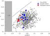 |
Fig. 3 Positions of prograde (blue dots) and retrograde (red dots) asteroids in proper-element space: orbit semimajor axis a [AU] versus eccentricity e. The grey path shows the position of ν6 resonance (which depends on orbit inclination). The Mars-crossing line for q = 1.83 AU is shown. |
Figure 3 presents positions of prograde and retrograde asteroids in proper-element space: the orbit semimajor axis a (AU) versus eccentricity e, and the position of ν6 resonace (which depends on orbit inclination). Figure 4 presents the same asteroids on the semimajor axis a (AU) versus sine of inclination i plane and the position of the centre of the ν6 resonance. In both figures retrograde objects are closer to ν6, their orbital semimajor axes are smaller, while prograde objects are at larger semimajor axes. This splitting is consistent with the Yarkovsky drift. The one prograde S-type object 800 Kressmannia is observed at a lower semimajor axis than the rest of the prograde asteroids (Figs. 3–5). This object could have been ejected with very high velocity during the collision of the parent body, and despite the influence of the Yarkovsky effect, there was not enough time for it to reach the prograde group. It is also possible that this asteroid is simply an interloper and not a family member at all, or that its spin axis was dramatically altered in a later collisional event.
The excess of prograde asteroids is caused by the Yarkovsky drift, which moves retrograde bodies into the ν6 resonance region. Missing objects were probably ejected by ν6 to the inner parts of the Solar System and became NEAs or Mars crossers.
The Yarkovsky-driven splitting between prograde and retrorade rotators is also visible in Fig. 5, which presents absolute magnitude H (mag) as a function of proper semimajor axis a (AU). Positions of 123 Flora family objects with known spin periods of rotation, reported in Paper I are also presented (from 8 Flora up to the number 4150 Starr, all smaller than 30 km).
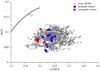 |
Fig. 4 Positions of prograde (blue dots) and retrograde (red dots) asteroids in proper-element space: orbit semimajor axis a [AU] versus sine of inclination. The brown line shows the position of the centre of the ν6 resonace. |
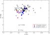 |
Fig. 5 Absolute magnitude H (mag) as a function of semimajor axis a (AU) for Flora family asteroids. The grey circles represent 123 Flora family objects with known spin periods of rotation (from 8 Flora up to number 4150 Starr) smaller than 30 km. The positions of retrograde are shown as red dots, and prograde as blue dots. The largest members of the family – 8 Flora and 43 Ariadne – are also presented. |
4. Discussion and conclusions
Vokrouhlicky et al. (2003) investigated whether asteroids in regions other than near Koronis may be trapped in the Slivan state. Their preliminary results predict that Slivan states may be found for low inclination asteroids in the outer main belt. A more complex spin vector evolutionary path was found for test objects in the other regions of the main belt, partly connected with the overlapping spin-orbit resonaces. They also suggest that it was important to carefully compare numerical results and observations.
The studied spin properties of the Flora family asteroids confirm the expected influence of the Yarkovsky and YORP effects. The Slivan states I searched seem to be present among prograde rotators in this family even though they were not expected. Three asteroids in this group, 291 Alice, 367 Amicita, and 825 Tanina with the lowest orbital inclinations, are probably trapped in the Slivan state (Vokrouhlicky, pres. comm.). The spin states of the other objects in the group require more detailed studies.
The excess of prograde rotators is connected with the influence of the very effective secular resonance with Saturn ν6, which lies at the inner edge of the family, as well as at the edge of the main belt, and it can be reached only by retrograde object owing to the Yarkovsky effect. Bottke at al. (2000, 2002) suggest that ≈ 37% of all NEAs (with absolute magnitude H < 18 mag) came from the ν6 resonance, with the rest coming from a variety of different source regions, among them major mean motion resonances, such as J3:1, J2:1 and others. All of the escape channels for NEAs except ν6 can be reached by both prograde and retrograde asteroids. For this reason the theoretical ratio between NEAs with retrograde/prograde spins is 2 ± 0.2 (Bottke et al. 2000, 2002). The present datasets of NEAs’ known spin vectors give a surprisingly good fit (La Spina et al. 2004; Paolicchi & Kryszczynska 2012). The lack of retrograde asteroids in the Flora family is consistent with the excess of retrograde rotators among NEAs and their origin from ν6 resonance. The injection of asteroids into inner regions of the Solar System is strongly influenced by the Yarkovsky effect and ν6 resonace. Some of the population of asteroids lost to the resonance are currently observed as NEAs, and some of them reside on transitional orbits between the main belt and the Sun.
Acknowledgments
I would like to thank the referee Kevin Walsh for his helpful remarks and suggestions for improving the paper. I would like to thank David Vokrouhlicky for taking the time to discuss the results of my modelling. This work was supported by the Narodowe Centrum Nauki Grant N N203 382136.
References
- Alvarez-Candal, A., Duffard, R., Lazzaro, D., & Mitchenko, T. 2006, A&A, 459, 969 [NASA ADS] [CrossRef] [EDP Sciences] [Google Scholar]
- Bendjoya, P., & Zappala, V. 2002, In Asteroids III, eds. W. F. Bottke, et al. (Arizona Univ. Press), 613 [Google Scholar]
- Bottke, W. F., Jedicke, R., Morbidelli, A., et al. 2000, Science, 288, 2190 [NASA ADS] [CrossRef] [PubMed] [Google Scholar]
- Bottke, W. F., Vokrouhlicky, D., Broz, M., Nesvorny, D., & Morbidelli, A. 2001, Science, 294, 1693 [NASA ADS] [CrossRef] [PubMed] [Google Scholar]
- Bottke, W. F., Morbidelli, A., Jedicke, R., et al. 2002, Icarus, 156, 399 [NASA ADS] [CrossRef] [Google Scholar]
- Chesley, S. R., Ostro, S. J., Vokrouhlický, D., et al. 2003, Science, 302, 1739 [NASA ADS] [CrossRef] [Google Scholar]
- Cellino, A., Buss, S. J., Doressoundiram, A., & Lazzaro, D. 2002, in Asteroids III, eds. W. F. Bottke, A. Cellino, P. Paolicchi, & R. P. Binzel (Tucson: Univ. Arizona Press), 633 [Google Scholar]
- Davis, D. R., Weidenschilling, S. J., Farinella, P., Paolicchi, P., & Binzel, R. P. 1989, in Asteroids II, eds. R. P. Binzel, et al. (Tucson: Arizona Univ. Press), 805 [Google Scholar]
- Durech, J., Sidorin, V., & Kaasalainen, M. 2010, A&A, 513, A46 [NASA ADS] [CrossRef] [EDP Sciences] [Google Scholar]
- Hanus, J., Ďeurech, J., Brože, M., et al. 2011, A&A, 530, A134 [NASA ADS] [CrossRef] [EDP Sciences] [Google Scholar]
- Hasselmann, P. H., Carvano, J. M., & Lazzaro, D. 2011, SDSS-based Asteroid Taxonomy V1.0, EAR-A-I0035-5-SDSSTAX-V1.0, NASA Planetary Data System [Google Scholar]
- Kaasalainen, M., & Torppa, J. 2001, Icarus, 153, 24 [NASA ADS] [CrossRef] [Google Scholar]
- Kaasalainen, M., Torppa, J., & Muinonen, K. 2001, Icarus, 153, 37 [NASA ADS] [CrossRef] [Google Scholar]
- Kryszczynska, A., Colas, F., Berthier, J., et al. 1996, Icarus, 124, 134 [NASA ADS] [CrossRef] [Google Scholar]
- Kryszczynska, A., La Spina, A., Paolicchi, P., et al. 2007, Icarus, 192, 223 [NASA ADS] [CrossRef] [Google Scholar]
- Kryszczynska, A., Colas, F., Polińska, M., et al. 2012, A&A, 546, A72 [NASA ADS] [CrossRef] [EDP Sciences] [Google Scholar]
- La Spina, A., Paolicchi, P., Kryszczynska, A., & Pravec, P. 2004, Nature, 428, 400 [NASA ADS] [CrossRef] [PubMed] [Google Scholar]
- Marciniak, A., Bartczak, P., Santana-Ros, T., et al. 2012, A&A, 545, A131 [NASA ADS] [CrossRef] [EDP Sciences] [Google Scholar]
- Morbidelli, A., & Vokrouhlicky, D. 2003, Icarus, 163, 120 [NASA ADS] [CrossRef] [Google Scholar]
- Mothe-Diniz, T., Roig, F., & Carvano, J. M. 2005, Icarus, 174, 54 [NASA ADS] [CrossRef] [Google Scholar]
- Neese, C., ed. 2010, Asteroid Taxonomy V6.0, EAR-A-5-DDR-TAXONOMY-V6.0, NASA Planetary Data System [Google Scholar]
- Nesvorny, D. 2010, Asteroid Families V1.0, EAR-A-VARGBDET-5-NESVORNYFAM-V1.0, NASA Planetary Data System [Google Scholar]
- Paolicchi, P., & Kryszczynska, A. 2012, P&SS, 73, 70 [Google Scholar]
- Pravec, P., Harris, A. W., & Michalowski, T. 2002, in Asteroids III, eds. W. F. Bottke, A. Cellino, P. Paolicchi, & R. P. Binzel (Univ. Arizona Press, Tucson), 113 [Google Scholar]
- Rubincam, D. P. 2000, Icarus, 148, 2 [NASA ADS] [CrossRef] [Google Scholar]
- Shevchenko, V. G., Tungalag, N., Chiorny, V. G., et al. 2009, P&SS, 57, 1514 [NASA ADS] [CrossRef] [Google Scholar]
- Spitale, J., & Greenberg, R. 2001, Icarus, 149, 222 [NASA ADS] [CrossRef] [Google Scholar]
- Slivan, S. M. 2002, Nature, 419, 49 [Google Scholar]
- Slivan, S. M., Binzel, R. P., Kaasalainen, M., et al. 2008, BAAS, 40, 425 [NASA ADS] [Google Scholar]
- Slivan, S. M., Binzel, R. P., Kaasalainen, M., et al. 2009, Icarus, 200, 514 [NASA ADS] [CrossRef] [Google Scholar]
- Usui, F., Kuroda, D., Muller, T. G., et al. 2011, PASJ, 63, 1117 [NASA ADS] [CrossRef] [Google Scholar]
- Vokrouhlicky, D. 1998, A&A, 335, 1093 [NASA ADS] [Google Scholar]
- Vokrouhlicky, D. 1999, A&A, 344, 362 [NASA ADS] [Google Scholar]
- Vokrouhlicky, D., & Farinella, P. 1998, AJ, 116, 2032 [Google Scholar]
- Vokrouhlicky, D., Durech, J., Michalowski, T., et al. 2009, A&A, 507, 495 [NASA ADS] [CrossRef] [EDP Sciences] [Google Scholar]
- Vokrouhlicky, D., Nesvorny, D., & Bottke, W. F. 2003, Nature, 425, 147 [NASA ADS] [CrossRef] [PubMed] [Google Scholar]
All Tables
All Figures
|
Fig. 1 Distribution of the latitude for the poles of 18 Flora family asteroids. The zones referred to in the abscissa are defined with the same conventions as in Pravec et al. (2002), representing approximately equal surfaces on the λ,β sphere; region 1 means retrograde, from −90° to −45°, 2 means −45° to −25°, 3 means −25° to −8°, 4 means −8° to 8° (prograde) and so on. The histogram looks exactly the same if we put the spin vector north pole obliquity in the abscissa. |
| In the text | |
|
Fig. 2 Relation between spin vector obliquity and rotation frequency of the Flora (blue and red dots) and the Koronis (green and brown squares) family members. Dots and squares of different pattern represent stray objects, that does not seem to fit to the grouping The abscissa are defined with the same convention as in Slivan (2002). The error bars for the rotational frequency lie within the marked symbols and are several degrees for the spin vector obliquity (see Table 1). |
| In the text | |
|
Fig. 3 Positions of prograde (blue dots) and retrograde (red dots) asteroids in proper-element space: orbit semimajor axis a [AU] versus eccentricity e. The grey path shows the position of ν6 resonance (which depends on orbit inclination). The Mars-crossing line for q = 1.83 AU is shown. |
| In the text | |
|
Fig. 4 Positions of prograde (blue dots) and retrograde (red dots) asteroids in proper-element space: orbit semimajor axis a [AU] versus sine of inclination. The brown line shows the position of the centre of the ν6 resonace. |
| In the text | |
|
Fig. 5 Absolute magnitude H (mag) as a function of semimajor axis a (AU) for Flora family asteroids. The grey circles represent 123 Flora family objects with known spin periods of rotation (from 8 Flora up to number 4150 Starr) smaller than 30 km. The positions of retrograde are shown as red dots, and prograde as blue dots. The largest members of the family – 8 Flora and 43 Ariadne – are also presented. |
| In the text | |
Current usage metrics show cumulative count of Article Views (full-text article views including HTML views, PDF and ePub downloads, according to the available data) and Abstracts Views on Vision4Press platform.
Data correspond to usage on the plateform after 2015. The current usage metrics is available 48-96 hours after online publication and is updated daily on week days.
Initial download of the metrics may take a while.