| Issue |
A&A
Volume 551, March 2013
|
|
|---|---|---|
| Article Number | A127 | |
| Number of page(s) | 11 | |
| Section | Interstellar and circumstellar matter | |
| DOI | https://doi.org/10.1051/0004-6361/201220276 | |
| Published online | 05 March 2013 | |
Numerical simulations of composite supernova remnants for small σ pulsar wind nebulae
1
Centre for Space Research, School of Physics, North-West
University,
2520
Potchefstroom,
South Africa
e-mail:
This email address is being protected from spambots. You need JavaScript enabled to view it.
2
CNRS, Université Paris 7, Denis Diderot, 75005
Paris,
France
Received:
22
August
2012
Accepted:
30
January
2013
Abstract
Context. Composite supernova remnants consist of a pulsar wind nebula located inside a shell-type remnant. The presence of a shell has implications on the evolution of the nebula, although the converse is generally not true.
Aims. The purpose of this paper is two-fold. The first aim is to determine the effect of the pulsar’s initial luminosity and spin-down rate, the supernova ejecta mass, and density of the interstellar medium on the evolution of a spherically-symmetric, composite supernova remnant expanding into a homogeneous medium. The second aim is to investigate the evolution of the magnetic field in the pulsar wind nebula when the the composite remnant expands into a non-uniform interstellar medium.
Methods. The Euler conservation equations for inviscid flow, together with the magnetohydrodynamic induction law in the kinematic limit, are solved numerically for a number of scenarios where the ratio of magnetic to particle energy is σ < 0.01. The simulations in the first part of the paper is solved in a one-dimensional configuration. In the second part of the paper, the effect of an inhomogeneous medium on the evolution is studied using a two-dimensional, axisymmetric configuration.
Results. It is found that the initial spin-down luminosity and density of the interstellar medium has the largest influence on the evolution of the pulsar wind nebula. The spin-down time-scale of the pulsar only becomes important when this value is smaller than the time needed for the reverse shock of the shell remnant to reach the outer boundary of the nebula. For a remnant evolving in a non-uniform medium, the magnetic field along the boundary of the nebula will evolve to a value that is larger than the magnetic field in the interior. If the inhomogeneity of the interstellar medium is enhanced, while the spin-down luminosity is decreased, it is further found that a magnetic “cloud” is formed in a region that is spatially separated from the position of the pulsar.
Key words: supernovae: general / magnetohydrodynamics (MHD) / ISM: supernova remnants / hydrodynamics
© ESO, 2013
1. Introduction
It is well-known that a supernova explosion causes a shock wave that travels through the interstellar medium (ISM), creating a shell-like supernova remnant (SNR) that can be visible from radio to TeV energies (e.g. Woltjer 1972; Aharonian et al. 2006). This shock wave is not a single entity, but consists of three distinct parts: a forward shock that propagates into the ISM, a reverse shock, and a contact discontinuity separating the two shocks (e.g. Truelove & McKee 1999). Initially the reverse shock expands outwards along with the forward shock, but will eventually start to propagate into the interior of the SNR when a sufficient amount of ambient matter has been swept-up by the forward shock (McKee 1974).
The rate at which the SNR expands depends on a number of factors, including the mass of the stellar material ejected during the supernova explosion, Mej, the amount of kinetic energy transferred to the ejecta, typically of the order Eej ~ 1051 erg, and the density of the interstellar medium ρism (e.g. Dwarkadas & Chevalier 1998; Truelove & McKee 1999; Tang & Wang 2005; Ferreira & De Jager 2008). Additionally, the adiabatic index, γ, can also influence the evolution of a SNR due to the non-linear interaction of accelerated cosmic rays on SNR shocks (e.g. Decourchelle et al. 2000; Ellison et al. 2004). For a comprehensive discussion of the evolution of SNRs, the papers of e.g. Sedov (1959), Woltjer (1972), Chevalier (1977), and McKee & Truelove (1995) can be consulted.
A possible by-product of a core-collapse supernova (e.g. Woosley & Janka 2005) is a pulsar, which in turn can lead to the presence of a second type of supernova remnant, commonly referred to as a pulsar wind nebula (PWN). As the name suggests, the nebula is formed by a wind that originates from the pulsar and flows into the surrounding medium. It is believed that this wind consists of relativistic leptons (electrons and positrons), and possibly a hadronic component (e.g. Horns et al. 2006), with the pulsar’s magnetic field frozen into the plasma. When the ram pressure of the wind is equal to the particle and magnetic pressure of the surrounding medium (created in earlier epochs of the pulsar wind), a termination shock will form (Rees & Gunn 1974) where the particles are accelerated (e.g. Kennel & Coroniti 1984). Downstream of the termination shock the accelerated leptons interact with the frozen-in magnetic field to produce synchrotron radiation ranging from radio to X-ray energies. Additionally, the leptons can also inverse Compton scatter ambient photons to GeV and TeV gamma-ray energies. The source of the ambient photons is typically the Cosmic Microwave Background Radiation, although infra-red radiation from dust, starlight, and even the synchrotron photons can also contribute. The synchrotron and inverse Compton emission create a luminous nebula around the pulsar, with the pulsar continuously supplying energy to the PWN. For a review of PWNe, the papers of Gaensler & Slane (2006), Kargaltsev & Pavlov (2008) and De Jager & Djannati-Ataï (2009) can be consulted.
An interesting subclass of SNRs are the systems consisting of a pulsar wind nebula located within a shell component. Although the dynamics of the shell remnant is not influenced by the evolution of the PWN, the presence of a shell remnant can have a notable influence on the evolution of the PWN. This one-sided interaction can be ascribed to the difference in energy content of the two components, with the shell remnant having a significantly larger amount of energy (e.g. Reynolds & Chevalier 1984). Simulations show that the evolution of a PWN can be divided into a number of stages (e.g. Reynolds & Chevalier 1984; Van der Swaluw et al. 2004). In the initial stage the PWN expands supersonically into the SNR ejecta until the reverse shock reaches the boundary of the PWN. In the following stage the reverse shock compresses the PWN, with the interaction leading to the formation of a reflection wave that travels trough the PWN. Calculations predict that the second stage should start at ~103−104 yr after the initial explosion (e.g. Reynolds & Chevalier 1984; Van der Swaluw et al. 2004). The final stage is characterised by the subsonic expansion of the PWN into the ejecta heated by the reverse shock.
Pulsars are often born with large kick-velocities, possibly resulting from an asymmetric supernova explosion. The PWN is initially created at the centre of the SNR, but will be dragged along by the pulsar as it moves through the interior of the SNR (Van der Swaluw et al. 2004). This reduces the distance between the shell and the PWN in the direction that the pulsar moves, thereby decreasing the time needed for the reverse shock to reach the forward boundary of the PWN. For the opposite boundary, the reverse shock interaction time is correspondingly increased. The different reverse shock interaction times leads the formation of a cigar-shaped nebula with the pulsar located at the edge (Van der Swaluw et al. 2004). The PWN continues to expand, while a bow-shock eventually forms at the nebula’s edge closest to the pulsar when approximately two-thirds of the SNR radius has been traversed (Van der Swaluw et al. 2003).
Additionally, pulsars with a sufficiently large proper motion can break through the SNR shell and escape into the ISM, with the escape time for a 1000 km s-1 pulsar estimated to be around ~40 000 yr (Van der Swaluw et al. 2003). A study of the velocity distribution of radio pulsars found characteristics at 90 km s-1 and 500 km s-1 (Arzoumanian et al. 2002). It was further estimated that 15% of the pulsars have velocities greater than 1000 km s-1, and that only 10% of pulsars younger than 20 000 yr will be found outside the SNR (Arzoumanian et al. 2002).
Although the asymmetry observed in the morphology of PWNe can often be attributed to the large kick-velocities (e.g. Gaensler & Slane 2006), interaction of the forward shock with a non-homogeneous ISM can lead to a similar morphology (Blondin et al. 2001). It has been argued that the elongated morphology of (e.g.) Vela X and G09+0.1 is a result of the mentioned interaction, rather than a large proper motion of the pulsar (Blondin et al. 2001).
In a previous paper, Ferreira & De Jager (2008) calculated how the parameters Mej, Eej, ρism, and γ influence the evolution of a SNR, with a part of their study focusing on the evolution of the shell in a non-uniform ISM. In this work we extend their study by presenting hydrodynamic simulations of the evolution of a composite remnant containing a PWN for which the ratio of electromagnetic to particle energy is σ < 0.01. One aim of the paper is to investigate how the pulsar’s initial luminosity and spin-down time-scale, the mass of the supernova ejecta, and the density of the ISM influence the evolution of the PWN. This parameter study is done for a spherically-symmetric remnant expanding into a homogeneous ISM. The second aim of this paper is to illustrate the evolution of an axisymmetric PWN in a non-homogeneous ISM, with an emphasis on the evolution of the magnetic field.
The outline of the paper is as follows: Sect. 2 introduces the model that is used, with the spherically-symmetric, homogeneous ISM, results presented in Sect. 3. Section 4 motivates the use of the kinetic approach by illustrating that a more correct treatment of the magnetic field leads to similar results if σ < 0.01. The axisymmetric, inhomogeneous ISM results are presented in Sect. 5, while the final section of the paper deals with the summary and conclusions.
2. Model and parameters
SNR evolution in uniform and non-uniform media has been modelled extensively by e.g. Tenorio-Tagle et al. (1991), Borkowski et al. (1997), Jun &
Jones (1999), while simulations focusing on selected aspects regarding the
evolution of PWNe and composite remnants have been presented by e.g. Van der Swaluw et al. (2001), Blondin et
al. (2001), Bucciantini (2002), Bucciantini et al. (2003), Van der Swaluw (2003), Del Zanna et al.
(2004), Bucciantini et al. (2005), Chevalier (2005). Similar to many of these studies, the
present model is based on the well-known Euler equations for inviscid flow describing
respectively the balance of mass, momentum and energy 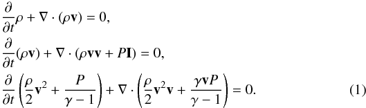 (1)Here
ρ is the density, v the velocity, and P the
pressure of the fluid. The evolution of the magnetic field, B, is calculated by
solving the induction equation
(1)Here
ρ is the density, v the velocity, and P the
pressure of the fluid. The evolution of the magnetic field, B, is calculated by
solving the induction equation 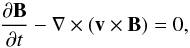 (2)in the kinematic limit
(Scherer & Ferreira 2005; Ferreira & Scherer 2006). In this approach, a
one-sided interaction between the fluid and B is assumed, with the effect of
B on the evolution of the flow neglected. This approach is sufficient when
the ratio of magnetic to particle energy is small, and will be further motivated in a later
section.
(2)in the kinematic limit
(Scherer & Ferreira 2005; Ferreira & Scherer 2006). In this approach, a
one-sided interaction between the fluid and B is assumed, with the effect of
B on the evolution of the flow neglected. This approach is sufficient when
the ratio of magnetic to particle energy is small, and will be further motivated in a later
section.
The Euler Eq. (1), are solved numerically using a hyperbolic scheme based on a wave propagation approach, as discussed in detail in LeVeque (2002) (see also Ferreira & De Jager 2008 for additional details), while the scheme presented by Trac & Pen (2003) is used for the induction Eq. (2). The model is solved in a spherical coordinate system with 0.01 ≤ r ≤ 25 pc and 0° ≤ θ ≤ 180°. For PWNe evolving in a homogeneous medium (Sect. 3), the complexity of the problem reduces to a one-dimensional, spherically-symmetric scenario, and the corresponding results are discussed in this context. For the simulations a 2400 × 25 grid is used for the homogeneous ISM, while the number of θ grid points is increased from 25 to 85 for the inhomogeneous ISM scenarios.
In solving the equations, any relativistic effects are neglected, whereas a more realistic
model should take into account that velocity of the particles between the pulsar and the PWN
termination shock is highly relativistic. However, since the post-shock flow must be
subsonic, i.e. v must be less than the sound speed in a relativistic plasma
( ),
smoothly decreasing towards the edge of the PWN, one expects that the fluid velocity in the
PWN should decrease from mildly relativistic to non-relativistic.
),
smoothly decreasing towards the edge of the PWN, one expects that the fluid velocity in the
PWN should decrease from mildly relativistic to non-relativistic.
A second possible limitation arises from considering a one-fluid scenario in which only a
single value for the adiabatic index, γ, is specified. A more correct model
would treat the stellar ejecta and PWN as two separate fluids, with
γej = 5/3 for the ejecta and
γpwn = 4/3 for the PWN. Van der Swaluw et al. (2001) showed that this limitation
can be compensated for in the one-fluid model by setting
γ = 5/3, while choosing the value for the mass
deposition rate at the inner boundary of the computational domain,
Ṁpwn, as  where
c is the speed of light. Using a two-fluid, one-dimensional, relativistic
magnetohydrodynamic (MHD) model, Bucciantini et al.
(2003) found that the size of the PWN is only ~10% smaller compared to one-fluid
simulations using γ = 5/3.
where
c is the speed of light. Using a two-fluid, one-dimensional, relativistic
magnetohydrodynamic (MHD) model, Bucciantini et al.
(2003) found that the size of the PWN is only ~10% smaller compared to one-fluid
simulations using γ = 5/3.
A further simplification in the present model is related to radiative losses being
neglected in the evolution of the SNR. The main emphasis of this study is on the interaction
of the PWN with the reverse shock of the shell, and the subsequent evolution of the PWN. The
only limitation is that the time needed for the reverse shock to propagate back towards the
PWN (e.g. Ferreira & De Jager 2008)
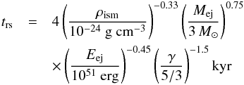 (3)must
be smaller than the time when radiative losses become important (Blondin et al. 1998)
(3)must
be smaller than the time when radiative losses become important (Blondin et al. 1998) 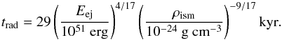 (4)As discussed in a
previous paragraph, the present model uses γ = 5/3,
together with the fiducial value Eej = 1051 erg. The
time-scales (3) and (4) are thus reduced to a function of the ejecta
mass and ISM density. For any permutation of the values Mej and
ρism chosen from the ranges
Mej = 4−16 M⊙ and
ρism = 10-25−10-23gcm-3,
one has
trs < trad.
(4)As discussed in a
previous paragraph, the present model uses γ = 5/3,
together with the fiducial value Eej = 1051 erg. The
time-scales (3) and (4) are thus reduced to a function of the ejecta
mass and ISM density. For any permutation of the values Mej and
ρism chosen from the ranges
Mej = 4−16 M⊙ and
ρism = 10-25−10-23gcm-3,
one has
trs < trad.
One shortcoming of the kinematic approach is that it does not reproduce the required PWN morphology in the initial evolutionary phase. Axisymmetric, two-dimensional MHD simulations, extending up to t = 1000 yr, have shown that the magnetic field in the PWN leads to an elongation of the nebula from a spherical to an elliptic-like shape, with a ratio of 1.3−1.5 between the semi-major and semi-minor axes (Van der Swaluw 2003). This non-spherical structure will induce time delays between the interaction of the reverse shock with the polar/equatorial regions of the PWN. A similar feature is predicted by the axisymmetric, two-dimensional, relativistic MHD simulations of Del Zanna et al. (2004). However, the latter authors found that the elongation increases to a maximum value at around t = 400 yr, before decreasing again. When the ratio of magnetic to particle energy is σ = 0.01, the elongation ratio decreases to a value that is less than 1.2 after t = 1000 yr. Since the simulations only extend up to t = 1000 yr, it may be possible that the elongation will reduce further. Additionally, Del Zanna et al. (2004) also found that the elongation ratio reaches unity after t = 1000 yr for the case σ = 0.003. Note that the simulations presented in this paper are specifically for scenarios where σ < 0.01.
It is unclear what role the asymmetric structure plays in the long-term evolution of the PWN since this has, to the authors’ knowledge, not been studied. It is heuristically argued that the effect would not be as pronounced as one would expect. When the reverse shock reaches the polar boundary, the nebula will be compressed in these regions and the thermal pressure increased. Due to the large sound speed in a PWN, the nebula will reach pressure equilibrium in a very short time. The larger pressure in the PWN will lead to an accelerated expansion in the regions where the reverse shock has not yet interacted with the PWN, specifically in the equatorial regions. This, in turn, reduces the time needed for the reverse shock to reach the equator of the PWN, leading to a more “symmetric” interaction between the PWN and reverse shock. Alternatively, it may also be argued that the evolution of the PWN is significantly more dependent on factors such as a large pulsar kick velocity or and inhomogeneous ISM.
Simulations have shown that the interaction of the reverse shock with the PWN leads to the formation of Raleigh-Taylor instabilities (e.g. Blondin et al. 2001; Van der Swaluw et al. 2004; Bucciantini et al. 2004a). Additionally, the same instabilities are expected to occur at the forward shock of young SNRs (e.g. Blondin et al. 2001). An initial test of the present numerical scheme found that these instabilities can be produced if a sufficiently fine computational grid is used. However, to avoid numerical dissipation, the grid has to be refined to such a degree that the code becomes extremely computationally intensive. Since the aim of the present paper is to simulate the large-scale evolution and structure of the PWN, any further investigation and discussion of these instabilities are neglected.
In the initial configuration of the system (e.g. Blondin
& Ellison 2001; Van der Swaluw et al.
2001; Bucciantini et al. 2003; Del Zanna et al. 2004) the SNR is spherical with a radius
Rej = 0.1 pc and a radially increasing velocity profile
 (5)with
 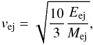 (6)while the density of the
ejecta is uniform in the interior of the SNR
(6)while the density of the
ejecta is uniform in the interior of the SNR 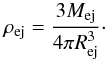 (7)Note that in the initial
condition the PWN is absent, with the particles injected by the pulsar only included after
the first time-step.
(7)Note that in the initial
condition the PWN is absent, with the particles injected by the pulsar only included after
the first time-step.
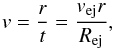
For the boundary conditions (e.g. Blondin & Ellison
2001; Van der Swaluw et al. 2001; Bucciantini et al. 2003; Del Zanna et al. 2004), the speed of the particles injected at the inner boundary
of the computational domain is equal to the speed of light, c, while the
density is calculated from the mass deposition rate (Van der
Swaluw 2003)  (8)where
  (9)is the spin-down luminosity
of the pulsar. The variable τ is known as the spin-down time scale, and is
defined by
(9)is the spin-down luminosity
of the pulsar. The variable τ is known as the spin-down time scale, and is
defined by  (10)with
L0 and P0 respectively the initial
luminosity and spin period, I the moment of inertia, and n
the pulsar braking index.
(10)with
L0 and P0 respectively the initial
luminosity and spin period, I the moment of inertia, and n
the pulsar braking index.
The magnetic field at the inner boundary is assumed to be purely azimuthal, in accordance
with theory (e.g. Rees & Gunn 1974) and
previous PWN models (e.g. Van der Swaluw 2003), while
an expression for the time evolution of the magnetic field strength,
B(t), at the inner boundary is derived as follows: the
spin-down luminosity, L(t), at any given position,
r, upstream of the pulsar wind termination shock can be written as (Kennel & Coroniti 1984)  (11)where σ is
the ratio of electromagnetic to particle energy. Equation (11) is effectively a statement of the conservation of energy, and is
valid for any value of σ. Since Eq. (11) should hold for all times, t, one may also state
that
(11)where σ is
the ratio of electromagnetic to particle energy. Equation (11) is effectively a statement of the conservation of energy, and is
valid for any value of σ. Since Eq. (11) should hold for all times, t, one may also state
that  (12)Inserting Eqs. (12) into (9) leads to the expression
  (13)To calculate the
time-dependence of B, the right-hand sides of Eqs. (11) and (13) are equated, while it is assumed that σ has no time
dependence at the inner boundary, leading to the result
(13)To calculate the
time-dependence of B, the right-hand sides of Eqs. (11) and (13) are equated, while it is assumed that σ has no time
dependence at the inner boundary, leading to the result  (14)In addition, the initial
value of the magnetic field at the inner boundary of the computational domain is normalised
to B0 = 1. This is possible since the magnetic field (in the
present) model does not influence the dynamics of the PWN.
(14)In addition, the initial
value of the magnetic field at the inner boundary of the computational domain is normalised
to B0 = 1. This is possible since the magnetic field (in the
present) model does not influence the dynamics of the PWN.
For the simulations, the initial luminosity ranges between L0 = 1037−1040 erg s-1, and the spin-down time-scale between τ = 500−5000 yr. Based on observations, e.g., Zhang et al. (2008); Fang & Zhang (2010); Tanaka & Takahara (2011) have derived similar L0 and τ values for a number of PWNe. Core-collapse supernovae (where pulsars are produced as a by-product) are expected to take place for stars with masses ≳8 M⊙ (e.g. Woosley & Janka 2005). As an example, a value of Mej ~ 11−15 M⊙ has been derived for SN 1987A (e.g. Shigeyama & Nomoto 1990). In the simulations the ejecta mass ranges between Mej = 8−12 M⊙. Furthermore, core-collapse supernovas occur in star forming regions (e.g. Woosley & Janka 2005) in the ISM with densities ranging from ρism = 10-26−10-23gcm-3 (e.g. Thornton et al. 1998), and a similar range chosen for the model. Lastly, the fiducial values Eej = 1051 erg and n = 3 are used for the simulations.
Van der Swaluw & Wu (2001) investigated the role of P0 on the evolution of a composite remnant, and concluded that if P0 ≤ 4 ms, the energy in the pulsar wind exceeds the total mechanical energy of the SNR, resulting in the SNR being blown away. This result is indirectly supported by the findings of Faucher-Giguère & Kaspi (2006). Using alternative means, these authors calculated P0 for a number of galactic pulsars, with P0 = 11 ms being the lowest value found. The values of L0 and τ, related through Eq. (10), must therefore be chosen in such a way as to not result in an unrealistic P0, with the definition of “realistic” being (loosely) defined as P0 ≳ 4 ms. Using the fiducial values I = 1045gcm2 and n = 3 for the moment of inertia and braking index of the pulsar, the smallest P0 value for the present simulations is found for the L0 = 1040 erg, τ = 5000 yr scenario, where P0 = 3.5 ms. Although this scenario is technically below the accepted limit, it is nevertheless included for the purpose of illustration.
3. Evolution of a PWN inside a spherically-symmetric SNR
In this section the effect of the parameters L0, τ, Mej, and ρism on the evolution of a spherically-symmetric PWN in a homogeneous ISM is investigated. In order to better compare the various scenarios, it is useful to define a basis set of parameters, chosen as L0 = 1039 erg s-1 for the initial luminosity, τ = 3000 yr for the spin-down time-scale, Mej = 12 M⊙ for the mass of the stellar ejecta, and ρism = 10-25 gcm-3 as the density of the ISM.
3.1. The outer boundary of the PWN
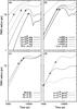 |
Fig. 1 Model solutions for the evolution of the outer boundary of a spherically-symmetric PWN in a homogeneous ISM. A basis parameter set is chosen as L0 = 1039 erg s-1, τ = 3000 yr, Mej = 12 M⊙, and ρism = 10-25 gcm-3, with the solution represented by a short-dashed line in panels a)–d). The other solutions were obtained by using the basis parameters, while varying the parameters listed in the legends of the figures. The ◇ symbol represents the time when the reverse shock reaches Rpwn. Also shown in panels a) and b) is the evolution of the forward shock of the SNR. |
Figure 1 shows the effect of the parameters on the evolution of the outer boundary of the nebula, Rpwn. The solutions were obtained with the basis values, only varying the appropriate variable as stated in the legends of the figures. The basis solution in the various panels of Fig. 1 is represented with a short-dashed line. Figures 1a–b also shows the evolution of the forward shock of the SNR. Since the forward shock is not dependent on the values of L0 and τ, the evolution is the same for all scenarios shown in these two panels. For Figs. 1c–d, the evolution of the forward shock is the same as that described in Ferreira & De Jager (2008). Before the interaction with the reverse shock (indicated by the ◇ symbols), the rate of expansion of the PWN can be described by a power-law function, Rpwn ∝ t1.1−1.3, similar to the prediction Rpwn ∝ t1.2 made by Reynolds & Chevalier (1984).
For the different L0 scenarios in Fig. 1a, a larger PWN is predicted when L0 is increased. This difference in PWN size can be attributed to the larger L0 scenarios having a faster expansion rate at the earliest times, t < 100 yr, with the expansion rate eventually evolving to Rpwn ∝ t1.2. Larger L0 values not only lead to a larger PWN, but also imply that more particles are injected into the PWN per time interval, thereby increasing the pressure in the PWN. For the L0 = 1040 erg s-1 scenario, the interaction with the reverse shock does not lead to a compression of the PWN, but only a slower (subsonic) expansion rate. For the L0 = 1037 erg s-1 scenario (where the PWN pressure is smaller), the reverse shock noticeably compresses the PWN, with the post-interaction expansion rate having an oscillatory nature.
At times t ≲ τ, the value of L0 is almost constant, and any variation in τ should not affect the evolution of Rpwn. This can be seen from the results in Fig. 1b where the evolution of Rpwn at times t ≲ 5000 yr is very similar for the various scenarios. The exception is the τ = 500 yr scenario where a smaller PWN is predicted. The largest influence of τ is seen after the interaction with the reverse shock. Since a smaller τ leads to a faster decrease in L(t), the PWN pressure should correspondingly decrease, leading to a larger compression of the PWN. However, as shown in Fig. 1b, this effect is not as prominent for a PWN where the reverse shock time-scale is of the order of τ.
A larger mass for the stellar ejecta, Mej, leads to an increase in the density of the matter that the PWN expands into, and one would expect a slower expansion rate for Rpwn. However, as shown in Fig. 1c, the expansion rate is almost identical for the various Mej scenarios. Similar to Fig. 1a, a larger PWN size for smaller Mej values is a result of a faster expansion in the earliest years of the PWN. Although the reverse shock time-scale is reduced for a larger PWN, this effect is partially cancelled since a larger Mej value also increases the same time-scale.
From Eq. (3), it can be seen that a larger value of ρism markedly reduces the time needed for the reverse shock to reach the PWN. This decreases the duration of the supersonic expansion phase of Rpwn, leading to a PWN that is noticeably smaller, as shown in Fig. 1d. From the ρism = 10-24 gcm-3 and ρism = 10-23 gcm-3 scenarios it can also be seen that the PWN eventually reaches a stage where Rpwn approaches a constant value.
3.2. The evolution of the termination shock radius
The next quantity investigated is the termination shock radius, Rts. Figure 2 shows the corresponding evolution of Rts for the scenarios shown in Fig. 1. Note that the striations shown in Fig. 2 are of a numerical origin, resulting from the chosen grid resolution. For the various scenarios, Rts expands until the PWN encounters the reverse shock. The subsequent slower (subsonic) expansion and compression leads to an increase in the pressure in the PWN, resulting in Rts being pushed back towards the pulsar. The effect of the various parameters on the evolution of Rts mirrors the results of Fig. 1 as a larger PWN also has a larger Rts before the reverse shock interaction. After the reverse shock interaction, a faster decrease in Rts is predicted for a larger compression of the PWN.
3.3. The evolution of the average magnetic field
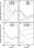 |
Fig. 3 The same as Fig. 1, but for the average magnetic field in the PWN. Note that the magnetic field strength at the inner boundary of the computational domain has been normalised to unity. |
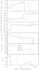 |
Fig. 4 From top to bottom: radial profiles of the magnetic field strength B, density ρ, pressure P, speed v (− v indicates a velocity in the opposite direction), and Mach number at three different times: 1000 yr (solid line), 3000 yr (dotted line), and 5000 yr (dashed line). The profiles shown are for the L0 = 1038 erg s-1, τ = 3000 yr and ρism = 10-24 gcm-3 scenario. Note that B has again been normalised to unity at the inner boundary. |
Figure 3 shows the temporal evolution of the average
magnetic field,  ,
in the PWN, defined as the region
Rts ≤ r ≤ Rpwn.
The solutions correspond to those shown in Figs. 1
and 2. If the magnetic energy in the PWN is not
transferred to the particles, then the conservation of magnetic flux implies that the
evolution of
should be related to the evolution of Rpwn. A comparison of
Figs. 1 and 3
shows that an increase in Rpwn leads to a decrease in
,
with the opposite also being true. Furthermore, the rate of change in
Rpwn is also reflected in the rate of change in
.
,
in the PWN, defined as the region
Rts ≤ r ≤ Rpwn.
The solutions correspond to those shown in Figs. 1
and 2. If the magnetic energy in the PWN is not
transferred to the particles, then the conservation of magnetic flux implies that the
evolution of
should be related to the evolution of Rpwn. A comparison of
Figs. 1 and 3
shows that an increase in Rpwn leads to a decrease in
,
with the opposite also being true. Furthermore, the rate of change in
Rpwn is also reflected in the rate of change in
.
Before the interaction with the reverse shock, it is possible to derive a simple
time-dependence for
since the expansion of Rpwn is described by a power-law. From
the conservation of magnetic flux it follows that 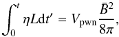 (15)where
η is the fraction of spin-down luminosity converted to magnetic energy
and
(15)where
η is the fraction of spin-down luminosity converted to magnetic energy
and  is the volume
of the PWN. Note that the integral in Eq. (15) represents the total amount of magnetic energy injected into the PWN over
the time interval 0 ≤ t′ ≤ t. According to
Eq. (9), if
t ≲ τ, then L can be approximated as
constant, reducing the integral in Eq. (15) to L0t. Lastly, using
Rpwn ∝ tα it
becomes possible to reduce Eq. (15) to
is the volume
of the PWN. Note that the integral in Eq. (15) represents the total amount of magnetic energy injected into the PWN over
the time interval 0 ≤ t′ ≤ t. According to
Eq. (9), if
t ≲ τ, then L can be approximated as
constant, reducing the integral in Eq. (15) to L0t. Lastly, using
Rpwn ∝ tα it
becomes possible to reduce Eq. (15) to
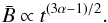 (16)For the values
α = 1.1−1.3, as derived from Fig. 1, the evolution of the average magnetic field in Fig. 3 (before the interaction with the reverse shock) can be described by
(16)For the values
α = 1.1−1.3, as derived from Fig. 1, the evolution of the average magnetic field in Fig. 3 (before the interaction with the reverse shock) can be described by
 ,
where β = 1.15−1.45. The same arguments have also been used by Reynolds & Chevalier (1984) to derive the
evolution of .
For reference, the line
,
where β = 1.15−1.45. The same arguments have also been used by Reynolds & Chevalier (1984) to derive the
evolution of .
For reference, the line  is also shown in Fig. 3. For subsequent times, it is
difficult to characterise the evolution of
with a simple expression as the evolution of Rpwn becomes more
complex.
is also shown in Fig. 3. For subsequent times, it is
difficult to characterise the evolution of
with a simple expression as the evolution of Rpwn becomes more
complex.
3.4. Radial profiles of the fluid quantities
It is also useful to investigate the evolution of the different fluid quantities, especially for times before and after the interaction of Rpwn with the reverse shock. The radial profiles of the fluid quantities at three different times are shown in Fig. 4, corresponding to the scenario L0 = 1038 erg s-1, τ = 3000 yr and ρism = 10-24 gcm-3.
The magnetic profile (top panel) is useful for identifying the various components of the PWN. The radial distance where B falls off to zero indicates the position of Rpwn, while a sharp increase in B indicates the position of Rts (a shock compresses B over a very small region). The B ∝ 1/r decrease before the termination shock is due to the assumption of an azimuthal magnetic field at the inner boundary of the computational domain. An interesting feature of the magnetic field is the increase in strength after Rts, related to the decrease in velocity (see Panel 4). A similar effect occurs in our local heliosphere, with the enhancement known as the Axford-Cranfill effect (Cranfill 1971; Axford 1972). A magnetic wall emerges from the solar wind termination shock, arising from the amplification of the heliospheric magnetic field’s azimuthal component, which in turn is caused by the flow deceleration and the convection to higher latitudes (e.g. Zank 1999).
Using the density profile, Panel 2, allows one to distinguish the different components of the composite remnant. The low density region represents the PWN, and the larger density region the ejecta. The t = 1000 yr profile shows two peaks at r ~ 5 pc and r ~ 7 pc, with these peak respectively representing the reverse and forward shock of the SNR. For larger r values, the constant density region delineates the ISM. Comparing the density profiles of the various times with the position of Rpwn, as defined by Panel 1, shows that there is a region just behind Rpwn where the density increases significantly. This can be heuristically viewed as being a result of Rpwn interacting with the denser ejecta, leading to a pile-up of PWN material. Such an explicit distinction is, however, difficult to make in a one-fluid model.
Panel 3 shows that the pressure behind the reverse shock is lower than both the pressure in the PWN and the SNR shock. It is the pressure difference between the ejecta and shock that eventually leads to the reverse shock propagating back towards the pulsar. After the interaction with the reverse shock, the difference in pressure between the PWN and the ejecta decreases, reducing the PWN expansion rate (see Fig. 1).
Apart from compressing the PWN (and consequently enhancing B), the interaction between the reverse shock and Rpwn drives a reflection wave through the PWN, as illustrated in Panel 5. Lastly, Panel 6 shows that the outer edge of the PWN initially expands supersonically into the ejecta, becoming sub-sonic once the reverse shock has passed.
4. Motivation for the kinematic appraoch
A more correct treatment of the present problem should take into account the effect that the magnetic pressure has on the evolution of the PWN. An ideal approach would be to use an axisymmetric, 2.5-dimensional MHD model, similar to the one presented by Van der Swaluw (2003). However, since these models tend to be computationally expensive, it becomes difficult to do an extensive parameter as presented in Figs. 1–3. The aim of this section is to motivate that a hydrodynamic model with a kinematic approach is a useful approximation when the ratio of magnetic to particle energy is below σ < 0.01. To obtain an estimate of the accuracy, the one-dimensional model presented in the previous section is used, with the difference that the magnetic pressure is calculated at every time step, and added to the total pressure. Similar to the kinematic scenario, this approach has the limitation that it does not produce the required deviations from spherical symmetry. Even though the same model is used, including the effect of the magnetic pressure significantly increases the computational time. The simulations are therefore limited to the single scenario L0 = 1040 erg s-1, τ = 300 yr, Mej = 8 M⊙ and ρism = 10-24 gcm-3, with the PWN evolution only calculated up to t = 1000 yr.
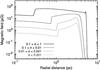 |
Fig. 5 Radial profile of the PWN magnetic field after t = 1000 yr for various values of σ. A range is specified as the values are not constant in the PWN. The plots are for the L0 = 1040 erg s-1, τ = 300 yr, Mej = 8 M⊙ and ρism = 10-24 gcm-3 scenario. |
Figure 5 shows the radial profile of the magnetic field for various values of σ. Note that this value is not constant throughout the nebula, but varies with position. The ranges given in the legend of the figure correspond to the possible values that σ can assume for a given scenario, with σ < 0.001 representing the hydrodynamic/kinematic limit. Comparing the hydrodynamic limit with the 0.001 ≤ σ ≤ 0.01 scenario shows that increase in the magnetic pressure does not lead to a significant change in the size of the PWN. Apart from a larger magnetic field, these two scenarios also predict a very similar magnetic field profile. A significant deviation from the hydrodynamic results only appears when σ ≥ 0.01.
When the magnetic pressure is relatively unimportant (i.e. a low σ value), the compression ratio of the termination shock is large, and the magnetic field is enhanced across the shock. Additionally, the flow speed decreases towards the boundary of the PWN, leading to an continual increase in B as a function of position. By contrast, a larger σ value decreases the compression ratio, resulting in a post-shock magnetic field that decreases as a function of position, with the rate of decrease slightly smaller than the pre-shock value of B ∝ 1/r. This decrease is caused by an acceleration of the post-shock fluid, in turn caused by the gradient of the magnetic pressure.
An increasing in magnetic pressure is sufficient to change the speed of the longitudinal pressure waves, leading to a change in the PWN evolution. A stronger magnetic field at the inner boundary increase the size of the PWN, but also exerts a stronger pressure on Rts, pushing it closer to the pulsar. Note that the effect of magnetic pressure on the PWN evolution may vary when different assumptions are made regarding the initial conditions of the SNR and the boundary conditions of the PWN.
For large σ values, the decreasing magnetic profile in Fig. 5 qualitatively agrees with the steady-state MHD solutions presented by Kennel & Coroniti (1984). On the other hand, these authors found that the post-shock magnetic field increases to a maximum at a few termination shock radii, followed by a decrease towards the outer boundary of the PWN when σ ~ 0.001. Panel 1 in Fig. 4 shows that the kinematic approach predicts a similar character for magnetic field character in the inner part of the PWN, provided that the reverse shock has reached Rpwn. The main difference, compared to the steady-state results of Kennel & Coroniti (1984), is that the magnetic field in Fig. 4 increases again in the outer parts of the PWN. Spherically-symmetric MHD simulations, extending up to t = 1500 yr, have also been performed by Bucciantini et al. (2004b) for the case σ < 0.003. The results of these authors predict a magnetic field that increases with position, qualitatively similar to the results in Fig. 5.
For completeness, the corresponding radial profiles of the flow velocity are shown in Fig. 6. To improve visibility, the velocity of the various profiles have been artificially reduced, with the exception of the 0.001 ≤ σ ≤ 0.01 scenario. The unaltered solutions all have a velocity of c at the inner boundary. From Fig. 6 it can be seen that the hydrodynamic limit and the 0.001 ≤ σ ≤ 0.01 have similar flow velocities and radial profiles. Furthermore, when 0.1 ≤ σ ≤ 1, the flow velocity is almost constant throughout the nebula, in agreement with the predictions made by Kennel & Coroniti (1984).
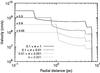 |
Fig. 6 Radial profiles of the flow velocity corresponding to the scenarios in Fig. 5. To enhance clarity, the velocities for the various σ values have been multiplied by different factors. All velocities originally have a value of c at the inner boundary of the computational domain. |
5. Evolution in a non-uniform interstellar medium
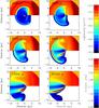 |
Fig. 7 SNR-PWN system evolving in an interstellar medium with a density of ρism = 10-24 gcm-3, with a higher density region, ρism = 10-23 gcm-3 located at x = 5 pc. The results correspond to the Mej = 3 M⊙, τ = 3000 yr, and L0 = 1039 erg s-1 scenario. The top halves of the panels show the density, and the bottom halves the magnetic field. The different panels represent snapshots of the evolution at various times. The time shown in the top-left corner of the panels correspond to the time elapsed after the initial explosion. |
The ISM is very often inhomogeneous, and it is of particular interest to study the evolution of a composite remnant expanding into regions of varying density (e.g. due to the presence of a molecular cloud). The aim is not to investigate any particular object or region, but rather to show some interesting end-result scenarios which can occur. The initial and boundary conditions for this scenario are identical to those described in Sect. 2, with the difference that the ISM has a discontinuous increase in density at a specified distance from the origin of the supernova explosion.
It is well-known that an interaction between a shock front and a discontinuity (CD) separating fluids of different densities leads to a refraction of the shock (e.g. Colella et al. 1989). In the simplest case the original shock front will be refracted into a wave that travels into the transmission medium, and a wave that is reflected back into the incident medium (e.g. Colella et al. 1989). Depending on a number of factors, the transmitted and reflected waves can either be in the form of a shock, an expansion, or a number of complicated wave structures (e.g. Nourgaliev et al. 2005; Delmont 2010). One would therefore expect that the interaction of the forward shock of the SNR with the molecular cloud should lead to a similar wave pattern.
Although difficult to predict the exact character of the refraction, Delmont (2010) found that the most important parameters controlling the refraction are the angle of incidence between the shock front and CD, the Mach number of the initial shock in the incident medium, and the ratio of the densities on opposite sides of the CD. Additionally, if a magnetic field is present, the value of the plasma β, can also influence the interaction (Delmont 2010).
An important feature of the interaction of an oblique shock with a CD is the formation of Richtmeyr-Meshkov vorticity instabilities at the CD (e.g. Colella et al. 1989; Nourgaliev et al. 2005; Delmont 2010). As previously discussed, the set-up used for the present numerical model is such that it does not allow for the development of Rayleigh-Taylor instabilities. The same is also true for the development of fine-scale refraction patterns and Richtmeyr-Meshkov instabilities. It is emphasised that the aim of the present numerical simulations is to obtain an understanding of the evolution of the large-scale structure of the PWN-SNR system in a non-uniform environment.
For the scenario presented in Fig. 7, the SNR evolves into an ISM with a density of ρism = 10-24 gcm-3. At x = 5 pc from the position of the initial explosion, the density of the ISM is larger by a factor 10, i.e. ρism = 10-23 gcm-3. The mass of the ejecta is Mej = 3 M⊙, the spin-down time-scale τ = 3000 yr, and the initial luminosity of the pulsar L0 = 1039 erg s-1.
After roughly t = 2000 yr has elapsed, the forward shock reaches the denser region at x = 5 pc. The sound speed in the incident ISM (x < 5 pc) is larger than the sound speed in the transmission ISM (x ≥ 5 pc), and the interaction is thus classified as fast-slow (e.g. Colella et al. 1989). A study of the radial profiles (not shown) shows that the interaction leads to a sub-sonic wave that is reflected back into the incident ISM, and a sub-sonic wave that is transmitted into the denser ISM. When the reflection wave interacts with the PWN, the t = 3000 yr panel shows that the part of the PWN located at x > 0 pc is compressed and pushed back towards the pulsar (located at the origin). As time evolves, the reverse shock flows over an increasingly larger part of the PWN, deforming initially spherical nebula into a bullet-shaped PWN.
The initial compression, as well as the subsequent deformation, leads to a pile-up of the magnetic field in the nose of the PWN, as well as long the edge of the nebula. After t = 4000 yr, an additional enhancement of the magnetic field also becomes visible at the opposite edge of the PWN. The PWN material transported away from the pulsar (in the − x direction) by the reflection wave is decelerated by the supernova ejecta, leading to an additional pile-up of the magnetic field. For times t > 6000 yr, the decrease in the pulsar’s spin-down luminosity becomes important, leading to a pressure gradient between the PWN and ejecta/ISM. A wind is created that continually flows over the PWN (t = 12 000 yr and t = 20 000 yr panels), resulting in a further compression of the magnetic field along the edge of the nebula.
For the second scenario presented in Fig. 8, the ISM has a density ρism = 10-24 g cm-3, with a factor thousand increase at x = 5 pc, i.e. ρism = 10-21 g cm-3. The mass of the ejecta and spin-down time-scale is again chosen as Mej = 3 M⊙ and τ = 3000 yr, respectively, while the initial luminosity is reduced by a factor ten to L0 = 1038 erg s-1. Note that the scale of the magnetic field in Fig. 8 is different to that of Fig. 7.
The interaction of the sub-sonic reflection wave with the PWN is significantly more pronounced, with the PWN being almost crushed by the wave. A closer look at the t = 12 000 yr panel reveals that some of the PWN material initially transported in the − x-direction (as a result of the reflection wave) is now flowing in the opposite direction. The primary reflection wave flows through the lower density PWN, eventually reaching the discontinuity between the PWN and higher density supernova ejecta. This results in the formation of a secondary reflection wave that propagates in the opposite direction. This effect is not visible in Fig. 7 since a larger L0 implies a larger pressure in the PWN, which would cancel out such an effect. As the secondary wave propagates towards the pulsar, the magnetic field is dragged along with it, leading to a pile-up of the magnetic field. The t = 20 000 yr panel shows that this magnetic cloud is eventually pushed in the − x-direction. The largest magnetic field is therefore found in a region that is spatially uncorrelated with the position of the pulsar.
6. Summary and conclusions
This paper investigates the evolution of a composite supernova remnant for a number of scenarios, with an emphasis on the evolution of the PWN. A hydrodynamic model is used for the simulations, with the magnetic field included in a kinematic fashion. In this approach the interaction between the fluid and magnetic field is strictly one-sided as the effect of the magnetic field on the flow is neglected. The kinematic results were compared to a more correct treatment of the problem where the effect of the magnetic pressure is included. It was found that the two approaches give similar results when the ratio of magnetic to particle energy is σ < 0.01.
One of the aims of the paper is to determine the effect that the initial luminosity (L0) and the spin-down time-scale (τ) of the pulsar, together with the mass of the stellar ejecta (Mej) and density of the ISM (ρism) have on the evolution of a spherically-symmetric composite remnant expanding into a homogeneous ISM. It was found that the evolution of the PWN is primarily determined by L0 and ρism, while the influence of Mej is almost negligible. It was also found that τ only has an influence on the evolution when the spin-down time-scale is smaller than the time needed for the reverse shock to reach the outer boundary of the nebula, Rpwn.
For the L0 = 1040 erg s-1, τ = 3000 yr scenario, the interaction between the PWN and reverse shock only leads to a decrease in the expansion rate of Rpwn. For smaller L0 values, the PWN undergoes a compression phase, with a decrease in L0 leading to a larger compression. Furthermore, a larger ISM density decreases the time needed by the reverse shock to reach Rpwn, thereby markedly reducing the size of the PWN.
The parameter study further found that the termination shock radius, Rts, increases with time until the PWN encounters the reverse shock. The latter sends a reflection wave through the PWN towards the pulsar, resulting in a decrease of Rts. The evolution of Rts is an important quantity as it may help to determine the progress of the reverse shock through the PWN. Additionally, the ratio of the PWN boundary to the termination shock radius, Rts/Rpwn, has also previously been used to derive the initial spin-period, P0, for a number of pulsars (Van der Swaluw 2003).
Studies of the evolution of the average magnetic field are important when attempting to understand so-called “dark sources”, i.e. TeV γ-ray sources without a synchrotron counterpart (Aharonian et al. 2008). From Fig. 3 it can be seen that a rapid expansion of the PWN (L0 = 1040 erg s-1, τ = 3000 yr) leads to a significant decrease in the average magnetic field as a function of time, which in turn will lead to a faint synchrotron source.
The evolution of Rpwn and the average magnetic field are of particular importance to the one-zone (spatially-independent) radiation models that are often used to derive PWN parameters (e.g. Zhang et al. 2008; Fang & Zhang 2010; Tanaka & Takahara 2011). Additionally, the radial profiles of the magnetic field and flow velocity can also be incorporated into spatially-dependent transport models that describe the evolution of the non-thermal particle spectrum in the nebula (Vorster & Moraal 2013).
The simulations of a composite remnant evolving into an inhomogeneous ISM show that an initially spherical PWN will evolve into a bullet-shaped nebula. This is in agreement with observations since most PWN are observed as offset from the pulsar (for a summary of observations, see e.g. Gaensler & Slane 2006; De Jager & Djannati-Ataï 2009). The simulations further show that the interaction between the nebula and the asymmetric reverse shock (resulting from an inhomogeneous ISM) leads to an enhancement of the the magnetic field at the edge of the PWN. Recent Suzaku observations of the Vela PWN reveal an X-ray nebula that extends beyond the 3° × 2° radio nebula (Katsuda et al. 2011). This is somewhat surprising as synchrotron radiation is expected to effectively cool the X-ray producing leptons, leading to an X-ray nebula that is smaller than the radio counterpart. Although Katsuda et al. (2011) favour a scenario in which these leptons effectively diffuse outward, the authors do not rule out a scenario in which lower energy leptons produce X-rays as a result of an increase in the magnetic field at the edge of the nebula.
Decreasing the value of L0, while simultaneously increasing the density gradient in the ISM, leads to the creation of a magnetic “cloud” in a region that is spatially separated from the pulsar. The associated synchrotron emission will be enhanced, leading to a brighter region that is unconnected with the present position of the pulsar.
Acknowledgments
The authors are grateful for partial financial support granted to them by the South African National Research Foundation (NRF) and by the Meraka Institute as part of the funding for the South African Centre for High Performance Computing (CHPC).
References
- Aharonian, F., Akhperjanian, A. G., Bazer-Bachi, A. R., et al. 2006, A&A, 449, 223 [NASA ADS] [CrossRef] [EDP Sciences] [Google Scholar]
- Aharonian, F., Akhperjanian, A. G., Barres de Almeida, U., et al. 2008, A&A, 477, 353 [Google Scholar]
- Arzoumanian, Z., Chernoff, D. F., & Cordes, J. M. 2002, ApJ, 568, 289 [NASA ADS] [CrossRef] [Google Scholar]
- Axford, W. I. 1972, in Solar Wind, eds. C. P. Sonett, P. J. Coleman, & J. M. Wilcox, 598 [Google Scholar]
- Blondin, J. M., & Ellison, D. C. 2001, ApJ, 560, 244 [NASA ADS] [CrossRef] [Google Scholar]
- Blondin, J. M., Wright, E. B., Borkowski, K. J., & Reynolds, S. P. 1998, ApJ, 500, 342 [NASA ADS] [CrossRef] [Google Scholar]
- Blondin, J. M., Chevalier, R. A., & Frierson, D. M. 2001, ApJ, 563, 806 [NASA ADS] [CrossRef] [Google Scholar]
- Borkowski, K. J., Blondin, J. M., & McCray, R. 1997, ApJ, 477, 281 [NASA ADS] [CrossRef] [Google Scholar]
- Bucciantini, N. 2002, A&A, 387, 1066 [NASA ADS] [CrossRef] [EDP Sciences] [Google Scholar]
- Bucciantini, N., Blondin, J. M., Del Zanna, L., & Amato, E. 2003, A&A, 405, 617 [NASA ADS] [CrossRef] [EDP Sciences] [Google Scholar]
- Bucciantini, N., Amato, E., Bandiera, R., Blondin, J. M., & Del Zanna, L. 2004a, A&A, 423, 253 [NASA ADS] [CrossRef] [EDP Sciences] [Google Scholar]
- Bucciantini, N., Bandiera, R., Blondin, J. M., Amato, E., & Del Zanna, L. 2004b, A&A, 422, 609 [NASA ADS] [CrossRef] [EDP Sciences] [Google Scholar]
- Bucciantini, N., Amato, E., & Del Zanna, L. 2005, A&A, 434, 189 [NASA ADS] [CrossRef] [EDP Sciences] [Google Scholar]
- Chevalier, R. A. 1977, ARA&A, 15, 175 [NASA ADS] [CrossRef] [Google Scholar]
- Chevalier, R. A. 2005, ApJ, 619, 839 [NASA ADS] [CrossRef] [Google Scholar]
- Colella, P., Henderson, L. F., & Puckett, E. G. 1989, in 9th AIAA Computational Fluid Dynamics Conference, eds. D. B. Bliss, & W. O. Miller, 426 [Google Scholar]
- Cranfill, C. 1971, Ph.D. Thesis, University of California, San Diego [Google Scholar]
- De Jager, O. C., & Djannati-Ataï, A. 2009, ASSL, ed. W. Becker, 357, 451 [Google Scholar]
- Decourchelle, A., Ellison, D. C., & Ballet, J. 2000, ApJ, 543, L57 [NASA ADS] [CrossRef] [Google Scholar]
- Del Zanna, L., Amato, E., & Bucciantini, N. 2004, A&A, 421, 1063 [NASA ADS] [CrossRef] [EDP Sciences] [Google Scholar]
- Delmont, P. 2010, Ph.D. Thesis, Arenberg Doctoral School of Sciene, Engineering and Technology, Katholieke Unversiteit, Leuven [Google Scholar]
- Dwarkadas, V. V., & Chevalier, R. A. 1998, ApJ, 497, 807 [NASA ADS] [CrossRef] [Google Scholar]
- Ellison, D. C., Decourchelle, A., & Ballet, J. 2004, A&A, 413, 189 [NASA ADS] [CrossRef] [EDP Sciences] [Google Scholar]
- Fang, J., & Zhang, L. 2010, A&A, 515, A20 [NASA ADS] [CrossRef] [EDP Sciences] [Google Scholar]
- Faucher-Giguère, C.-A., & Kaspi, V. M. 2006, ApJ, 643, 332 [NASA ADS] [CrossRef] [Google Scholar]
- Ferreira, S. E. S., & De Jager, O. C. 2008, A&A, 478, 17 [NASA ADS] [CrossRef] [EDP Sciences] [Google Scholar]
- Ferreira, S. E. S., & Scherer, K. 2006, ApJ, 642, 1256 [NASA ADS] [CrossRef] [Google Scholar]
- Gaensler, B. M., & Slane, P. O. 2006, ARA&A, 44, 17 [NASA ADS] [CrossRef] [Google Scholar]
- Horns, D., Aharonian, F., Santangelo, A., Hoffmann, A. I. D., & Masterson, C. 2006, A&A, 451, L51 [NASA ADS] [CrossRef] [EDP Sciences] [Google Scholar]
- Jun, B.-I., & Jones, T. W. 1999, ApJ, 511, 774 [NASA ADS] [CrossRef] [Google Scholar]
- Kargaltsev, O., & Pavlov, G. G. 2008, in 40 Years of Pulsars: Millisecond Pulsars, Magnetars and More, eds. C. Bassa, Z. Wang, A. Cumming, & V. M. Kaspi, AIP Conf. Ser., 983, 171 [Google Scholar]
- Katsuda, S., Mori, K., Petre, R., et al. 2011, PASJ, 63, 827 [Google Scholar]
- Kennel, C. F., & Coroniti, F. V. 1984, ApJ, 283, 694 [NASA ADS] [CrossRef] [Google Scholar]
- LeVeque, R. J. 2002, Finite Volume Methods for Hyperbolic Problems (Cambridge University Press) [Google Scholar]
- McKee, C. F. 1974, ApJ, 188, 335 [NASA ADS] [CrossRef] [Google Scholar]
- McKee, C. F., & Truelove, J. K. 1995, Phys. Rep., 256, 157 [NASA ADS] [CrossRef] [Google Scholar]
- Nourgaliev, R. R., Sushchikh, S. Y., Dinh, T. N., & Theofanous, T. G. 2005, Intern. J. Multiphase Flow, 31, 969 [CrossRef] [Google Scholar]
- Rees, M. J., & Gunn, J. E. 1974, MNRAS, 167, 1 [NASA ADS] [CrossRef] [Google Scholar]
- Reynolds, S. P., & Chevalier, R. A. 1984, ApJ, 278, 630 [NASA ADS] [CrossRef] [Google Scholar]
- Scherer, K., & Ferreira, S. E. S. 2005, Astrophys. Space Sci. Trans., 1, 17 [NASA ADS] [CrossRef] [Google Scholar]
- Sedov, L. I. 1959, Similarity and Dimensional Methods in Mechanics (Academic Press) [Google Scholar]
- Shigeyama, T., & Nomoto, K. 1990, ApJ, 360, 242 [NASA ADS] [CrossRef] [Google Scholar]
- Tanaka, S. J., & Takahara, F. 2011, ApJ, 741, 40 [NASA ADS] [CrossRef] [Google Scholar]
- Tang, S., & Wang, Q. D. 2005, ApJ, 628, 205 [NASA ADS] [CrossRef] [Google Scholar]
- Tenorio-Tagle, G., Rozyczka, M., Franco, J., & Bodenheimer, P. 1991, MNRAS, 251, 318 [NASA ADS] [CrossRef] [Google Scholar]
- Thornton, K., Gaudlitz, M., Janka, H.-T., & Steinmetz, M. 1998, ApJ, 500, 95 [NASA ADS] [CrossRef] [Google Scholar]
- Trac, H., & Pen, U.-L. 2003, PASP, 115, 303 [NASA ADS] [CrossRef] [Google Scholar]
- Truelove, J. K., & McKee, C. F. 1999, ApJ, 120, 299 [Google Scholar]
- Van der Swaluw, E. 2003, A&A, 404, 939 [NASA ADS] [CrossRef] [EDP Sciences] [Google Scholar]
- Van der Swaluw, E., & Wu, Y. 2001, ApJ, 555, L49 [NASA ADS] [CrossRef] [Google Scholar]
- Van der Swaluw, E., Achterberg, A., Gallant, Y. A., & Tóth, G. 2001, A&A, 380, 309 [NASA ADS] [CrossRef] [EDP Sciences] [Google Scholar]
- Van der Swaluw, E., Achterberg, A., Gallant, Y. A., Downes, T. P., & Keppens, R. 2003, A&A, 397, 913 [NASA ADS] [CrossRef] [EDP Sciences] [Google Scholar]
- Van der Swaluw, E., Downes, T. P., & Keegan, R. 2004, A&A, 420, 937 [NASA ADS] [CrossRef] [EDP Sciences] [Google Scholar]
- Vorster, M. J., & Moraal, H. 2013, accepted [Google Scholar]
- Woltjer, L. 1972, ARA&A, 10, 129 [NASA ADS] [CrossRef] [Google Scholar]
- Woosley, S., & Janka, T. 2005, Nat. Phys., 1, 147 [Google Scholar]
- Zank, G. P. 1999, Space Sci. Rev., 89, 413 [NASA ADS] [CrossRef] [Google Scholar]
- Zhang, L., Chen, S. B., & Fang, J. 2008, ApJ, 676, 1210 [NASA ADS] [CrossRef] [Google Scholar]
All Figures
|
Fig. 1 Model solutions for the evolution of the outer boundary of a spherically-symmetric PWN in a homogeneous ISM. A basis parameter set is chosen as L0 = 1039 erg s-1, τ = 3000 yr, Mej = 12 M⊙, and ρism = 10-25 gcm-3, with the solution represented by a short-dashed line in panels a)–d). The other solutions were obtained by using the basis parameters, while varying the parameters listed in the legends of the figures. The ◇ symbol represents the time when the reverse shock reaches Rpwn. Also shown in panels a) and b) is the evolution of the forward shock of the SNR. |
| In the text | |
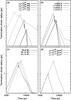 |
Fig. 2 The same as Fig. 1, but for the termination shock radius, Rts. |
| In the text | |
|
Fig. 3 The same as Fig. 1, but for the average magnetic field in the PWN. Note that the magnetic field strength at the inner boundary of the computational domain has been normalised to unity. |
| In the text | |
|
Fig. 4 From top to bottom: radial profiles of the magnetic field strength B, density ρ, pressure P, speed v (− v indicates a velocity in the opposite direction), and Mach number at three different times: 1000 yr (solid line), 3000 yr (dotted line), and 5000 yr (dashed line). The profiles shown are for the L0 = 1038 erg s-1, τ = 3000 yr and ρism = 10-24 gcm-3 scenario. Note that B has again been normalised to unity at the inner boundary. |
| In the text | |
|
Fig. 5 Radial profile of the PWN magnetic field after t = 1000 yr for various values of σ. A range is specified as the values are not constant in the PWN. The plots are for the L0 = 1040 erg s-1, τ = 300 yr, Mej = 8 M⊙ and ρism = 10-24 gcm-3 scenario. |
| In the text | |
|
Fig. 6 Radial profiles of the flow velocity corresponding to the scenarios in Fig. 5. To enhance clarity, the velocities for the various σ values have been multiplied by different factors. All velocities originally have a value of c at the inner boundary of the computational domain. |
| In the text | |
|
Fig. 7 SNR-PWN system evolving in an interstellar medium with a density of ρism = 10-24 gcm-3, with a higher density region, ρism = 10-23 gcm-3 located at x = 5 pc. The results correspond to the Mej = 3 M⊙, τ = 3000 yr, and L0 = 1039 erg s-1 scenario. The top halves of the panels show the density, and the bottom halves the magnetic field. The different panels represent snapshots of the evolution at various times. The time shown in the top-left corner of the panels correspond to the time elapsed after the initial explosion. |
| In the text | |
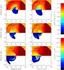 |
Fig. 8 The same as Fig. 7, except L0 = 1038 erg s-1 and ρism = 10-21 gcm-3 for the “cloud”. |
| In the text | |
Current usage metrics show cumulative count of Article Views (full-text article views including HTML views, PDF and ePub downloads, according to the available data) and Abstracts Views on Vision4Press platform.
Data correspond to usage on the plateform after 2015. The current usage metrics is available 48-96 hours after online publication and is updated daily on week days.
Initial download of the metrics may take a while.