| Issue |
A&A
Volume 550, February 2013
|
|
|---|---|---|
| Article Number | L9 | |
| Number of page(s) | 4 | |
| Section | Letters | |
| DOI | https://doi.org/10.1051/0004-6361/201220766 | |
| Published online | 29 January 2013 | |
Reversals of the solar dipole
1 School of Mathematics, University of Manchester, Oxford Road, Manchester, M13 9PL, UK
e-mail: This email address is being protected from spambots. You need JavaScript enabled to view it.
2 Institute for Solar-Terrestrial Physics, PO Box 291, 664033 Irkutsk, Russia
3 Pulkovo Astronomical Observatory, 196140 St. Petersburg, Russia
4 Department of Physics, Moscow University, 119992 Moscow, Russia
Received: 20 November 2012
Accepted: 31 December 2012
Abstract
Context. During a solar magnetic field reversal the magnetic dipole moment does not vanish, but migrates between poles, in contradiction to the predictions of mean-field dynamo theory.
Aims. We try to explain this as a consequence of magnetic fluctuations.
Methods. We used the statistics of fluctuations to estimate observable signatures.
Results. Simple statistical estimates, taken with results from mean-field dynamo theory, suggest that a non-zero dipole moment may persist through a global field reversal.
Conclusions. Fluctuations in the solar magnetic field may play a key role in explaining reversals of the solar dipole.
Key words: Sun: dynamo / Sun: activity / Sun: surface magnetism / dynamo
© ESO, 2013
1. Introduction
Magnetic activity is a quasi-regular cyclic process during the course of which the solar magnetic field changes its polarity in each nominal 11-year cycle. This cyclic activity is usually explained as a manifestation of solar dynamo action somewhere within the solar interior. The Sun and its activity are more or less axially symmetric. Of course, the distribution of sunspots is not completely symmetric because of, e.g., the discrete nature of this tracer of solar activity. However, if distributions of this and other tracers of solar activity are averaged over a reasonable time interval, they becomes almost axisymmetric, and at any time surface deviations from axisymmetry in the form of preferred longitudes are about 10% (e.g. Berdyugina et al. 2006). This is why a description of the solar activity in terms of axisymmetric dynamo models seems to be a reasonable step, and nonaxisymmetric features can be considered as small perturbations. Of course, a deeper understanding of solar activity in terms of direct numerical simulations for detailed solar magnetic configurations which automatically include small-scale nonaxisymmtric features, is a very desirable subsequent step (see, e.g. Brown et al. 2010, whose model has a dipole moment whose evolution does hint at some of the desired features).
The scheme described above looks plausible. However, it implies that the mean magnetic dipole moment of the magnetic field vanishes during the course of each reversal: axisymmetric spherical mean-field dynamos have two possible directions of their dipole magnetic moment, parallel or anti-parallel to the rotation axis. Mean-field solar dynamo models exploit this idea massively. Almost all mean-field models assume that the magnetic dipole moment vanishes at the instant of field reversal.
On the other hand observers insist that in reality the magnitude of the solar magnetic dipole moment is reduced at the times of its reversal, but does not vanish exactly. Instead its direction moves continuously from one pole to the other on a quite complicated trajectory, which varies from one reversal to the other (e.g. Antonucci 1974; Zhukov & Veselovsky 2000; Livshits & Obridko 2006). The topic was later investigated in detail by DeRosa et al. (2012) who provided further convincing evidence concerning the migration of the solar magnetic dipole moment from one pole to the other during the course of a reversal.
The solar dynamo is not fully axisymmetric, and weak deviations from axial symmetry in solar hydrodynamics and/or dynamo generation can be used to explain the relatively weak dipole magnetic moment at the times of reversals. The point is, however, that the mean-field solar dynamo is known to be very robust and it is extremely difficult to excite a quite substantial nonaxisymmetric magnetic field in a solar type mean-field dynamo.
A radically different viewpoint is that that there is no need to describe solar magnetic field evolution in the framework of mean-field dynamos and that if such models have problems, it is time to move to direct numerical simulations of the non-averaged induction equation, e.g. along the lines of Brown et al. (2010). We feel, however, that it would be much better to attempt to resolve the problem rather to ignore it. Mean-field dynamo theory is too useful a tool in understanding these phenomena to be lightly discarded.
We note that the reversals with nonvanishing magnetic moment touches on one more related problem. The point is that an inclined magnetic moment creates a quadrupole magnetic field mode in addition to the nonaxisymmetric one. The appearance of a quadrupole component was convincingly addressed in the context of interest by DeRosa et al. (2012). We note, however, that dynamo excitation of a quadrupole dynamo configuration by a spherical dynamo is much less problematic (see e.g. Moss et al. 2008a,b) than excitation of nonaxisymmetric configurations.
The aim of this paper is to give an interpretation of observations discussed in DeRosa et al. (2012) in the context of nonaxisymmetric dynamo configurations and spherical mean-field dynamos. We start by revisiting the problem of the existence of nonaxisymmetric solutions in the framework of mean-field dynamos, and confirm that it struggles to explain the phenomenology under discussion. Then we suggest a minimal extension of mean-field theory, which can explain the phenomenon, by adding explicitly a random (fluctuating) magnetic field component (which is anyway implicitly present in any mean-field dynamo) to the dynamo generated mean field. The irregular nature of the dipole’s motion is strongly suggestive of the input of a random process. We demonstrate that such a model can explain the nonaxisymmetric magnetic dipole migration during the reversals, within the admissible parameter range. DeRosa et al. (2012) provide an accessible background for the ideas developed in this paper. This explanation looks quite straightforward; however, we failed to find previous explicit reference to it in the literature.
2. Searching for nonaxisymmetries
The topic of symmetries of spherical dynamo was extensively addressed in the early years of dynamo studies and the basic message from that epoch still remains valid. In particular, Rädler (1986) and Moss et al. (1991a) investigated spherical dynamo models that permit nonaxisymmetric solutions, and found that solar-type dynamos preferentially excite axisymmetric rather than nonaxisymmetric magnetic fields, and that the axisymmetric solutions are very stable with respect to nonaxisymmetric perturbations. We did rerun some similar models and confirmed the result. A point to be mentioned in the present context is that the lifetime of a nonaxisymmetric perturbation introduced in a dynamo generated axisymmetric magnetic configuration can exceed the reversal time, i.e. if the desired perturbation arises it can survive through the period of reversal.
A dynamo can in some situations excite nonaxisymmetric configurations and efforts were undertaken to include such possibilities in the framework of solar dynamos (e.g. Ruzmaikin et al. 1988; Moss 1999). These isolated attempts are rather exploratory and at the moment they do not provide strong motivation for further reconsideration of significant nonaxisymmetric field generation by more-or-less conventional mean-field solar dynamos. We can note that, for example in Moss (1999) the axisymmetric and nonaxisymmetric field components oscillate in phase.
Note that the issue of possible excitation of a quadrupole axisymmetric magnetic configuration is quite different from that of the existence of nonaxisymmetric solutions. Of course, the solar dynamo is observed normally to excite a dipolar configuration. However, a modest variation in the profiles of the dynamo drivers and/or control parameters can result in excitation of a configuration with quadrupolar symmetry; this problem was recently revisited by Moss et al. (2008a,b), among many others. Moreover, archival solar activity data for the XVIIIth century (Arlt 2009) give a hint that the solar magnetic field then had quadrupolar symmetry (Illarionov et al. 2011). A substantial deviation from dipole symmetry with a significant admixture of a quadrupole field is known to have been present at the end of the Maunder Minimum (Sokoloff & Nesme-Ribes 1994). Nevertheless, the above remarks do not provide evidence for quadrupole-like type features playing a role in solar magnetic field reversals.
We do not give here a detailed verification of the above results, but describe a simple minded numerical experiment. We took as a basis the nonlinear nonaxisymmetric dynamo code described in Berdyugina et al. (2006), with solar rotation law in the “convection zone” proper (fractional radius r ≥ 0.7), isotropic alpha-effect and a rather thick overshoot layer with slightly reduced diffusivity, which allows the angular velocity to become uniform at its base (r = 0.64) in a smooth manner.
First the code was run with slightly supercritical parameters, to obtain a stable, oscillating solution with pure dipole-like parity. In our dimensionless units, the period of oscillation in energy is PE ≈ 0.024 (this would correspond to the “11 yr” sunspot cycle on the Sun). Then a massive alpha-perturbation was imposed in one longitudinal hemisphere, rotating with the angular velocity at the base of the convection zone (r = 0.7), for a time interval of length 0.005 (i.e. about 0.2PE). The perturbation was then switched off. The time evolution of the energies in the axisymmetric and nonaxisymmetric (overwhelmingly in mode m = 1) parts of the field are shown in Fig. 1.
Figure 1 illustrates two relevant points. A nonaxisymmetric perturbation in alpha rapidly generates a (weak) nonaxisymmetric field. When the driver is removed (at time 0.605 in Fig. 1), the nonaxisymmetric field decays with a decay time of about 25% of the cycle period (i.e. of PE). (Because of the disparate magnitudes of the quantities plotted in Fig. 1 the oscillation in the axisymmetric field is barely visible.) We do not pretend that this model is in any way realistic, but it does illustrate the points that a nonaxisymmetic field is quickly established by the perturbation, and decays much more slowly. This is quite consistent with previous studies, which indicate that axisymmetric solutions for αΩ dynamos in spherical geometry are very stable to nonaxisymmetric perturbations, e.g. Rädler (1986); Moss et al. (1991b); see also recent estimates for the decay rate of magnetic structures in Blackman & Subramanian (2013).
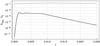 |
Fig. 1 Evolution of energy in the axisymmetric field (upper curve) and nonaxisymmetric field (lower curve). At dimensionless time 0.6, the steadily oscillating axisymmetric solution (period PE ≈ 0.024) is perturbed by the addition of a nonaxisymmetric part in alpha between times 0.6 and 0.605. The nonaxisymmetric perturbation is then removed, and the nonaxisymmetric field decays. |
3. Our scenario: mean field plus fluctuations
A minimal extension of standard mean-field dynamo theory that includes solar magnetic reversals with a nonvanishing magnetic moment can be presented as follows. Mean-field dynamo theory assumes that, apart from the mean magnetic field B, which is considered to be the large-scale magnetic field, magnetic field fluctuations b are also present, so the total magnetic field H = B + b. The mathematical expectation of b is zero but the spatial average of b remains finite. This is because the number of convective cells N, while large, is not so big that the spatial averaging of b (which scales as  ) effectively vanishes.
The number of convective cells N participating in dynamo action in the convection zone can be estimated as follows. Taking for estimates the supergranulation scale as 30 Mm, we find that there are about 104 supergranules at the solar surface or about (5 ~ 7) × 104 in the whole convection zone. However, supergranulation is a surface phenomenon whose spatial scale is probably controlled by the depth of the He++ ionization region (November et al. 1981). The characteristic scales of the deeper convection are larger, so that N ≈ 104 seems to be a reasonable estimate for the number of convection cells in the Sun.
Knowing the magnetic field H we can estimate the dipole magnetic moment m as 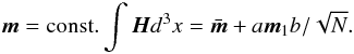 (1)where
  is the magnetic moment of the mean field B, m1 is a random vector of unit length, b is the rms value of the magnetic fluctuations and a is a numerical constant.
Two mechanisms producing fluctuating magnetic fields are known: the small-scale dynamo and the wiggling of large-scale field lines by turbulent convection. The observation-based upper limit on the amplitude of the surface fields produced by the small-scale dynamo in the Sun is only about 3 G (Stenflo 2012a). The contribution of such small fields to the global magnetic dipole moment of Eq. (1) can be neglected in view of the large number N of convective cells. We therefore consider the distortion of global field lines by convection as the primary source of fluctuating fields.
Assume that b is of order of the field strength of the toroidal magnetic field BT. Such an estimate looks plausible in the framework of the standard ideas of mean-field dynamos and is supported by the analysis of unipolar sunspot group statistics (Khlystova & Sokoloff 2010; Sokoloff & Khlystova 2011). The poloidal (polar) field BP of the Sun, which determines  , is ~ 1 G (cf. e.g. Hathaway 2010). The toroidal field near the base of convection zone is believed to be at least 1000 times stronger. Near the surface, however, the toroidal field is probably weaker and the poloidal field inside the convective zone is probably stronger (Kitchatinov & Olemskoy 2012). Taking for estimates BP = 0.03BT and
  we find that the first term in the r.h.s. of Eq. (1) to be several times larger than the second. In other words, it is the contribution of the mean magnetic field that determines the total solar magnetic moment far from the instant of reversal. Of course, the direction of m does not coincide with that of , i.e. the direction of the rotation axis, precisely but the angle θ between m and the rotation axis is quite small, tanθ = 0.1 ~ 0.2, i.e. θ ≈ 5° − 10°.
The situation near the time of magnetic field reversal is quite different. Then vanishes and the total magnetic moment m is determined by the second term in the r.h.s. of Eq. (1). m becomes weak but does not vanish. With the above estimates, the magnetic moment at the instant of reversal becomes several times weaker than its characteristic value far from the reversal epochs.
When the Sun is still far from the instant of reversal, the first term in the r.h.s. of Eq. (1) is larger than the second. If is directed to, say, the North pole, the direction of m is aligned closely with this pole. For the same reason, m is aligned closely to the opposite pole after the reversal, when is again large. The dipole’s track from one pole to the other in course of a reversal is determined by the direction m1, i.e. by the nonaxisymmetric part b of the total magnetic field H. b is a physical field, and convection cannot destroy it immediately. This follows from the results of Sect. II where we find that the flow destroys a nonaxisymmetric field in a time of about 1 − 2 years, and is why the motion from one pole to the other is quasiregular.
To summarize, m is determined by the sum of the dominant fluctuations (nonaxisymmetric) and the mean field contribution (axisymmetric). The nonaxisymmetric fluctuations individually decay on a timescale tD ≲ tr, and their sum is determined predominantly by the most recent several contributions. As the mean field component weakens, changes sign on passing through zero, and then grows again, the total m moves from being directed outwards in one hemisphere to pointing out from the other, on an irregular path essentially determined by the dominant fluctuation.
The relative contribution of the second, fluctuating term in the r.h.s. of Eq. (1) can also be estimated as a ratio of reversal time to the cycle length. Taking 1 − 2 years for the reversal time tr and 11 years for the cycle length, we find again that the fluctuating part of m is up to an order of magnitude smaller than its mean part.
According to Sect. 2 a nonaxisymmetric feature, and in particular m1, can survive for up to 1 − 2 years, i.e. the time tr required for a reversal. On the other hand, the convection turnover time t ∗ estimated for the vortices of the largest scale is 1 − 2 solar rotation (cf. Stix 1991), i.e. a few months – substantially less than the reversal time. Indeed, observers refer to so-called “fast” global changes on that time scale (see e.g. Hoeksema 2006). Magnetic fluctuations, being determined by cumulative action of the velocity field, have a longer memory time, tr, than that of the convection itself (t ∗ ); however, some rapid changes on the time scale t ∗ have to be expected.
The presence of two memory times, tr and t ∗ , can explain the irregular, chaotic track of the magnetic moment during the reversals. Observations (e.g. Livshits & Obridko 2006) demonstrate this feature of the reversals.
4. Discussion
We have demonstrated that a minimal extension of the standard mean-field solar dynamo theory to allow explicitly for fluctuations is sufficient to describe magnetic field reversals with nonvanishing magnetic moment. With this in mind the main concepts of mean-field dynamos can be retained to explain the phenomenology of the solar cycle with reasonable accuracy; further development looks desirable.
The initial formulation of mean-field dynamos included magnetic fluctuations at least implicitly. Hoyng (1987) stressed their role explicitly and Choudhuri (1992), Moss et al. (1992) and Hoyng (1993) applied this idea to explanations of solar cycle variability. The contemporary level of knowledge of fluctuations in the dynamo governing parameters suggests that they may provide a scenario explaining solar Grand Minima (e.g. Moss et al. 2008a,b; Usoskin et al. 2009) and the Waldmaier relations for the time dependence of the solar cycle (Pipin et al. 2012). The idea seems relevant to explaining magnetic reversals also.
Note, that our explanation does not require solar convection to be isotropic, which Hangasoge et al. (2012) suggest might be inapplicable to the real Sun, neither does it appeal to small-scale dynamo action which Stenflo (2012b) argues may also be inapplicable.
Also note that a similar problem is present in the geodynamo. The geomagnetic dipole is currently inclined to the Earth’s rotation axis at an angle θ = 11° and, according to the paleomagnetic data (e.g. Laj et al. 1991) the geomagnetic field has reversed from time to time in geological history, with nonvanishing magnetic dipole moment. It is reasonable to assume that, magnetic fluctuations underlie this phenomenon also.
In summary, recognition of the importance of fluctuations in the solar dynamo mechanism may provide a crucial step to explaining a range of non-periodic phenomena.
Acknowledgments
This work is supported by RFBR grants 12-02-92691_Ind and 12-02-00170, and by MESRF contract 14.518.11.7047. We thank V. Obridko and V. Pavlov for fruitful discussions, and an anonymous referee for pertinent comments.
References
- Antonucci, E. 1974, SUIPR Rep. 570 [Google Scholar]
- Arlt, R. 2009, Sol. Phys., 255, 143 [NASA ADS] [CrossRef] [Google Scholar]
- Berdyugina, S. V., Moss, D., Sokoloff, D., & Usoskin, I. G. 2006, A&A, 445, 703 [NASA ADS] [CrossRef] [EDP Sciences] [Google Scholar]
- Blackman, E. G., & Subramanian, K. 2013, MNRAS, in press [arXiv:1209.2230] [Google Scholar]
- Brown, B. P., Browning, M. K., Brun, A. S., Miesch, M. S., & Toomre, J. 2010, ApJ, 711, 424 [Google Scholar]
- Choudhuri, A. R. 1992, A&A, 253, 277 [NASA ADS] [Google Scholar]
- DeRosa, M. L., Brun, A. S., & Hoeksema, J. T. 2012, ApJ, 757, 96 [Google Scholar]
- Hanasoge, S., Duvall, T. L., & Sreenivasan, K. R. 2012 [arXiv:1206.3173] [Google Scholar]
- Hathaway, D. H. 2010, Liv. Rev. Sol. Phys., 7, 1 [Google Scholar]
- Hoeksema, T. 2006, Adv. Sp. Res., 38, 831 [NASA ADS] [CrossRef] [Google Scholar]
- Hoyng, P. 1987, A&A, 171, 348 [NASA ADS] [Google Scholar]
- Hoyng, P. 1993, A&A, 272, 321 [NASA ADS] [Google Scholar]
- Illarionov, E., Sokoloff, D., Arlt, R., & Khlystova, A. 2011, Astron. Nachr., 332, 590 [NASA ADS] [CrossRef] [Google Scholar]
- Khlystova, A. I., & Sokoloff, D. D. 2009, Astron. Rep., 53, 281 [NASA ADS] [CrossRef] [Google Scholar]
- Kitchatinov, L. L., & Olemskoy, S. V. 2012, Sol. Phys., 276, 3 [NASA ADS] [CrossRef] [Google Scholar]
- Laj, C., Mazaud, A., & Weeks, R. 1991, Nature, 351, 447 [NASA ADS] [CrossRef] [Google Scholar]
- Livshits, I. M., & Obridko, V. N. 2006, Astron. Rep., 50, 926 [Google Scholar]
- Moss, D. 1999, MNRAS, 306, 300 [NASA ADS] [CrossRef] [Google Scholar]
- Moss, D., Tuominen, I., & Brandenburg, A. 1991a, A&A, 245, 129 [NASA ADS] [Google Scholar]
- Moss, D., Brandenburg, A., & Tuominen, I. 1991b, A&A, 247, 546 [Google Scholar]
- Moss, D., Brandenburg, A., Tavakol, R., & Tuominen, I. 1992, A&A, 265, 843 [NASA ADS] [Google Scholar]
- Moss, D., Saar, S. H., & Sokoloff, D. 2008a, MNRAS, 388, 416 [NASA ADS] [CrossRef] [Google Scholar]
- Moss, D., Sokoloff, D., Usoskin, I., & Tutubalin, V. 2008b, Sol. Phys., 250, 221 [NASA ADS] [CrossRef] [Google Scholar]
- November, L. J., Toomre, J., Gebbie, K. B., & Simon, G. W. 1981, ApJ, 245, L123 [NASA ADS] [CrossRef] [Google Scholar]
- Rädler, K.-H. 1986, Astron. Nachr., 307, 89 [Google Scholar]
- Ruzmaikin, A. A., Sokoloff, D. D., & Starchenko, S. V. 1988, Sol. Phys., 115, 5 [NASA ADS] [CrossRef] [Google Scholar]
- Sokoloff, D., & Khlystova, A. I. 2010, Astron. Nachr., 331, 82 [NASA ADS] [CrossRef] [Google Scholar]
- Sokoloff, D., & Nesme-Ribes, E. 1994, A&A, 288, 293 [NASA ADS] [Google Scholar]
- Stenflo, J. O. 2012a, A&A, 547, A93 [NASA ADS] [CrossRef] [EDP Sciences] [Google Scholar]
- Stenflo, J. O. 2012b [arXiv:1211.5529] [Google Scholar]
- Stix, M. 1991, The Sun (Berlin: Springer-Verlag), 223 [Google Scholar]
- Usoskin, I. G., Sokoloff, D., & Moss, D. 2009, Sol. Phys., 254, 345 [Google Scholar]
- Zhukov, A. N., & Veselovsky, I. S. 2000, ESA SP, 463, 467 [NASA ADS] [Google Scholar]
All Figures
|
Fig. 1 Evolution of energy in the axisymmetric field (upper curve) and nonaxisymmetric field (lower curve). At dimensionless time 0.6, the steadily oscillating axisymmetric solution (period PE ≈ 0.024) is perturbed by the addition of a nonaxisymmetric part in alpha between times 0.6 and 0.605. The nonaxisymmetric perturbation is then removed, and the nonaxisymmetric field decays. |
| In the text | |
Current usage metrics show cumulative count of Article Views (full-text article views including HTML views, PDF and ePub downloads, according to the available data) and Abstracts Views on Vision4Press platform.
Data correspond to usage on the plateform after 2015. The current usage metrics is available 48-96 hours after online publication and is updated daily on week days.
Initial download of the metrics may take a while.