| Issue |
A&A
Volume 550, February 2013
|
|
|---|---|---|
| Article Number | A18 | |
| Number of page(s) | 13 | |
| Section | Extragalactic astronomy | |
| DOI | https://doi.org/10.1051/0004-6361/201220152 | |
| Published online | 18 January 2013 | |
An XMM-Newton search for X-ray sources in the Fornax dwarf galaxy
1 Dipartimento di Matematica e Fisica “Ennio De Giorgi”, Università del Salento, CP 193, 73100 Lecce, Italy
e-mail: This email address is being protected from spambots. You need JavaScript enabled to view it.
2 INFN, Sez. di Lecce, via Per Arnesano, CP 193, 73100 Lecce, Italy
Received: 2 August 2012
Accepted: 23 November 2012
Abstract
We report the results of a deep archive XMM-Newton observation of the Fornax spheroidal galaxy that we analyzed with the aim of fully characterizing the X-ray source population (in most of the cases likely to be background active galactic nuclei) detected towards the target. A cross correlation with the available databases allowed us to find a source that may be associated with a variable star belonging to the galaxy. We also searched for X-ray sources in the vicinity of the Fornax globular clusters GC 3 and GC 4 and found two sources probably associated with the respective clusters. The deep X-ray observation was also suitable for the search of the intermediate-mass black hole (of mass ≃ 104 M⊙) expected to be hosted in the center of the galaxy. In the case of Fornax, this search is extremely difficult since the galaxy centroid of gravity is poorly constrained because of the large asymmetry observed in the optical surface brightness. Since we cannot firmly establish the existence of an X-ray counterpart of the putative black hole, we put constraints only on the accretion parameters. In particular, we found that the corresponding upper limit on the accretion efficiency, with respect to the Eddington luminosity, is as low as a few 10-5.
Key words: X-rays: individuals: Fornax dSph / black hole physics
© ESO, 2013
1. Introduction
Diffuse dwarf galaxies (DDGs) are low-luminosity galaxies that seem to be characterized by structural parameters (luminosity, stellar scale length) fundamentally different from those found in spiral and elliptical galaxies (Kormendy 1985) with the dwarf spheroidal galaxies (dSphs) at the extreme end of this sequence.
In particular, dSphs are thought to be satellite galaxies in the Local Group (see e.g., Mashchenko et al. 2006), have approximately spheroidal shapes (sometimes typical of irregular and late-type spiral galaxies), and are usually at least two orders of magnitude less luminous than the faintest known spiral galaxies. These systems have stellar contents in the range 3 × 10³ M⊙ to 2 × 10⁷ M⊙ (Martin et al. 2008) on length scales of a few kpc or less. Additionally, they show evidence of being dark-matter dominated at all radii (for a review see Mateo 1997) as shown by the measurements of the central velocity dispersion that are much larger than typical values (see Mateo 1998a; Kleyna et al. 2001; Kleyna et al. 2002, and references therein). The central velocity dispersion allows the mass-to-light ratios to be estimated.
The differences between the normal galaxies and the dSphs families probably come from a different formation history with the most favored theory being that dSphs have low mass density since past supernova winds removed large amounts of gas (Silk et al. 1987). Despite being very different in their physical properties from spirals and ellipticals, dSphs show kinematical properties that can be modeled using dark matter (DM) halos with the same mass profiles as those which reproduce the rotation curves of spirals (Salucci et al. 2012). Thus, the derived central densities and core radii for dSphs are consistent with the values obtained by extrapolation of the relevant quantities from spiral galaxies.
The dSph group is also interesting since it provides an optimal laboratory to study the evolution of a particular stellar population (of known metallicity and age) without suffering extreme crowding conditions as often happens in globular clusters. In this respect, the high-energy view of these galaxies, such as that offered by deep XMM-Newton observations, allows the study of the faint end of the X-ray luminosity function of an old stellar population. Furthermore, by studying the low mass X-ray binary (LMXB) population characteristics in dSphs and globular clusters, it is possible to get information about the formation history (still challenging, see e.g. Maccarone 2005b) of such systems. Since any persistently bright LMXB would entirely consume the mass of the companion via accretion in a few hundred million years (see e.g. the discussion on the LMXB formation history in Maccarone 2005b), the presence of bright X-ray binaries in old stellar systems represents a problem that is yet to be solved. An example of these challenging targets is the Sculptor dSph galaxy. When studying a deep Chandra survey of this dwarf galaxy, Maccarone (2005b) found at least five X-ray sources with optical counterparts hence pushing towards alternative formation theories of the local LMXB population. A push in this direction would be the observation of targets with no globular cluster contamination (like the Sculptor galaxy) and, possibly, with a short epoch of star formation.
Based on the extrapolation to globular clusters of the fundamental MBH − MBulge relation derived from the study of super massive black holes in galactic nuclei (see e.g. Magorrian et al. 1998), one expects to find intermediate mass black holes (hereafter IMBHs) in globular clusters, i.e., spherical systems of stars which survived the interactions with the surroundings objects and now orbit the center of the hosting galaxy. Since it is commonly accepted that the galaxies and associated globular clusters formed at the same time (see e.g. Ashman & Zepf 1998; West et al. 2004), it is natural to expect that at least some of these spherical systems may host an IMBH.
Apart from the DM and stellar population issues, dSphs are intriguing places to search for IMBHs, i.e., collapsed objects in the mass range 102–105 M⊙ which are considered to be the missing link between the observed stellar mass black holes (of a few tens of solar masses) and the super massive ones (106 − 108 M⊙) residing at the center of most galaxies. One of the reasons why the existence of such objects is expected is they might play a crucial role in the formation of the super massive objects which are thought to grow from a population of seed objects with masses in the IMBH range (see e.g. Ebisuzaki et al. 2001). Obviously, those seeds that did not accrete a substantial amount of matter and/or did not merge to form a central super massive black hole remain as IMBHs.
We expect to find IMBHs in dSphs as well (Maccarone et al. 2005). For example, Reines et al. (2011) reported that the nearby dwarf starburst galaxy Henize2-10 harbors a compact radio source at its dynamical center spatially coincident with a hard X-ray source (possibly an ≃ 106 M⊙ accreting black hole). Farrell et al. (2009) found the brightest known ultra-luminous X-ray source HLX-1 (see e.g. van der Marel 2004 for a review) in the halo of the edge-on S0a galaxy ESO 243-49, possibly associated with an IMBH whose mass was initially evaluated to be ≳ 9 × 10³ M⊙ (Servillat et al. 2011) and then better constrained to the range 9 × 10³–9 × 10⁴ M⊙ (Webb et al. 2012). A further step towards the IMBH hypothesis was given by Farrell et al. (2012) who detected evidence for a young ( < 200 Myr) stellar cluster of total mass ~106 M⊙ around the putative black hole and concluded that HLX-1 is likely to be the stripped remnant of a nucleated dwarf galaxy.
In the case of the Fornax dSph, van Wassenhove et al. (2010) assumed that an IMBH of mass MBH ≃ 105 M⊙ is hosted in the galactic core and suggested that measuring the dispersion velocity of the stars within 30 pc from the center would allow that hypothesis to be tested. Jardel & Gebhardt (2012) recently constructed axisymmetric Schwarzschild models in order to estimate the mass profile of the Fornax dSph and, once these models were tested versus the available kinematic data, it was possible to put a 1-σ upper limit of MBH = 3.2 × 10⁴ M⊙ on the IMBH mass.
In this work, we concentrate on the Fornax dSph re-analyzing a set of XMM-Newton data previously studied by Orio et al. (2010) who searched for the X-ray population in the Leo I and Fornax dSphs. In our work, we used the most recent analysis software and calibration files. Apart from the characterization of the high-energy population detected towards the galaxy and the cross correlation with the available databases, we discuss the possible identification of a few genuine X-ray sources belonging to the Fornax dSph. We also considered the possible existence of an IMBH in the galaxy core as suggested by van Wassenhove et al. (2010) and Jardel & Gebhardt (2012) and show that one of the detected X-ray sources coincides with one of the possible Fornax dSph centers of gravity. We then constrained the black hole accretion parameters and noted that additional important information may be obtained by moderately deep radio observations and high-angular resolution X-ray data.
The paper is structured as follows: in Sect. 2 we describe the X-ray data analysis and in Sect. 3 we report our findings on the X-ray population observed towards the galaxy, its correlation with known catalogs, and the identification of a few objects as genuine X-ray sources in Fornax dSph. We further discuss the IMBH hypothesis and address our conclusions in Sect. 4.
2. X-ray observations and data processing
The Fornax dwarf galaxy (at J2000 coordinates RA = 02h39m59 3 and Dec = − 34°26′57.1″) was observed on August 8, 2005 for ≃ 100 ks (Observation ID 0302500101) with the three European Photon Imaging Cameras (EPIC MOS 1, MOS 2, and pn) (Strüder et al. 2001; Turner et al. 2001) on board the XMM-Newton satellite. The target was observed in imaging mode with the full-frame window and medium filter.
2.1. Data reduction and screening
The observation data files (ODFs) were processed using the XMM-Science Analysis System (SAS version 11.0.01) with the latest available calibration constituent files. The event lists for the three cameras were obtained by processing the raw data via the standard emchain and epchain tools.
We followed standard procedures in screening the data. In particular, for the spectral analysis we rejected time intervals affected by high levels of background activity. These time intervals (particularly evident in the energy range 10–12 keV) were flagged, strictly following the instructions described in the XRPS User’s Manual2 by selecting a threshold of 0.4 counts s-1 and 0.35 counts s-1 for the pn and MOS cameras, respectively. This allowed us to compile lists of good time intervals (GTIs) which were used to discard high background activity periods. The resulting exposure times for the two MOS and pn cameras were ≃ 82 ks and ≃ 62 ks, respectively. We screened the data by using the filter expressions #XMMEA_EM (for MOS) and #XMMEA_EP (for pn). We also added the FLAG = = 0 selection expression in order to reject events close to CCD gaps or bad pixels, taking into account all the valid patterns (PATTERN in [0:12]) for the two MOS cameras and only single and double events (PATTERN in [0:4]) for pn.
2.2. Source detection
For each camera, the list of events was divided into 5 energy bands chosen according to those used in the 2XMM catalog of serendipitous X-ray sources (Watson et al. 2009), i.e., B1: 0.2 − 0.5 keV, B2: 0.5 − 1.0 keV, B3: 1.0 − 2.0 keV, B4: 2.0 − 4.5 keV, and B5: 4.5 − 12.0 keV. For the three EPIC cameras, we produced one image for each energy band and a mosaic image in the 0.3 − 10 keV energy band for inspection purposes only.
We then performed the source detection using the SAS task edetect chain. For each camera and input image, the tool first evaluates the corresponding exposure map (via the task eexpmap) taking into account the calibration information on the spatial quantum efficiency, filter transmission, and vignetting. In the next step, we produced image masks that delimited the regions where the source searching was performed.
The sources identified with the local and map searching algorithms3 were then used by the task emldetect which performs a point spread function (PSF) fitting in each of the EPIC cameras for the five energy bands simultaneously. In particular, for any of the detected sources, the location and extent were fixed to the same values in all bands while leaving the count rates free to vary among the different energy bands.
After the task completion, three lists of sources remained (one per camera), each containing the refined coordinates, count rates, hardness ratios, and maximum detection likelihood of the source candidates.
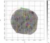 |
Fig. 1 A mosaic image of the MOS 1, MOS 2, and pn exposures in the 0.3–10 keV energy band (see text for details). |
For each of the detected sources, we derived the X-ray flux (in units of erg s-1 cm-2) in a given band as  (1)where Bi is the count rate in the i band and ECFi is an energy conversion factor which has been calculated using the most recent calibration matrices for the MOS 1, MOS 2, and pn. ECFs for each camera, energy band, and filter are in units of 1011 counts cm2 erg-1. In particular, we used the ECFs4 obtained assuming a power-law model with photon index Γ = 1.7 and a Galactic foreground absorption of NH ≃ 3.0 × 1020 cm-2 (Watson et al. 2009). Note also that the adopted hydrogen column density is of the same order of magnitude as the average value estimated towards the target by using the “NH” online calculator5, i.e., 2.7 × 1020 cm-2 (Kalberla et al. 2005).
We refined the absolute astrometry by matching the candidate source lists to the USNO-B1 catalog (Monet et al. 2006). From this catalog, we extracted a sub-sample of stars with coordinates within 20′ from the Fornax center and used the SAS task eposcorr (with parameter of maximum distance of 1″) to obtain the coordinate correction which was (on average) − 0.56″ ± 0.50″ in RA and − 1.77″ ± 0.34″ in Dec. We purged the candidate source lists (one per EPIC camera) by accepting only sources with a maximum likelihood detection (as provided by the source detection algorithm) larger than 10 (equivalent to 4σ) and then cross correlated the source lists via the IDL routine srcor.pro6 by requiring a critical radius of 1″ outside which the correlations were rejected and obtained the source parameters (i.e., coordinates, count rates, fluxes, and hardness ratios) by weighting (with the errors) the values of interest associated with the sources identified in the three cameras.
After removing a few spurious sources (i.e., those positioned at the borders of the cameras and those not appearing as such in the 0.2–12 kev band), our catalog resulted in 107 sources detected towards the Fornax dSph galaxy with, in particular, 32 sources identified contemporarily in MOS 1, MOS 2, and pn, 4 sources only in MOS 1 and MOS 2, 7 sources only in MOS 1 and pn, 18 sources only in MOS 2 and pn, 30 sources only in pn, 2 sources only in MOS 1, and 14 sources only in MOS 2. Note that the number of detected sources agrees very closely with the 104 sources found by Orio et al. (2010) when analyzing the same data set, the discrepancy probably arising from slightly different choices in the data screening procedure and the detection threshold used. A mosaic image (logarithmically scaled and smoothed with a 3-pixel Gaussian kernel) of the MOS 1, MOS 2, and pn exposures in the 0.3–10 keV energy band is given in Fig. 1. Here, each of the identified sources is indicated by a 35″ radius circle (containing ≅ 90% of energy at 1.5 keV in the pn camera, see e.g. the XRPS User’s Manual 2008), labeled with a sequential number and with a color depending on which camera (or set of cameras) the source was detected by: yellow (pn), magenta (pn and MOS 1), red (pn and MOS 2), black (pn, MOS 1, and MOS 2), blue (MOS 1 and MOS 2), cyan (MOS 1), and green (MOS 2). The red-dashed ellipse indicates the extension of the galaxy which is characterized by semi-major and semi-minor axes of ≃ 17′ and ≃ 13′ (see the NASA/IPAC extragalactic database7 -NED-) and a major-axis position angle of ≃ 48° (Mateo 1998b).
In Table 1 we summarize our source analysis, ordering the list by increasing X-ray flux in the 0.2–12 keV energy band. Here, we give a sequential number (Scr) for each source, a label (#) indicating which EPIC camera (or set of cameras) identified the source, i.e., A (pn only), B (pn and MOS 1), C (pn and MOS 2), D (pn, MOS 1, and MOS 2), E (MOS 1 and MOS 2), F (MOS 1), and G (MOS 2). We also give the J2000 coordinates with the associated errors (Cols. 3–5), the high-energy hardness ratios HR1 and HR2 (see next section) (Cols. 6–7), the 0.2–12 keV absorbed flux (Col. 8) and the cross correlations (Cols. 9–10).
We used the Two Micron All-Sky Survey (2MASS), the Two Micron All-Sky Survey Extended objects (2MASX; Skrutskie et al. 2006), the United States Naval Observatory all-sky survey (USNO-B1; Monet et al. 2006), and the variable star catalog in the Fornax galaxy (Bersier & Wood 2002) to correlate the X-ray source catalog with optical counterparts. In doing this, we associated with the coordinates of each of the identified X-ray source an error as resulting from the quadrature sum of the XMM-Newton positional accuracy ( ≃ 2″ at 2σ confidence level, see Kirsch 2004, and Guainazzi 2010) and the statistical error as determined by the edetectchain tool8. Similarly, the error associated with the optical counterpart was derived from the relevant catalog.
When an X-ray source is found to be within 1σ from an optical counterpart in a given catalog, we report in Table 1 the corresponding distance in arcseconds in the relevant column. We remind the reader that the Fornax dSph galaxy was already the target of a ROSAT X-ray observation (see Gizis et al. 1993, for details) with the purpose of characterizing the X-ray population (if any) in the galaxy and of constraining the extended gas component. The analysis of the ROSAT data resulted in the compilation of a catalog (hereinafter GMD093) listing 19 discrete sources congruous with the expected number of sources in the extragalactic background. In Table 2 we give the GMD093 labels and coordinates (Cols. 1–3) of the sources observed by ROSAT and the labels of the corresponding sources in our catalog (Col. 4). The distance between the sources in the GMD093 catalog and the corresponding sources found in the XMM-Newton list is given in the fifth column with the error evaluated as the sum in quadrature between the XMM-Newton and ROSAT positional accuracies9. Finally, a possible classification (based on the SIMBAD10 and NED web sites) is attempted in the sixth column (QSO -quasar-, EmG -emission line galaxy-, H2G -HII galaxy-, SyG -Seyfert galaxy-): when a source is not cross correlated with SIMBAD and/or NED, this is simply labeled as Xrs (X-ray source). Note that, among the 19 sources belonging to the GMD093 catalog, 6 are out of the XMM-Newton field of view. Furthermore, from the LX-LB relation (LB being the Fornax dSph B band luminosity), Gizis et al. (1993) estimated that at least one accreting binary should be present in the field of view. For completeness, we mention that as far as the extended component is concerned, the ROSAT data did not show any diffuse emission different from the normal X-ray background and no trend with radius was evident. Here, we concentrate on the point-like sources identified in the XMM-Newton observation of the Fornax dSph.
The X-ray sources detected by our analysis towards the Fornax dSph.
List of the detected X-ray sources cross-correlated with the catalog GMD093 (Gizis et al. 1993).
3. The high-energy view of the Fornax dSph
3.1. X-ray colors and X-ray-to-NIR flux ratios
Using the results presented in the previous section and with the purpose of a tentative classification of all the sources identified towards the Fornax dSph, we constructed the color–color diagram in Fig. 2. Here, we considered the colors  (2)following the convention used in Ramsay & Wu (2006) in studying the Sagittarius and Carina dwarf galaxies and first introduced by Prestwich et al. (2003) and Soria & Wu (2003) S, M, and H correspond to the count rates in 0.3–1 keV, 1–4 keV, and 4 − 10 keV energy bands.
Since we expect that the detected X-ray sources are mainly accreting compact objects such as background active galactic nuclei (AGN), X-ray binaries, and the brighter end of cataclysmic variables (CVs), we compared the source measured hardness ratios (red squares) with two spectral models (power-law, for simulating AGN and X-ray binaries, and bremsstrahlung, for CVs) which may be used to have an overall, although simplified, description of the source spectra (see e.g. Ramsay & Wu 2006, for a similar analysis made on the Sgr and Car dSphs). The model tracks, appearing in the color–color diagram, were obtained by simulating synthetic spectra within XSPEC (An X-Ray Spectral Fitting Package, Arnaud 1992), version 12.0.0. In particular, we give the expected set of color–color contours for bremsstrahlung (grey region) and power-law (black region) components. In both cases, the equivalent hydrogen column density NH varies in the range 1019 cm-2 to 1022 cm-2: each of the almost horizontal lines corresponds to models with equal NH which increases from bottom to top. The temperature kT of the bremsstrahlung models (taken in the range 0.1–3 keV) and the power-law index Γ (in the range 0.1–3) is associated with primarily vertical lines: the values of kT and Γ increase from left to right and from right to left, respectively. A representative error bar, obtained by averaging all the data point error bars, is also given. Most of the detected sources have colors consistent with those of the absorbed power-law or absorbed bremsstrahlung models, although a few of them may require combined spectra.
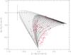 |
Fig. 2 Color–color diagram of the sources detected by the EPIC cameras towards the Fornax dSph galaxy. The solid lines represent the theoretical tracks expected for different emitting models (see text for details). A representative error bar (obtained averaging all data point error bars) is also shown. |
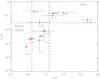 |
Fig. 3 Color–color diagram for the X-ray sources of our sample with a counterpart in the 2MASS catalog (see text for details). |
Most of the sources appear to have spectra consistent with that of a typical AGN (which in the hardness diagram of Fig. 2 would correspond to a dot lying close to the harder color–color tracks, see e.g. Ramsay & Wu 2006). However, because the large error bars affect the hardness ratio data, a classification based only on the hardness ratio cannot constrain the nature of the objects in our sample.
A better diagnostic tool was found by Haakonsen & Rutledge (2009) when studying the cross associations of the ROSAT All-Sky Survey Bright Source Catalog (RASS/BSC) with the infrared counterparts found in 2MASS. In particular, these authors found that a color–color diagram (based on the ratio between the 0.2–2.4 keV flux (FX) and the NIR flux in J band (FJ) versus the J − K color) is useful in studying the characteristics of the sources. In this plane, the galaxies (Quasars and Seyfert 1 objects) and the coronally active stars (including pre-main sequence and main-sequence stars, high proper-motion objects, and binary stars) occupy distinct regions in such a way that galaxies have (J − K) > 0.6 and FX/FJ > 3 × 10⁻² (dashed red lines in Fig. 3), while almost all the objects in the second class have (J − K) < 1.1 (dotted black line in Fig. 3) and FX/FJ < 3 × 10⁻², respectively11. For the sources of our sample which correlate with 2MASS counterparts, we give in Table 3 the 0.2 − 2.4 keV band flux, the NIR J band flux and the J and K magnitudes. Note that the 0.2 − 2.4 keV band flux has been obtained from that in the 0.2–12 keV band (given in Table 1) assuming in webPIMMS a power-law model with a spectral index Γ = 1.7 and an absorption column density NH = 3 × 1020 cm-2. In Fig. 3, we give the color–color diagram (X-ray to J band flux ratio against J − K) for the sources listed in Table 3. The sources lying above the horizontal dashed line are consistent with background AGN, while the others seem to have characteristics similar to X-ray active stars and binary sources: three of them (19, 41, and 82) have measured proper motions in the PPMX catalog (see also Table 1), confirming the stellar nature of these objects. Note that the X-ray source labeled as 107 correlates (within 1.0″) with a source in the 2MASX and, according to our color–color diagram, is possibly associated with a background AGN (see also Mendez et al. 2011, where it is used as a reference background AGN for proper motion estimates), while it was probably reported in the PPMX catalog by mistake (source labeled as 024019.0–343719): this confirms the predictive power of this color–color diagram.
A few sources of the X-ray sample detected towards the Fornax dSph correlate with the 2MASS catalog.
3.2. Background sources from the log N – log S plot
We estimated the number of background sources expected towards the Fornax dwarf galaxy through the log N − log S diagram (Hasinger et al. 2005) and by using the minimum absorbed flux in the 0.2–12 keV band among the sources of our analysis, i.e.,  . Using webPIMMS v3.912 and assuming a power-law model with a spectral index Γ = 1.7 and an absorption column density NH = 3 × 1020 cm-2, we obtained an unabsorbed flux in the same band
  , hence
  in the 0.5–2 keV band.
We used this value as an input parameter of the Hasinger et al. (2005) method, obtaining a theoretical number of AGN as a function of the angular distance from the galactic center. Then we divided the Fornax field of view (FOV) into five rings and compared the number of sources observed in each annulus to the expected number using the log N − log S relation (Hasinger et al. 2005), see Table 4. The number of sources detected in each annulus is consistent with the expected number except in the external annulus, as the expected value does not account for border effects although all the detected sources in the Fornax FOV may be background objects, because of the intrinsic statistical meaning of the log N − log S diagram, it cannot be ruled out that some of them actually belong to the galaxy itself. This conclusion is somehow supported by Fig. 3 where the X-ray sources in the bottom-left region are most likely of local origin.
3.3. Hint of a local variable source associated with an X-ray source
When searching for optical counterparts to the detected X-ray sources (see Table 1) in the available catalogs, we found that source number 61 is possibly associated, within 2″, with one source (J023941.4-343340) belonging to a catalog of variable stars (Bersier & Wood 2002), making it a good candidate for a genuine X-ray source in the Fornax galaxy. The angular sensitivity of XMM-Newton, however, makes it difficult to separate this source from the one labeled 80 (see Fig. 1) which is only ≃ 22″ apart. One solution is to reduce the contamination from the nearby source by reducing the source extraction radius and by selecting suitable background regions. In the particular case of source 61, we used a source extraction circle with a radius of ≃11″ (corresponding to ≃50% of the source encircled energy, see XRPS User’s Manual 2008) and extracted the background from a circular region having the same radius as the source extraction area and localized at a distance of ≃22″ from source 80. The latter choice allowed us to properly remove the background noise as well as any pattern hidden in the data caused by the proximity of source 80. We then extracted the pn spectrum of source 61 (which consisted of only ≃ 200 counts) and fitted it with an absorbed power-law model with hydrogen column density fixed to the value 2.7 × 1020 cm-2 (see Sect. 2.2). The best fit, which converged to a power-law index Γ ≃ 2.0, corresponded to a flux in the 0.2–12 keV energy band of ≃ 2.0 × 10⁻¹⁴ erg s-1 cm-2 consistent with that obtained from the analysis discussed in Sect. 2 (see also Table 1).
Using the extraction regions previously described, we generated source and background pn light curves (with a bin-size of 500 s) from the cleaned event files and used the SAS task epiclccorr to account for absolute and relative corrections and for the background subtraction. The resulting light curve was then analyzed with the Lomb-Scargle method (Scargle 1982) to search for periodicities in the range 1000–10 000 s and the significance of any possible features appearing in the Lomb-Scargle periodogram was evaluated by comparing the peak height with the power threshold corresponding to a given false alarm probability in white noise simulations (Scargle 1982). When applied to the presently available data, this method did not detect any clear periodicity.
List of sources expected through the log N − log S diagram and observed in annuli around Fornax center.
3.4. The Fornax globular clusters
Among all the other dSphs which are satellites of the Milky Way, the Fornax dSph has the peculiar characteristic of hosting five globular clusters (GCs) whose (J2000) coordinates and main structural parameters (mass M, core radius rc, projected distance Rp from the galaxy center, tidal radius rt, and maximum radius rM) are reported in Table 5. Apart from the puzzling question of why dynamical friction has not yet dragged any of the Fornax GCs towards the center of the galaxy (see e.g. Cole et al. (2012) for an introduction to this intriguing problem and to Goerdt et al. 2006 for a possible solution13), a search for X-ray sources associated with the GCs is also interesting. We performed this search towards the five Fornax dSph GSs and found that a few X-ray sources are located close to GC 3 and GC 4 (see the zoomed views of the XMM-Newton field around the two clusters in Figs. 4 and 5.
For GC 4, the three green dashed concentric circles are centered on the GC coordinates and have radii of 2.6″, 43″, and 64″, corresponding to the cluster core radius, tidal radius, and maximum radius (see also Table 5) as given in Cole et al. (2012) and MacKey & Gilmore (2003). In the case of GC 3, for clarity, we have plotted only the circles having a radius equal to the core radius (2.4″) and tidal radius (77″).
Coordinates of the Fornax globular clusters are taken from the NASA/IPAC extragalactic database (NED).
All the other circles (with associated radii of 35″) appearing in the figures indicate the X-ray sources detected in our analysis (see Sect. 2.2).
In the case of GC 4, we identified one X-ray source (labeled as 28 in the source list appearing in Table 1) which is at a distance of ≃ 37″ from the globular cluster center14. Consequently, considering the GC 4 structural parameters reported in Table 5, one observes that source 28 is well within the tidal radius ( ≃ 43″) of the globular cluster and possibly associated with it, as already noted by Orio et al. (2010) when analyzing the same XMM-Newton data set.
In the case of GC 3, two variable Sx Phe sources15 (6_V40765 and 6_V38403) were identified by Poretti et al. (2008) as belonging to the globular cluster. Both sources appear to be at a distance of ≃ 30″ and ≃ 78″ from the globular cluster center and, therefore, are possibly associated with GC 3. As one can see from a close inspection of Fig. 5, there is no clear association of any of the variable stars (blue crosses) observed in GC 3 with the detected X-ray sources. Moreover, one X-ray source (labeled as 103 at ≃ 72″ from the globular cluster center) and identified in the XMM-Newton field of view is within the globular cluster tidal radius ( ≃ 77″) and, therefore, may be associated with it (as already claimed by Orio et al. 2010). Finally, we note that for an estimated distance of 0.138 Mpc to the Fornax dSph, the observed 0.2–12 keV band luminosities associated with the sources 28 and 103 are ≃ 2.3 × 1034 erg s-1 and ≃ 2.6 × 1035 erg s-1, respectively. While the source possibly associated with GC 4 has a luminosity comparable to that of a typical CV, the source possibly residing in GC3 has a luminosity well within the typical ranges (although towards the lower limit) for LMXBs and high-mass X-ray binaries (HMXBs; see e.g. Fabbiano & White 2006; Kuulkers et al. 2006; and Tauris & van den Heuvel 2006).
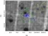 |
Fig. 4 Zoomed view of the region around the Fornax globular cluster GC 4 (see text for details). |
3.5. An intermediate-mass black hole in the Fornax galaxy: high-energy constraints
When the galactic globular clusters were identified in X-rays, Bahcall & Ostriker (1975) and Silk & Arons (1976) suggested that the observed emission was due to the presence of IMBHs in the mass range ~102 M⊙–105 M⊙ accreting material from the intracluster medium.
The discovery of ultra-luminous compact X-ray sources (ULXs, with luminosity greater than ~1039 erg s-1) initially pushed the community to interpret such objects as IMBHs. Note however that the current accepted sceario is that all the ULXs (with the exception of the highest luminosity objects still contain an IMBH) are stellar-sized black holes which accrete at super-Eddington rates (Miller & Colbert 2003). More evidence comes from the study of the central velocity dispersion of stars in specific globular clusters (as G1 in the Andromeda galaxy, see e.g. Gebhardt et al. 2002; but also Pooley et al. 2006, or M15 and ω Centauri in the Milky Way; see e.g. Gerssen et al. 2002, 2003, and Miocchi 2010, respectively) which may contain central IMBHs. As far as M15 is concerned, milli-second pulsar timing studies have allowed us to put an upper limit of ≃ 3 × 10³ M⊙ on the IMBH mass (De Paolis et al. 1996). Finally, compact objects of IMBH size are also predicted by N-body simulations (see e.g. Portegies Zwart et al. 2004) as a consequence of merging of massive stars. As noted by several authors (see e.g. Baumgardt et al. 2005; Miocchi 2007), photometric studies may provide a further hint for the existence of IMBHs in globular clusters. It is expected that the mass density profile of a stellar system with a central IMBH follows a cuspy ρ ∝ r−7/4 law, so that the projected density profile, as well as the surface brightness, should also have a cusp profile with slope −3/4.
As shown by Miocchi (2007), the globular clusters that most likely host a central IMBH are those characterized by a projected photometry well fitted by a King profile, except in the central part where a power-law deviation (α ≃ − 0.2) from a flat behavior is expected. However, the errors with which the slopes of central densities can be determined are approximately 0.1 − 0.2 (Noyola & Gebhardt 2006), so that optical surface density profiles do not give clear evidence of the existence of IMBH in globular clusters.
It is then natural to expect that observations in different bands of the electromagnetic spectrum, such as radio and X-ray bands, would permit further constraints on the IMBH parameters. This issue was considered by several authors. For example, Grindlay et al. (2001) provided the census of the compact objects and binary populations in the globular cluster 47 Tuc and obtained an upper limit to the central IMBH of a few hundred solar masses; Nucita et al. (2008) showed that the core of the globular cluster NGC 6388 harbors several X-ray sources; and Cseh et al. (2010) refined the analysis putting an upper limit to the central IMBH mass of a few thousand solar masses (see also Bozzo et al. 2011; Nucita et al. 2012).
One expects to find IMBHs in dSph as well (Maccarone et al. 2005). In the specific case of the Fornax dSph, van Wassenhove et al. (2010) assumed that an IMBH of mass MBH ≃ 105 M⊙ exists in the galactic core and suggested that measuring the dispersion velocity of the stars within 30 pc from the center would allow us to test that hypothesis. Furthermore, Jardel & Gebhardt (2012) recently constructed axisymmetric Schwarzschild models in order to estimate the mass profile of the Fornax dSph. These models were tested versus the available kinematic data allowing the authors to put a 1-σ upper limit of MBH = 3.2 × 10⁴ M⊙ on the IMBH mass. We will use the latter value in the following discussions.
Since any Brownian motion of IMBH at the center of the galaxy is negligible16, we searched for X-ray sources close to the Fornax center. This search was made difficult owing to the uncertainty with which the Fornax dSph center position is known. This is caused mainly by the large asymmetry in the galaxy surface brightness as first observed by Hodge (1961; see also Hodge & Smith 1974). The asymmetry was also confirmed by Stetson et al. (1998) who evaluated the global galaxy centroid using a circle moving on the sky plane until the median (x, y) position of all the stars contained within the aperture coincided with the center of the circle. Depending on the circle radius (500 or 2000 pixels), Stetson et al. (1998) obtained two center positions (separated by ≃ 3′) indicated by the green diamonds (with labels SHS98 500 pxl and SHS98 2000 pxl) in Fig. 6. In the same figure, we also give the coordinates of the centroid as obtained by Hodge & Smith (1974; red diamond) and Demers & Irwin (1987; black diamond). For comparison, the yellow diamond (on a CCD gap of the pn camera) represents the centroid as recently determined by Battaglia et al. (2006) and the blue diamond is centered on the NED coordinates of Fornax dSph.
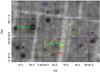 |
Fig. 6 Zoomed view around the Fornax dSph center. The diamonds indicate the global centroids of the galaxy obtained by several authors. In particular, the green diamonds (with labels SHS98 500 pxl and SHS98 2000 pxl) correspond to the galaxy centers obtained by Stetson et al. (1998), the red and black diamonds indicate the centroids as derived by Hodge & Smith (1974) and Demers & Irwin (1987), respectively (see text for details). |
Note that the centroid labeled SHS98 2000 pxl, as estimated by Stetson et al. (1998) when considering the large structure of the galaxy, is at a distance of ≃ 28″ from the centroid position according to Battaglia et al. (2006) and is apparently very close to one of the X-ray sources (labeled 2) detected in our analysis, thus allowing us to estimate the X-ray luminosity from a putative IMBH. In all the other cases, the centroids fall in a region apparently free of sources, so that only an upper limit on the IMBH flux can be obtained. As a reference for this case we use SHS98 500 pxl as the position of the centroid.
In the following paragraphs we speculate about the possible existence of an IMBH in the Fornax dSph and whether it is in the position labeled SHS98 2000 pxl or coincident with the centroid SHS98 500 pxl.
As in the case of the G1 (Pooley & Rappaport 2006) and M15 (Ho et al. 2003) globular clusters, the X-ray emission from the putative IMBH at the center of the Fornax dSph may be due to Bondi accretion (Bondi & Hoyle 1994) onto the black hole, either from the cluster gas or from stellar winds. Thus, assuming that low-angular momentum gas close to the compact object accretes spherically, for a black hole of mass MBH moving with velocity v through a gaseous medium with hydrogen number density n, the accretion rate is 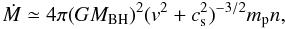 (3)where mp and cs are the proton mass and sound speed in the medium, respectively. The expected X-ray luminosity is then
  (4)which can be parametrized as
  (5)where
  , ϵ is the efficiency in converting mass to radiant energy and η is the fraction of the Bondi-Hoyle accretion rate onto the black hole.
The hydrogen number density of the mass feeding the black hole can be estimated by using the structural parameters of the Fornax dSph as given in McConnachie (2002). In particular, it was found that the galaxy hosts at least MHI ≃ 0.17 × 10⁶ M⊙ of gas within the observed half-light radius of rh ≃ 710 pc. Thus, a lower limit to the gas density can be evaluated as  (6)Assuming that v ≃ cs ≃ 10 km s-1, one has V ≃ 14 − 15 km s-1. Thus, using the IMBH upper limit of MBH = 3.2 × 10⁴ M⊙ quoted above, Eq. (5) finally gives the expected X-ray luminosity, i.e.,
  (7)For an estimated distance of 0.138 Mpc to the Fornax dSph, the expected IMBH luminosity LX corresponds to an observable flux of FX ≃ ϵη1.98 × 10⁻¹⁰ erg s-1 cm-2.
As one can see from a close inspection of Fig. 6, in the case when the putative IMBH position coincides with the centroid SHS98 500 pxl17, there was no clear detection of X-ray counterparts in the 0.2–12 keV band. To be conservative, the expected flux can be compared with the minimum (unabsorbed) flux ( ≃ 2.5 × 10⁻¹⁵ erg s-1 cm-2, see Sect. 2.4 for further details) detectable in the XMM-Newton observation. Hence, one easily constrains the accretion efficiency of the IMBH to be ϵη ≤ 1.3 × 10⁻⁵.
On the contrary, a detection appears (source labeled 2) on the centroid SHS98 2000 pxl position. In this case, using the flux values obtained by the automatic procedure described in Sect. 2, we found that source 2 has an unabsorbed flux (obtained via webPIMMS) in the 0.2–12 keV of ≃ 3.0 × 10⁻¹⁵ erg s-1 cm-2 which, at the Fornax dSph distance, corresponds to an intrinsic luminosity of LX = 7.0 × 1033 erg s-1. Thus, in the IMBH hypothesis, the accretion efficiency turns out to be ϵη ≃ 1.6 × 10⁻⁵.
With a more detailed analysis, we further extracted the MOS 1, MOS 2, and pn spectra of source 2 using a circular region centered on the target coordinates and with radius of 35″. We then accumulated the background on a region located on the same chip and in a position apparently free of sources. This resulted in MOS 1, MOS 2, and pn spectra with ≃ 230, ≃ 250, and ≃ 480 counts, respectively.
After grouping the data by 25 counts/bin, we imported the resulting background-reduced spectrum within XSPEC. A model consisting of an absorbed power-law, with hydrogen column density fixed to the average value observed towards the target (2.7 × 1020 cm-2, see Sect. 2 for further details), resulted in the best fit parameters  and N = (5.0 ± 4.0) × 10-7 kev-1 cm-2 s-1 with
  (for 34 d.o.f.). The 0.2 − 12 keV band absorbed flux of source 2 is then
  erg s-1 cm-2 (90% confidence level) which corresponds to an unabsorbed flux of ≃ 6.2 × 10⁻¹⁵ erg s-1 cm-2 and an unabsorbed luminosity of LX ≃ 1.4 × 1034 erg s-1. Assuming a spherical accretion, one finally has an accretion efficiency of ϵη ≃ 3 × 10⁻⁵.
Note also that for η = 1, the radiative efficiency ϵ of the putative Fornax dSph IMBH is similar to the values found for other systems in the radiatively inefficient regime (10-5–1, see Baganoff et al. 2003; but also Fender et al. 2003, and Koerding et al. 2006a,b). The same conclusion can be reached when comparing the observed X-ray luminosity in the 0.2–12 keV band of source 2 (LX ≃ 1.4 × 1034 erg s-1) with the expected Eddington luminosity (i.e., LEdd ≃ 1.3 × 1038(MBH/M⊙) erg s-1) in the IMBH hypothesis. In this case, LX/LEdd ≃ 3 × 10⁻⁹ is obtained, thus implying that the IMBH must be extremely radiatively inefficient (for a comparison see the M15 case discussed in Ho et al. 2003). Accretion onto a black hole may be different from a simple spherical model, since the accreting gas has angular momentum. In such a case a Keplerian disk forms and the accretion occurs due to the presence of viscous torques, which transport the angular momentum outward from the inner to the outer regions of the disk (see e.g. Shapiro & Teukolsky 1983). In the simplified case of a thin disk structure (see Shakura & Sunyaev 1973), the total luminosity of the disk (mainly originating in its innermost parts) is  (8)where Ṁ is the accretion rate and rI is the radius of the inner edge of the disk. For a disk that extends inward to the last stable orbit (rI = 6GMBH/c2 for a non-rotating black hole), it is easy to verify that the efficiency in converting the accreting mass to radiant energy is ≃ 8.3%. When comparing the observed X-ray luminosity in the 0.2–12 keV band of source 2 with the value expected in the thin disk scenario (Eq. (8)), we can estimate a mass accretion rate of Ṁ ≃ 1.87 × 10¹⁴ g s-1. Assuming again the radiation efficiency to be 8.3%, a black hole of mass 3.2 × 10⁴ M⊙ has an Eddington mass accretion rate of ṀEdd ≃ 5.5 × 10²² g s-1. Thus, the ratio Ṁ/ṀEdd ≃ 4 × 10⁻⁹ implies that the IMBH in Fornax dSph (if any) accretes very inefficiently even in the context of a Keplerian thin disk model.
The above considerations, the observed low luminosity, and the estimated power-law index (marginally consistent with an index in the range 1.4–2.1, see e.g. Remillard & McClintock 2006, for a classification of black hole binaries) allow us to depict a scenario in which the Fornax dSph IMBH may be in a quiescent state.
Recently, it has also been proposed that a relationship between black hole mass, X-ray luminosity, and radio luminosity does exist (see e.g. Merloni et al. 2003; Koerding et al. 2006a). This fundamental plane can be used to test the IMBH hypothesis in globular clusters and dwarf spheroidal galaxies (Maccarone et al. 2005). In particular, Maccarone (2004) scaled the fundamental-plane relation to values appropriate for an IMBH host in a Galactic globular cluster; by rescaling their equation to estimate the expected IMBH radio flux at 5 GHz, i.e.,  (9)which, for the above X-ray flux estimates, corresponds to
  (10)For an accretion efficiency as low as a few 10-5, the expected radio flux is well within the detection possibilities of the Australia Telescope Compact Array (ATCA) which, for an integration time of ≃ 12 h, may reach an RMS sensitivity of ≃ 10 μJy/beam at 5 GHz.
4. Conclusions
In this paper we re-analyzed a deep archive XMM-Newton data of the Fornax dSph galaxy with the aim of characterizing the X-ray point-like source population. By using a restrictive analysis, we detected 107 X-ray sources. Most of them are likely to be background objects since the number of detected sources is statistically consistent with that expected from the log N − log S relation. However, we cannot exclude that a few of the detected objects belong to the Fornax dSph. The color–color diagram (based on the ratio between the 0.2–2.4 keV flux (FX) and the NIR flux in J band (FJ) versus the J − K color) for the X-ray sources with a counterpart in the 2MASS catalog shows the presence of a few objects (see bottom-left part of Fig. 3) possibly of stellar nature and local origin. Furthermore, source number 61 appears to be spatially coincident (within ≃ 2″) with a long-period variable star found in the catalog compiled by Bersier & Wood (2002).
As discussed previously, among all the other dwarf spheroidal satellites of the Milky Way, a peculiar characteristic of the Fornax dSph is that of hosting five globular clusters. We noted that two X-ray sources, detected towards the galaxy with our analysis, are coincident with the two Fornax globular clusters GC 3 and GC 4. In particular, for GC 4 we identified one X-ray source (labeled 28 in the source list appearing in Table 1) which is at a distance of ≃ 37″ from the globular cluster center. Consequently, considering the GC 4 structural parameters reported in Table 5, one observes that source 28 is well within the tidal radius ( ≃ 43″) of the globular cluster and, hence, possibly associated with it (as already claimed by Orio et al. 2010). In the case of GC 3, we identified one X-ray source (labeled 103 at a distance of ≃ 72″ from the GC center) that might be at the outskirts of the globular cluster.
Finally, we discussed the IMBH hypothesis and found that one of the X-ray sources (labeled 2) might be associated with one of the possible galaxy centroids identified by Stetson et al. (1998). In this framework, we estimated the IMBH accretion parameter to be ϵη ≃ 10-5. However, since there is a large uncertainty in the identification of the galaxy’s center of gravity, the latter value can be considered as an upper limit to the IMBH accretion parameters.
For more details, the reader is addressed to the on-line thread: http://xmm.esac.esa.int/sas/current/documentation
For details on the adopted ECFs, see Saxton (2003). Please note that, since 2008, improvements in the calibration of EPIC cameras lead to changes in the ECFs. Thus, the quoted ECFs must be multiplied by a correction factor to get a better agreement among the fluxes evaluated in each camera (Stuhlinger et al. 2006). The ECFs and associated correction factors are reported in the User’s Guide of the 2XMM catalog of serendipitous sources available at http://xmmssc-www.star.le.ac.uk/Catalogue/2XMMi-DR3.
Available in the tool section of http://heasarc.nasa.gov
Since the resulting positional uncertainty is of a few arcseconds, we do not over-plot the source error circles in any of the figures appearing in the paper.
Because of the lack of any positional uncertainty on the sources reported in Gizis et al. (1993), we associated each of the ROSAT detected sources with an error of ≃ 15″ on both the celestial coordinates: we are aware that this error may be underestimated since the positional accuracy of ROSAT PSPC decreases with increasing offset from the detector axis.
Note that a better diagnostic would use the unabsorbed X-ray flux in the 0.2–2.4 keV band and the extinction-corrected NIR magnitudes: in the proposed color–color diagram of Haakonsen & Rutledge (2009), the galaxies are positioned in the region described by (J − K) > (J − K)0 > 0.6 and (FX/FJ)0 > FX/FJ > 3 × 10⁻². On the contrary, the coronally active stars satisfy the relations (J − K)0 < (J − K) < 1.1 and (FX/FJ) < (FX/FJ)0 < 3 × 10⁻², with the subscript 0 indicating the result of the de-reddening procedure (see Haakonsen & Rutledge 2009, for details).
Goerdt et al. (2006) have shown that dynamical friction cannot drag globular clusters to the galaxy center in the case of cored dark-matter halo distributions. In this case the drag is stopped at the point where the dark-matter density remains constant, i.e., ≃ 200 pc.
We checked that none of the X-ray sources of our sample has a counterpart in the catalog of variable stars (indicated as blue crosses in Fig. 4) as reported by Greco et al. (2007).
A Sx Phe object is a variable pulsating star whose magnitude can vary from a few 0.001 mag to several 0.1 mag with typical periods of P ≲ 0.10 days and is often used as a distance estimator. For a description on the main properties of this class of variable stars we refer the reader to Pych et al. (2001) and references therein.
From simulations, one expects an IMBH within a globular cluster (or a spheroidal galaxy) to move randomly when interacting with the surrounding stars. In the assumption that all the stars have the same mass m, the IMBH moves with an amplitude ~ rc(m/MBH) (see e.g. Bahcall & Wolf 1976; Gurzadyan 1982; Merritt et al. 2006) where rc is the core radius and MBH the black hole mass.
In the case in which the Fornax centroid position coincides with one of those evaluated by Hodge & Smith (1974), Demers & Irwin (1987), or Battaglia et al. (2006) (red, black, and yellow diamonds in Fig. 6, respectively), we can set only an upper limit to the IMBH unabsorbed flux of ≃ 2.5 × 10⁻¹⁵ erg s-1 cm-2 which, at the distance of the Fornax dSph, corresponds to a luminosity limit of ≃ 5.7 × 1033 erg s-1.
Acknowledgments
We are grateful to F. Strafella, V. Orofino, and B.M.T. Maiolo for the interesting discussions while preparing the manuscript. We also acknowledge the anonymous Referee for his suggestions.
References
- Arnaud, K. A. 1996, XSPEC: The First Ten Years, in Astronomical Data Analysis Software and Systems V, eds. G. Jacoby, & J. Barnes (San Francisco: ASP) ASP Conf. Ser., 101, 17 [Google Scholar]
- Ashman, K. M., & Zepf, S. E. 1998, Globular Cluster Systems (Cambridge: Cambridge Univ. Press) [Google Scholar]
- Baganoff, F. K., Maeda, Y., Morris, M., et al. 2003, ApJ, 591, 891 [NASA ADS] [CrossRef] [Google Scholar]
- Bahcall, J. N., & Ostriker, J. P. 1975, Nature, 256, 23 [NASA ADS] [CrossRef] [Google Scholar]
- Bahcall, J. N., & Wolf, R. A. 1976, ApJ, 209, 214 [NASA ADS] [CrossRef] [Google Scholar]
- Battaglia, G., Tolstoy, E., Helmi, A., et al. 2006, A&A, 459, 423 [NASA ADS] [CrossRef] [EDP Sciences] [Google Scholar]
- Baumgardt, H., et al. 2005, ApJ, 589, 25 [Google Scholar]
- Bersier, D., & Wood, P. R. 2002, AJ, 123, 840 [NASA ADS] [CrossRef] [Google Scholar]
- Bondi, H., & Hoyle, F. 1944, MNRAS, 104, 273 [NASA ADS] [CrossRef] [Google Scholar]
- Bozzo, E., Ferrigno, C., Stevens, J., et al. 2011, A&A, 535, L1 [NASA ADS] [CrossRef] [EDP Sciences] [Google Scholar]
- Cole, D. R., Dehnen, W., Read, J. I., & Wilkinson, M. I. 2012, MNRAS, 426, 601 [Google Scholar]
- Cseh, D., Kaaret, P., Corbel, S., et al. 2010, MNRAS, 406, 1049 [NASA ADS] [Google Scholar]
- Demers, S., & Irwin, M. J. 1987, MNRAS, 226, 943 [NASA ADS] [Google Scholar]
- De Paolis, F., Gurzadyan, V. G., & Ingrosso, G. 1996, A&A, 315, 396 [NASA ADS] [Google Scholar]
- Ebisuzaki, T., Makino, J., Tsuru, T. G., et al. 2001, ApJ, 562, L19 [NASA ADS] [CrossRef] [Google Scholar]
- Fabbiano, G., & White, N. E. 2006, in Compact Stellar X-ray Sources, eds. W. H. G. Lewin, & M. van der Klis (Cambridge: Cambridge Univ. Press), 475 [Google Scholar]
- Farrell, S. A., Webb, N. A., Barret, D., Godet, O., & Rodrigues, J. M. 2009, Nature, 460, 73 [NASA ADS] [CrossRef] [PubMed] [Google Scholar]
- Farrell, S. A., Servillat, M., Pforr, J., et al. 2012, ApJ, 747, L13 [NASA ADS] [CrossRef] [Google Scholar]
- Fender, R. P., Gallo, E., & Jonker, P. G. 2003, MNRAS, 343, 99 [Google Scholar]
- Gebhardt, K., Rich, R. M., & Ho, L. C. 2002, ApJ, 578, L41 [NASA ADS] [CrossRef] [Google Scholar]
- Gerssen, J., van der Marel, R. P., Gebhardt, K., et al. 2002, AJ, 124, 3720 [Google Scholar]
- Gerssen, J., van der Marel, R. P., Gebhardt, K., et al. 2003, AJ, 125, 376 [NASA ADS] [CrossRef] [Google Scholar]
- Gizis, J. E., Mould, J. R., & Djorgovski, S. 1993, PASP, 105, 871 [NASA ADS] [CrossRef] [Google Scholar]
- Goerdt, T., Moore, B., Read, J. I., et al. 2006, MNRAS, 368, 1073 [NASA ADS] [CrossRef] [Google Scholar]
- Greco, C., Clementini, G., Catelan, M., et al. 2007, ApJ, 670, 332 [NASA ADS] [CrossRef] [Google Scholar]
- Grindlay, J. E., Heinke, C., Edmonds, P. D., et al. 2001, Science, 292, 2290 [NASA ADS] [CrossRef] [PubMed] [Google Scholar]
- Guainazzi, M. 2010, XMM-SOC-CAL-TN-0018, XMM-Newton Science Operations Centres, http://xmm2.esac.esa.int/docs/documents/CAL-TN-0018.ps.gz [Google Scholar]
- Gurzadyan, V. G. 1982, A&A, 114, 71 [NASA ADS] [Google Scholar]
- Haakonsen, C. B., & Rutledge, R. E. 2009, ApJS, 184, 138 [NASA ADS] [CrossRef] [Google Scholar]
- Hasinger, G., Miyaji, T., & Schmidt, M. 2005, A&A, 441, 417 [NASA ADS] [CrossRef] [EDP Sciences] [Google Scholar]
- Ho, L. C., Terashima, Y., & Okajima, T. 2003, ApJ, 587, 35 [Google Scholar]
- Hodge, P. W. 1961, AJ, 66, 249 [NASA ADS] [CrossRef] [Google Scholar]
- Hodge, P. W., & Smith, D. W. 1974, ApJ, 188, 19 [NASA ADS] [CrossRef] [Google Scholar]
- Jardel, J. R., & Gebhardt, K. 2012, ApJ, 746, 89 [NASA ADS] [CrossRef] [Google Scholar]
- Jones, D. H., Peterson, B. A., Colless, M., & Saunders, W. 2006, MNRAS, 369, 25 [NASA ADS] [CrossRef] [Google Scholar]
- Kalberla, P. M. W., Burton, W. B., Hartmann, D., et al. 2005, A&A, 440, 775 [NASA ADS] [CrossRef] [EDP Sciences] [Google Scholar]
- Kirsch, M. G. F., Altieri, B., Chen, B., et al. 2004, in Proc. SPIE, 5488, 103 [Google Scholar]
- Kleyna, J. T., Wilkinson, M. I., Evans, N. W., & Gilmore, G. 2001, ApJ, 563, L115 [NASA ADS] [CrossRef] [Google Scholar]
- Kleyna, J. T., Wilkinson, M. I., Evans, N. W., & Gilmore, G. 2002, MNRAS, 330, 792 [NASA ADS] [CrossRef] [Google Scholar]
- Koerding, E., Falcke, H., & Corbel, S. 2006a, A&A, 456, 439 [NASA ADS] [CrossRef] [EDP Sciences] [Google Scholar]
- Koerding, E. G., Fender, R. P., & Migliari, S. 2006b, A&A, 456, 439 [NASA ADS] [CrossRef] [EDP Sciences] [Google Scholar]
- Kormendy, J. 1985, ApJ, 295, 73 [NASA ADS] [CrossRef] [Google Scholar]
- Kuulkers, E., Norton, A., Schwope, A., & Warner, B. 2006, in Compact Stellar X-ray Sources, eds. W. H. G. Lewin, & M. van der Klis (Cambridge: Cambridge Univ. Press), 421 [Google Scholar]
- Maccarone, T. J. 2004, MNRAS, 351, 1049 [NASA ADS] [CrossRef] [Google Scholar]
- Maccarone, T. J. 2005, MNRAS, 364, L61 [NASA ADS] [CrossRef] [Google Scholar]
- Maccarone, T. J., Fender, R. P., Tzioumis, A. K., et al. 2005, Astrophys. Space Sci., 300, 239 [NASA ADS] [CrossRef] [Google Scholar]
- Mackey, A. D., & Gilmore, G. F. 2003, MNRAS, 340, 175 [NASA ADS] [CrossRef] [Google Scholar]
- Magorrian, J., Tremaine, S., Richstone, D., et al. 1998, AJ, 115, 2285 [NASA ADS] [CrossRef] [Google Scholar]
- Martin, N. F, de Jong, J. T. A., & Rix, H.-W. 2008, ApJ, 684, 1075 [NASA ADS] [CrossRef] [Google Scholar]
- Mashchenko, S., Sills, A., & Couchman, H. M. 2006, ApJ, 252, 269 [Google Scholar]
- Mateo, M. 1997, in The Nature of Elliptical Galaxies, Astron. Soc. Pac., San Francisco, eds. M. Arnaboldi, et al., ASP Conf. Ser. 116 [Google Scholar]
- Mateo, M. 1998a, in The Magellanic Clouds and Other Dwarf Galaxies, Shaker Verlag, Aachen, 53, eds. T., Richtler, & J. M., Braun, Proc. Bonn/Bochum-Graduiertenkolleg Workshop, 259 [Google Scholar]
- Mateo, M. 1998b, ARA&A, 36, 435 [NASA ADS] [CrossRef] [Google Scholar]
- McConnachie, A.W. 2012, AJ, 144, 1 [CrossRef] [Google Scholar]
- Mendez, R., et al. 2011, AJ, 143, 93 [NASA ADS] [CrossRef] [Google Scholar]
- Merloni, A., Heinz, S., & Di Matteo, T. 2003, MNRAS, 345, 1057 [NASA ADS] [CrossRef] [Google Scholar]
- Merritt, D., Berczik, P., & Laun, F. 2006, AJ, 133, 533 [Google Scholar]
- Miller, M. C., & Colbert, E. 2003, IJMP D, 13, 1 [NASA ADS] [Google Scholar]
- Miocchi, P. 2007, MNRAS, 381, 10 [NASA ADS] [CrossRef] [Google Scholar]
- Miocchi, P. 2010, A&A, 514, A52 [NASA ADS] [CrossRef] [EDP Sciences] [Google Scholar]
- Monet, D. G., Levine, S. E., Canzian, B., et al. 2003, AJ, 125, 984 [NASA ADS] [CrossRef] [Google Scholar]
- Noyola, E., & Gebhardt, K. 2006, AJ, 132, 447 [NASA ADS] [CrossRef] [Google Scholar]
- Nucita, A. A., de Paolis, F., Ingrosso, G., et al. 2008, A&A, 478, 763 [NASA ADS] [CrossRef] [EDP Sciences] [Google Scholar]
- Nucita, A. A., De Paolis, F., Saxton, S., & Read, A. M. 2012, New Astron., 17, 589 [NASA ADS] [CrossRef] [Google Scholar]
- Orio, M., Gallagher, J., Greco, C., et al. 2010, AIP Conf. Proc., 1314, 337 [NASA ADS] [CrossRef] [Google Scholar]
- Pooley, D., & Rappaport, S. 2006, ApJ, 644, L45 [NASA ADS] [CrossRef] [Google Scholar]
- Poretti, E., Clementini, G., Held, E. V., et al. 2008, ApJ, 685, 947 [NASA ADS] [CrossRef] [Google Scholar]
- Portegies Zwart, S. F., Baumgardt, H., Hut, P., et al. 2004, Nature, 428, 724 [NASA ADS] [CrossRef] [PubMed] [Google Scholar]
- Prestwich, A., Irwin, J. A., Kilgard, R. E., et al. 2003, ApJ, 595, 719 [NASA ADS] [CrossRef] [Google Scholar]
- Pych, W., Kaluzny, J., Krzeminski, W., et al. 2001, A&A, 367, 148 [NASA ADS] [CrossRef] [EDP Sciences] [Google Scholar]
- Ramsay, G., & Wu, K. 2006, A&A, 459, 777 [NASA ADS] [CrossRef] [EDP Sciences] [Google Scholar]
- Reines, A. E., Sivakoff, G. R., Johnson, K. E., & Brogan, C. L. 2011, Nature, 470, 66 [NASA ADS] [CrossRef] [Google Scholar]
- Remillard, R. A., & McClintock, J. E. 2006, ARA&A, 44, 49 [NASA ADS] [CrossRef] [Google Scholar]
- Roeser, S., Schilbach, E., Schwan, H., et al. 2008, A&A, 488, 401 [NASA ADS] [CrossRef] [EDP Sciences] [Google Scholar]
- Salucci, P., Wilkinson, M. I., Walker, M. G., et al. 2012, MNRAS 420, 2034 [Google Scholar]
- Saxton, R. 2003, XMM-SOC-CAL-TN-0023, version 2.0 [Google Scholar]
- Scargle, J. D. 1982, ApJ, 263, 835 [NASA ADS] [CrossRef] [Google Scholar]
- Servillat, M., Farrell, S. A., Lin, D., et al. 2011, ApJ, 743, 6 [NASA ADS] [CrossRef] [Google Scholar]
- Shakura, N. I., & Sunyaev, R. A. 1973, A&A, 24, 337 [NASA ADS] [Google Scholar]
- Shapiro, S. L., & Teukolsky, S. A. 1983, Black Holes, White Dwarfs and Neutron Stars: the physics of compact objects (New York: John Wiley & Sons) [Google Scholar]
- Silk, J., & Arons, J. 1975, ApJ, 200, L131 [NASA ADS] [CrossRef] [Google Scholar]
- Silk, J., Wyse, R., & Shields, G. A. 1987, ApJ, 322, 59 [Google Scholar]
- Skrutskie, M. F., Cutri, R. M., Stiening, R., et al. 2006, AJ, 131, 1163 [NASA ADS] [CrossRef] [Google Scholar]
- Soria, R., & Wu, K. 2003, A&A, 410, 56 [Google Scholar]
- Stetson, P. B., Hesser, J. E., & Smecker-Hane, T. A. 1998, PASP, 110, 533 [NASA ADS] [CrossRef] [Google Scholar]
- Strüder, L., Briel, U., Dennerl, K., et al. 2001, A&A, 365, L18 [NASA ADS] [CrossRef] [EDP Sciences] [Google Scholar]
- Stuhlinger, M., et al. 2006, XMM-SOC-CAL-TN-0052, version 3.0 [Google Scholar]
- Tauris, T. M., & van den Heuvel, E. P. J. 2006, in Compact Stellar X-ray Sources, eds. W. H. G. Lewin, & M. van der Klis (Cambridge Univ. Press: Cambridge), 623 [Google Scholar]
- Tinney, C. G. 1999, MNRAS, 303, 565 [NASA ADS] [CrossRef] [Google Scholar]
- Tinney, C. G., Da Costa, G. S., & Zinnecker, H. 1997, MNRAS, 285, 111 [NASA ADS] [CrossRef] [Google Scholar]
- Turner, M. J. L., Abbey, A., Arnaud, M., et al. 2001, A&A, 365, L27 [NASA ADS] [CrossRef] [EDP Sciences] [Google Scholar]
- van der Marel, R. P. 2004, Coevolution of Black Holes and Galaxies, from the Carnegie Observatories Centennial Symposia, Published by Cambridge University Press, as part of the Carnegie Observatories Astrophysics Series, ed. L. C. Ho, 37 [Google Scholar]
- van Wassenhove, S., Volonteri, M., Walker, M. G., & Gair, J. R. 2010, MNRAS, 408, 1139 [NASA ADS] [CrossRef] [Google Scholar]
- Veron-Cetty, M. P., & Veron, P. 2006, A&A, 455, 773 [NASA ADS] [CrossRef] [EDP Sciences] [Google Scholar]
- Watson, M., Schröder, A. C., Fyfe, D., et al. 2009, A&A, 493, 339 [NASA ADS] [CrossRef] [EDP Sciences] [Google Scholar]
- Webb, N., Cseh, D., Lenc, E., et al. 2012, Science, 337, 554 [NASA ADS] [CrossRef] [Google Scholar]
- West, M. J., Côté, P., Marzke, R. O., & Jordan, A. 2004, Nature, 427, 31 [NASA ADS] [CrossRef] [PubMed] [Google Scholar]
- XRPS User’s Manual 2008, Issue 2.6, eds. M. Ehle, et al. [Google Scholar]
All Tables
List of the detected X-ray sources cross-correlated with the catalog GMD093 (Gizis et al. 1993).
A few sources of the X-ray sample detected towards the Fornax dSph correlate with the 2MASS catalog.
List of sources expected through the log N − log S diagram and observed in annuli around Fornax center.
Coordinates of the Fornax globular clusters are taken from the NASA/IPAC extragalactic database (NED).
All Figures
|
Fig. 1 A mosaic image of the MOS 1, MOS 2, and pn exposures in the 0.3–10 keV energy band (see text for details). |
| In the text | |
|
Fig. 2 Color–color diagram of the sources detected by the EPIC cameras towards the Fornax dSph galaxy. The solid lines represent the theoretical tracks expected for different emitting models (see text for details). A representative error bar (obtained averaging all data point error bars) is also shown. |
| In the text | |
|
Fig. 3 Color–color diagram for the X-ray sources of our sample with a counterpart in the 2MASS catalog (see text for details). |
| In the text | |
|
Fig. 4 Zoomed view of the region around the Fornax globular cluster GC 4 (see text for details). |
| In the text | |
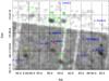 |
Fig. 5 As in Fig. 4, but the circles are centered on the coordinates of the globular cluster GC 3. |
| In the text | |
|
Fig. 6 Zoomed view around the Fornax dSph center. The diamonds indicate the global centroids of the galaxy obtained by several authors. In particular, the green diamonds (with labels SHS98 500 pxl and SHS98 2000 pxl) correspond to the galaxy centers obtained by Stetson et al. (1998), the red and black diamonds indicate the centroids as derived by Hodge & Smith (1974) and Demers & Irwin (1987), respectively (see text for details). |
| In the text | |
Current usage metrics show cumulative count of Article Views (full-text article views including HTML views, PDF and ePub downloads, according to the available data) and Abstracts Views on Vision4Press platform.
Data correspond to usage on the plateform after 2015. The current usage metrics is available 48-96 hours after online publication and is updated daily on week days.
Initial download of the metrics may take a while.