| Issue |
A&A
Volume 550, February 2013
|
|
|---|---|---|
| Article Number | A17 | |
| Number of page(s) | 7 | |
| Section | Planets and planetary systems | |
| DOI | https://doi.org/10.1051/0004-6361/201220080 | |
| Published online | 18 January 2013 | |
Exploring the nature of new main-belt comets with the 10.4 m GTC telescope: (300163) 2006 VW139
1
Instituto de Astrofísica de Canarias (IAC),
C/vía Láctea s/n, 38205
La Laguna, Tenerife
Spain
e-mail: This email address is being protected from spambots. You need JavaScript enabled to view it.
2
Departamento de Astrofísica, Universidad de La Laguna
(ULL), 38205, La
Laguna Tenerife,
Spain
3
Instituto de Astrofísica de Andalucía – CSIC,
Granada,
Spain
4
Departmento de Edafología y Geología, Universidad de La Laguna
(ULL), Tenerife,
Spain
5
INAF, Osservatorio Astronomico di Arcetri,
Italy
6
GTC Project, 38205 La Laguna, Tenerife, Spain
Received: 23 July 2012
Accepted: 20 November 2012
Abstract
Aims. We aim to study the dust ejected by main-belt comet (MBC) (300163) 2006 VW139 to obtain information on the ejection mechanism and the spectral properties of the object. This will help to see if they are compatible with those of “normal” comets.
Methods. Broad-band images in the g and r band as well as a low-resolution spectrum in the 0.35–0.9 μm region were obtained with the GTC telescope (Roque de los Muchachos Observatory, La Palma, Spain). Images were analyzed to produce a color map and derive a lower limit of the absolute magnitude H. A Monte Carlo scattering model was used to derive dust properties such as mass loss rates and ejection velocities as a function of time. The reflectance spectrum was compared to that of the well-studied MBC 133P/ Elst-Pizarro. The spectrum was also used to search for CN emission and to determine the upper limit of the CN production rate.
Results. The reflectance spectrum of 2006 VW139 is typical of a C-class asteroid, with a spectral slope S'V = 0.5 ± 1.0%/1000 Å. It is similar to the spectrum of 133P and other MBCs. No CN emission is detected in the spectrum. A CN production rate upper limit of 3.76 × 10²³ s-1 is derived. Images show that the MBC present a narrow almost linear tail that extends up to 40 000 km in the anti-solar direction and more than 80 000 km in the direction of the object’s orbital plane. The color of the tail is slightly redder than the Sun (S′ between 3−6%/1000 Å). The Monte Carlo dust tail model derived the mass loss rates and ejection velocity as a function of time, and the results show that the activity onset occurs shortly after perihelion, and lasts about 100 days; the total ejected mass is ~2 × 10⁶ kg.
Conclusions. The spectrum of 2006 VW139 suggests that it is not a “normal” comet. The spectrum is typical of the other observed MBCs. Even if no CN emission is detected, the more likely activation mechanism is water-ice sublimation. Like other well studied MBCs, (300163) 2006 VW139 is likely a primitive C-class asteroid that has a water-ice subsurface depth reservoir that has recently been exposed to sunlight or to temperatures that produce enough heat to sublime the ice.
Key words: comets: general / minor planets, asteroids: general / minor planets, asteroids: individual: (300163) 2006 VW139 / methods: observational / techniques: imaging spectroscopy
© ESO, 2013
1. Introduction
Asteroid (300163) 2006 VW139 (hereafter VW139) is the eighth main-belt asteroid observed to be “active”, i.e., with a cometary-like dust tail or coma (Hsieh et al. 2011). With a semi-major axis of a = 3.0516 AU, an eccentricity e = 0.2011, and inclination i = 3.2392°, VW139 fits into the category of main-belt comets (MBCs) following the pure phenomenological definition by Hsieh & Jewitt (2006).
Images and spectroscopy of VW139 have been presented in Hsieh et al. (2012). The authors reported that the object presents a tail aligned with the orbital plane of about 1 arcmin, and a short anti-tail of ~10′′. They claimed that this implies that the observed dust was produced by the action of a long-lived, sublimation-driven emission mechanism. They also reported that there is no evidence of any CN emission in the object spectrum and established an upper limit for the CN production rate of QCN < 1.3 × 1024 s-1.
Dynamical simulations show that MBCs are extremely unlikely to originate in the place where comets came from: the trans-Neptunian belt (TNB) and the Oort Cloud (e.g., Fernández et al. 2002). They likely formed in situ. This is the case for VW139 (Hsieh et al. 2012), which could also be a member of an asteroid collisional family (Novakovic et al. 2012). A recent work suggests that some icy trans-Neptunian objects (TNOs) might have been delivered to the asteroid belt during the Late Heavy Bombardment (Levison et al. 2009), but even those simulations fail to produce low-inclination, low-eccentricity orbits such as those of MBCs.
The asteroid 133P/Elst-Pizarro is the first discovered MBC (Elst et al. 1996) and so far the best characterized. It has been observed to be active at every perihelion passage around the orbital quadrant following perihelion, and to be inactive in the two quadrants around aphelion (Boehnardt et al. 1997; Toth 2006; Hsieh et al. 2006; 2009; 1010; Bagnulo et al. 2010). This recurring activity supports the hypothesis that 133P has an ice reservoir, which periodically sublimates and elevates dusty material into the coma and tail region. The existence of ice in MBCs is surprising, as they are close to the Sun, but recent thermal models suggest that water ice can survive at greater subsurface depth, even in the asteroid belt (Schorghofer 2008).
The MBCs 133P and 176P/LINEAR are members of the Themis collisional family. These two MBCs share surface properties with other Themis family asteroids (see Licandro et al. 2007; 2011) which indicates that they have formed in situ. Water ice has recently been discovered on the surface of (24) Themis (Campins et al. 2010; Rivkin & Emery 2010) and (65) Cybele (Licandro et al. 2011). Water ice on the surface of (24) Themis likely comes from the interior, which supports the hypothesis that there is a water ice reservoir below the surface of some MBCs. The spectral properties of 133P and 176P are significantly different from those of “normal” comets, i.e., comets scattered from the Oort Cloud or the TNB, which argues against a cometary origin (Licandro et al. 2011).
Hsieh et al. (2012) also presented numerical simulations showing that the asteroid is dynamically stable for >100 Myr and searched for a potential asteroid family around the object. “A cluster of 24 asteroids within a cutoff distance of 68 m s-1. At 70 m s-1, this cluster merges with the Themis family, suggesting that it could be similar to the Beagle family”.
Understanding the origin of MBCs is crucial. If they are formed in situ and if their activity is caused by water ice sublimation, there should be water ice in many asteroids and they must have formed in the main-belt region, presumably at a time when the snow line was at ~3 AU, during the first Myr of the solar system. If they are captured TNBs or Oort Cloud comets, the mechanisms that drove them to their present orbits need to be understood. The existence of ice in main-belt objects is surprising given their proximity to the Sun, and presents intriguing opportunities for constraining the temperature, composition, and structure of primitive asteroids and our protoplanetary disk. It is therefore critical for understanding the physical conditions and the mechanisms of planetary formation, and it also addresses the question of the origin of Earth’s water: if the outer main belt has a large population of asteroids with ice, they could have contributed to the water on Earth. Finally, this indicates the extent and origin of volatiles in asteroids that could be used as resources for space exploration.
Late in 2010 we started a target-of-opportunity program at the 10.4 m Gran Telescopio Canarias (GTC), located at the El Roque de los Muchachos Observatory (La Palma, Canary Islands, Spain) to obtain images and, when possible, visible spectra of new discovered MBCs. VW139 is the second MBC observed within the frame of this program (see Moreno et al. 2010), and in this paper we present the resulting data. Images and spectra together with details on data acquisition and reduction are described in Sect. 2. An analysis of the data is presented in Sect. 3. In Sect. 4 a Monte Carlo scattering dust model is applied to fit the observed dust tail and derive the dust properties, and to obtain information on the activation mechanism. Finally, the conclusions are presented in Sect. 5.
2. Observations and data reduction
Broad-band images and low-resolution spectroscopy of VW139 were made in service mode on November 29, 2011 using the Optical System for Imaging and Low Resolution Integrated Spectroscopy (OSIRIS) camera-spectrograph (Cepa et al. 2000; Cepa 2010) at the 10.4 m Gran Telescopio Canarias (GTC), located at the El Roque de los Muchachos Observatory (La Palma, Canary Islands, Spain). The OSIRIS instrument consists of a mosaic of two Marconi CCD detectors, each with 2048 × 4096 pixels and a total unvignetted field of view of 7.8′ × 7.8′, giving a plate scale of 0.127′′/pix. To increase the signal-to-noise ratio (S/N) for our observations, the data were 2 × 2 binned, corresponding with the standard operation mode of the instrument.
The observing geometry is presented in Table 1.
Observing geometry.
2.1. Imaging
CCD images were collected under photometric conditions, dark moon, and with an average seeing of 0.9′′. Four consecutive series of 5 × 30 s in the Sloan g and r filters were obtained between 21:05 and 22:29 UT. Bias correction, flat-fielding, and bad-pixel-masking were performed using standard procedures. The images were finally aligned on the MBC.
Images were flux-calibrated using Sloan photometric standards. Each group of five “on-object” aligned images were finally median-averaged to obtain four combined images in g band and another four images in r band. In the first two g,r series the asteroid was too close to a very bright star, therefore only the images of the last two series were used for the analysis.
A constant sky level, measured in image regions out of the observed tail, was subtracted from the images, and they were finally flux-calibrated in Af, i.e., the albedo multiplied by the filling factor of the dust in the coma (A’Hearn et al. 1995; Tozzi et al. 2007), using the following formula 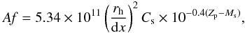 (1)where rh is the heliocentric distance in AU, dx is the detector pixel size in arcsec, Cs is the pixel signal in e−/s, and Zp and Ms are the zero points and the solar magnitude in the used filter. An example of one of the r-band-calibrated images is shown in Fig. 1.
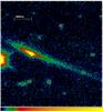 |
Fig. 1 Af calibrated SLOAN r-band image of VW139. North is up, ast is to the left. The antisolar direction is at PA = 65.2°. The image covers a region of 75 000 × 75 000 km2. This is the last image of the series acquired in r, i.e., the one with the near-by bright star at the maximum distance (visible in the E direction). The color look-up table is logarithmic, with black (left side of the color bar) corresponding to Af = 0 and yellow (right side of the bar) to Af = 1 × 10⁻⁷. |
2.2. Spectroscopy
The visible spectrum of VW139 was obtained on the same night immediately after the images. We used the R300B and R300R grisms, with dispersions of 2.48 and 3.87 Å/pixel, respectively. A 5′′ slit width was used, oriented toward the parallactic angle to minimize slit losses due to atmospheric dispersion. An image of the object in the slit is shown in Fig. 2. Three spectra with an exposure time of 300 s each were obtained with each grism, covering the 0.35–0.70 μm and 0.50–1.0 μm spectral ranges at an airmass of X = 1.1.
Images of the spectra were bias- and flat-field-corrected with lamp flats. The two-dimensional spectra were wavelength-calibrated with Xe + Ne + HgAr lamps. After the wavelength calibration, sky background was subtracted. We fitted a first-order constant sky level using a section across the spatial direction, and selecting two regions close enough to the MBC, but carefully avoiding any contribution from the observed tail. This procedure was repeated across the spectral direction every 50 pixels. After background subtraction, a one-dimensional spectrum of the optocenter of the MBC was extracted using a very narrow extraction aperture of only ± 3 pixels (the FWHM measured for the central part of the MBC is ~6 pixels) to minimize the dust contribution. To correct for telluric absorption and to obtain the relative reflectance, a G star from the Landonlt (1992) list was observed using the same spectral configuration at an airmass (X = 1.2) similar to that of the object, and was used as a solar analogue star. Each individual spectrum of the object was then divided by the corresponding spectra of the solar analog and then normalized to unity at 0.55 μm. The three individual spectra were averaged, obtaining a mean spectrum for each of the two grisms. Those spectra were finally merged using the common wavelength interval 0.60–0.70 μm. The final reflectance spectrum in the 0.38–0.9 μm region is shown in Fig. 2.
The MBC spectrum was also flux-calibrated using observations of the standard star G191 (observed the same night) and standard procedures. The flux-calibrated spectrum of VW139 was used to derive an upper limit for the CN production rate (see Sect. 3.2).
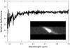 |
Fig. 2 Final reflectance spectrum of VW139. We also show an image of the asteroid inside the slit. |
3. Data analysis
3.1. Analysis of the images
In Fig. 1 the object clearly presents a narrow and almost linear tail that extends up to 40 000 km in the anti-solar direction (position angle PA ~ 63°) and more than 80 000 km in the direction of the object’s orbit plane (PA ~ 250°). This image is typical of comets when observed with the observer very close to the comet’s orbital plane and, as we show in Sect. 4, implies a dust ejection that lasted several months.
We first studied the color of the dust tail by computing the spectral slope S′ from the r-band by the g-band images using  (2)where Fr and Fg are the flux-calibrated r- and g images, and FgS and FrS are the flux of the Sun in the g and r band. The FgS/FrS ratio is computed by using the solar color (g − r)S = 0.44. The central wavelength of the g and r filters are 4844 and 6228 Å.
The color of the dust in the tail is slightly redder than the Sun, with S′ between 6% and 3%/1000 Å.
The absolute magnitude of VW139 is H = 16.1 according to the Minor Planet Center (MPC), and was computed when the asteroid was not active. We performed aperture photometry of the MBC using an aperture radius of 5′′ to determine a lower limit for the asteroid magnitude (asteroid + ejected dust in the aperture) and a lower limit for H on both filters.
We applied this only to the last two combined images of each filter (because a bright star was too close to the asteroid in the first two images). The measured magnitudes are r = 19.07 and 19.14, and g = 19.60 and 19.63, and thus the corresponding absolute magnitude lower limits are Hr = 15.16 ± 0.04 and Hg = 15.67 ± 0.02 (assuming the typical G value of 0.15 of the IAU H,G system). Of course this is a lower limit, because the dust of the tail contributes to the asteroid luminosity. The results are compatible with the value of H given by the MPC. Considering that we assumed G = 0.15, the uncertainties on the derived Hr and Hg lower limits are about 0.1−0.2 mag. Our Hr determination is compatible with the Hr = 15.1−15.0 ± 0.1 reported by Hsieh et al. (2012) between Nov. 05 and Dec. 04, 2011.
3.2. Analysis of the spectrum
The obtained reflectance spectrum of the optocenter of VW139 is very similar to that of a C-type asteroid, almost neutral in the 0.5−0.9 μm region (with a spectral slope  %/1000 Å), and a UV drop below 0.55 μm.
Because the object was active, the obtained spectrum is “contaminated” by scattered light from the dust tail. The photometry reported in the previous section and the absolute magnitude reported in the MPC show that in an aperture of 5 arcsec, the flux from the dust is about twice that reflected by the asteroid surface. Hsieh et al. (2012) reported a value of 2.5. For that reason, and considering that the PSF of the asteroid is much steeper than that of the tail, we used a very small extraction aperture of 0.8 arcsec to minimize the dust contribution. In this small aperture it is too difficult to evaluate how significant the contribution of the dust is, but in any case it is less than for a larger aperture. The difference in color between this spectrum ( ) and the color measured in the tail in the previous section (S′ = 0.5) suggests that a large part of the light in this aperture comes from the asteroid surface.
However, the color of the dust close to the asteroid is slightly redder than the Sun, as shown in the previous section. The spectra of the dust cometary coma are usually featureless and reddish in the wavelength range of the presented VW139 spectrum, but the spectrum of the asteroid itself might be bluish, as is typical of a B-type asteroid. A spectrum of VW139 when it is inactive is desiderable to accurately determine its taxonomical classification.
A bluish to almost neutral spectral slope is atypical of active comets and in cometary nuclei (Kolokolova et al. 2004; Licandro et al. 2007).
Hsieh et al. (2012) also published a spectrum of VW139 obtained a week before our observations. To compare ours with their results, both spectra are shown in Fig. 3. The spectrum of Hsieh et al. (2012), with a lower S/N, is very similar to ours below 6500 Å and slightly redder at longer wavelengths. Hsieh et al. (2012) reported a spectral slope  %/1000 Å, computed using the 0.4–0.9 μm spectral range. If, as is usually done by convention, we only consider the 0.5–0.9 μm region (to avoid the UV drop-off), the spectral slope is
  %/1000 Å, still slightly redder than ours.
The similarities between both spectra in the blue region (below 5500 Å) is a clear indication that the differences are not caused byo problems related to differential extinction (the Hsieh et al. spectrum was obtained without the orientation toward the parallactic angle) and/or by slit losses, because, in that case, the blue region of the spectrum is the most affected. One possibility is that because the Hsieh et al. spectrum was obtained with the slit aligned with the tail, maybe the aperture used to extract their spectrum was wider than the one we used (1.5′′), and consequently they might have included a larger amount of dust.
 |
Fig. 3 Comparison of the reflectance spectra of VW139 presented in this paper (blue) and that from Hsieh et al. (2012) (green). We have also included in the plot the reflectance spectrum of 133P/Elst-Pizarro (red) from Licandro et al. (2011b). The two spectra of VW139 are shifted vertically by 0.5 for clarity. |
Licandro et al. (2011) analyzed the nature of MBCs based on their spectra. In Fig. 3 our spectrum of VW139 is also compared to the spectrum of 133P/Elst-Pizarro published by Licandro et al. The spectra are very similar, therefore the conclusions about the nature of 133P in Licandro et al. (2011) can be reproduced here for VW139: the spectrum of VW139 resembles that of asteroids of the C-complex and is significantly different from those of the large majority of observed cometary nuclei, typically D- or P-types.
We also searched for any signature of gas emission that is typically observed in cometary comae, of which that of CN (B –X
–X ) at ~3800 Å is the most prominent. The detection of gas emission would be a strong test to determine if the observed tail and coma are produced by ice sublimation as in normal comets.
In Fig. 4 we show a zoom of our flux-calibrated spectrum of VW139 in the wavelength region of this CN band and compare it with the spectrum of active Jupiter family comet 8P/Tuttle (Lara, pers. comm.). None of the molecular bands, in particular the CN emission, which is clearly seen in the spectrum of 8P centered at 3870 Å, are detected in the spectrum of VW139. Hsieh et al. (2012) also failed to detect CN emission in their lower S/N spectrum obtained a week before ours.
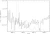 |
Fig. 4 Visible spectrum of VW139 (solid line) in the region of the CN and C3 emission bands (in erg cm-2 s-1 Å-1) compared to the spectrum of active comet 8P/Tutle (dashed line) obtained on Jan. 1, 2008 (Lara, pers. comm.). The spectrum of VW139 is averaged over an aperture of 40 pixels, i.e., 10.16 arcsec, meaning 12 300 km at the comet distance, and is multiplied by 50 for a better comparison with the spectrum of 8P/Tuttle. |
An upper limit to the CN production rate is achieved by studying the flux measure in the 3830−3905 Å range in an aperture of 40 pixels, i.e., 10.16 arcsec, meaning 12 300 km at the comet distance. We also measured the continuum that borders the band at 3770−3815 Å and 3910−3970 Å by approximating the continuum contribution by interpolating the left- and right-hand continua. Any remaining flux in the 3830−3905 Å region represents a 1σ upper limit to the CN emission.
We converted the emission band flux into column density using the g-factor from Schleicher (1957) at the asteroid heliocentric velocity of 2.124 km s-1 and distance of 2.524 AU. The resulting g-factor is g = 3.217 × 10⁻¹ erg s-1 molecule-1.
To compute the gas production rate, we assumed the Haser modeling (Haser 1957) with the CN parent velocity vp scaled with rh ( km s-1), and vd = 1 km s-1 for CN itself. The CN parent scale length is 13 000 km, whereas the CN one is 210 000 km (A’Hearn et al. 1995). With this set of parameters, the Haser modeling provides a CN 1σ production rate upper limit of 3.76 × 10²³ s-1, i.e. 3σ of 1.13 × 1024 s-1.
Our determination is on the same order of magnitude as the one reported by Hsieh et al. (2012), who obtained a value of 1.3 × 1024 s-1.
However, this does not mean that there is no gas emission and/or that a reasonable upper limit of the production rate of H2O (QH2O) can be derived from it. A limit from QH2O is usually determined assuming the average ratio QCN/QOH and QOH/QH2O of Jupiter-family comets (e.g. Hsieh et al. 2012; Licandro et al. 2011). But, as noticed by Licandro et al. (2011), this is probably meaningless, because MBCs likely formed closer to the Sun than “normal” comets. This implies a higher temperature, therefore one would expect a much lower fraction of species that are more volatile than water ice with respect to water ice, i.e., QCN/QOH is probably much lower for the MBCs than for “normal” comets.
4. The dust model
We analyzed the asteroid images by a direct Monte Carlo dust tail model, which is based on previous works on cometary dust tail analysis (e.g. Moreno 2009; Moreno et al. 2010), and on the characterization of the dust environment of comet 67P/Churyumov-Gerasimenko before Rosetta’s arrival in 2014 (the so-called Granada model, see Fulle et al. 2010).
Briefly, the code computes the trajectory of a large number of particles ejected from a cometary nucleus surface, which are exposed to solar gravity and radiation pressure. The gravity of the asteroid itself is neglected, which is a good approximation for small-sized objects.
In an ice-sublimation-driven scenario, the particles are accelerated by gas drag to their terminal velocities, which are the input velocities considered in the model. Particle ejection by any other mechanism (e.g., a collision) can also be simulated. Once ejected, the particles describe a Keplerian trajectory around the Sun, whose orbital elements are computed from the terminal velocity and the ratio of the force exerted by the solar radiation pressure and the solar gravity β (see Fulle 1989). This parameter can be expressed as β = CprQpr/(2ρr), where Cpr = 1.19 × 10⁻³ kg m-2, and ρ is the particle density, assumed to be ρ = 1000 kg m-3. For particle radii r > 0.25 μm, the radiation pressure coefficient is Qpr ~ 1 (Burns et al. 1979). To compare the model results with the observed isophotes, for CPU and memory reasons, we rebinned the original image by 2 × 2 pixels so that its spatial resolution becomes 310 km pixel-1.
For the observation date, we computed the trajectories of a large number of dust particles and calculated their positions on the (N,M) plane. M is the projected Sun-comet radius vector, and N is perpendicular to M in the opposite half-plane with respect to the nucleus velocity vector. Then, we computed their contribution to the tail brightness.
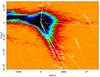 |
Fig. 5 Syndyne-synchrone diagram overimposed on a VW139 image. The density of the particles is assumed at ρ = 1000 kg m-3. The synchrones are shown as solid white lines, and correspond, in clockwise order, to +108, +81, +54, +27, 0, −27, and −54 days to perihelion, as labeled. Syndynes are shown as white dashed lines, and correspond to 0.0012, 0.0025, 0.01, and 0.05 cm, as labeled. The M- and N-axis are scaled independently to avoid label crowding. The bright feature on the left centered at approximate coordinates (− 5000,7000) corresponds to a a bright field star that can be seen in Fig. 1 placed near the middle of the left ordinate axis. |
For a first approximation of the input parameters to impose on the dust model, we first obtained a syndyne-synchrone diagram. Figure 5 shows this map with seven synchrones from +108 to −54 days to perihelion, and three syndynes corresponding to particle radii of 12, 25, and 100 μm. The M- and N-axis are scaled independently to avoid label crowding. Based on this map, and since the observation was made about 130 days post-perihelion, we infer that the onset of the asteroid activity should have occurred around perihelion, lasting close to the observation date, as a first approximation.
The synthetic tail brightness depends on the ejection velocity law assumed, the particle size distribution, the dust mass loss rate, as well as on the geometric albedo of the particles. We assumed isotropic ejection. To constrain the number of free parameters, the size distribution was assumed to be independent of time and to be characterized by a power-law with index α. The maximum size of the ejected particles is set by the escape velocity. If H = 16.1, and the albedo is pv ~ 0.05, the asteroid radius would be R ~ 1.8 km. If the bulk density is ρ = 1000 kg m-3, the escape velocity would be about 0.3 m s-1, assuming a spherical object. Based on the syndyne-synchrone locus, we set the lower limit of particle sizes at 1 μm. Smaller particles ejected some 30 days before the observation would be beyond the image limits.
Then, we ran the code for a large number of input dust loss masses and particle velocities as functions of the heliocentric distance. The velocity was assumed to vary with β as v ∝ β1/2. The best fit is shown in Fig. 6, whereas the dust loss rates and particle velocities are shown in Fig. 7. Our best-fit model used a power-law size distribution function with power index of −3.1, which is in the range of the estimates for other comets and MBCs. For the escape velocity, we found vesc = 0.2 m s-1 as the best-fit. With this value for the escape velocity, we derived from the model that the largest ejected particles forming the anti-sunward branch are about 200 μm in radius. If the escape velocity is assumed to be higher than 0.2 m s-1, the maximum size of those particles would be smaller, and the model would be unable to fit that anti-sunward branch. This is clear from the syndyne-synchrone network of Fig. 6, which indicates that this feature can be fitted by particles of size ~100 μm or larger. On the other hand, if vesc were slower than ~0.2 m s-1, it would be possible to fit the dust feature, because particles in excess of 200 μm could be ejected.
The total dust mass ejected derived from the model is ~2 × 10⁶ kg, about 2 × 10⁻⁵% of the total mass of the asteroid. The activity onset is shortly after perihelion, and lasts about 100 days (see Fig. 7). This mass loss peaks some 60 days after perihelion at 0.5 kg s-1, and is correlated with the ejection velocity. This is compatible with the early observations of Hsieh et al. (2011), which describe the object as having a non-stellar PSF on August 30, about 45 days after perihelion. On the other hand, the velocities are consistent with expectations of cometary activity at 2.5 AU from the Sun, which supports the assumption that water ice sublimation is the mechanism that ejected the observed dust.
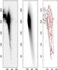 |
Fig. 6 Left: median-averaged image of VW139 obtained on November 29, 2011, referred to the (N,M) plane. Center: modeled image. Right: comparison of observed isophotes (black) and modeled isophotes (red). The contour levels are 5 × 10-15, 10-14, and 2 × 10-14, in solar disk intensity units. Each pixel corresponds to 310 km. |
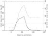 |
Fig. 7 Derived mass loss rate (solid line, left vertical axis) and ejection velocity (dashed line, right vertical axis), as a function of time. The ejection velocity refers to a 0.01 cm particle. The dotted line indicates the assumed escape velocity. |
5. Discussion and conclusions
The principal aim of studying MBCs is, as explained in the introduction, to understand their activation mechanism and origin. Are they comets, or asteroids that, under certain circumstances, eject dust?
Images of the ejected dust can help us to understand what the dust ejection mechanism is. The images of 2006 VW139 obtained on November 29, 2011 with the OSIRIS camera-spectrograph at the 10.4 m GTC (El Roque de los Muchachos Observatory, La Palma, Canary Islands, Spain) show an object that presents a narrow, almost linear tail that extends up to 40 000 km in the anti-solar direction and more than 80 000 km in the direction of the object’s orbit plane. This tail is typical of comets observed very close to the comet’s orbital plane. Moreover, the color map shows that the tail in the anti-solar direction is significantly redder, which indicates that the larger particles concentrate in this region, as expected for an object that presents a comet-like activity.
Using a direct Monte Carlo dust tail model (e.g. Moreno 2009; Moreno et al. 2010), we fitted the images and derived the mass loss rates and ejection velocity as a function of time. We first concluded that the observed tail is not compatible with a short-lasting event like a collision or an outburst. The activity onset occurs shortly after perihelion, and lasts about 100 days. All evidence favors a comet-like ejection mechanism, which means dust ejected by the sublimation of volatiles.
We were also able to derive other properties of the ejected dust and the object itself. From the dust model, and to fit the sunward branch intensities, the best-fit escape velocity derived was vesc = 0.2 m s-1.
On the other hand, the mass loss peaks some 60 days after perihelion at 0.5 kg s-1, and is correlated with the ejection velocity. This is compatible with the early observations of Hsieh et al. (2011), which describe the object as having a non-stellar PSF (indicative of a dust cloud around the object), on August 30 (45 days after perihelion). The derived velocities are also consistent with expectations of cometary activity at 2.5 AU from the Sun. The total mass ejected is ~2 × 10⁶ kg.
The spectrum of the object can be compared with spectra of comets and primitive asteroids to determine which group the object belongs to, and to search for gas species in the coma (which would confirm of a comet-like activation mechanism). The reflectance spectrum of the optocenter of VW139 is typical of a C-type asteroid, almost neutral in the 0.5–0.9 μm region (with a spectral slope %/1000 Å), and a UV drop below 0.55 μm. A bluish to almost neutral slope in the spectrum is atypical of active comets but typical of MBCs (Licandro et al. 2011). Accordingly, VW139 presents a spectrum typical of the asteroids with similar semi-major axis and different from those of comet nuclei. This supports an in situ origin, as for dynamical simulations.
We finally searched for the CN (B ) signature of gas emission at ~3800 Å that is typically observed in cometary comae, finding no evidence of this feature in our spectrum. We derived an upper limit of the CN production rate QCN = 3.76 × 10²³ s-1. Unfortunately, the direct determination of QH2O is very difficult, and to derive an upper limit of QH2O based on the upper limit of QCN, we had to assume values of the QCN/QOH and QOH/QH2O ratios that are typical of comets. This last assumption might not be correct for MBCs, as explained in Sect. 3.2.
In conclusion, (300163) 2006 VW139, like other well-studied MBCs (see the case of 133P/Elst-Pizarro) is likely a primitive C-type asteroid that has a water-ice reservoir at subsurface depth. Owing to still uncertain mechanisms (probably a collision that eroded its surface), this reservoir has recently been exposed to sunlight or to temperatures that produce enough heat to sublime the ice and drag dust from the surface.
Acknowledgments
We thank H. Hsieh for providing the ascii version of their spectrum and to the anonymous referee who helped to improve this paper. J.L. acknowledges support from the project AYA2011-29489-C03-02 (MEC). L.M.L.’s and J.d.L.’s work has been funded through project AYA 2009-08011 awarded by the Spanish “Ministerio de Ciencia e Innovación”. J.d.L. aslo acknowledges financial support from the current Spanish “Secretaría de Estado de Investigación, Desarrollo e Innovación” (Juan de la Cierva contract). F.M. was supported by contracts AYA2009-08190 and FQM-4555 (Junta de Andalucía). Based on observations made with the Gran Telescopio Canarias (GTC), installed in the Spanish Observatorio del Roque de los Muchachos of the Instituto de Astrofísica de Canarias, on the island of La Palma.
References
- A’Hearn, M. C., Millis, R. L., Schleicher, D. G., Osip, D. J., & Birch, P. V. 1995, Icarus, 118, 223 [NASA ADS] [CrossRef] [Google Scholar]
- Bagnulo, S., Tozzi, G. P., Boehnhardt, H., Vincent, J.-B., & Muinonen, K. 2010, A&A, 514, A99 [NASA ADS] [CrossRef] [EDP Sciences] [Google Scholar]
- Boehnhardt, H., Sekanina, Z., Fiedler, A., et al. 1997, Highlights Astron., 11, 233 [Google Scholar]
- Burns, J. A., Lamy, P. L., & Soter, S. 1979, Icarus, 40, 1 [NASA ADS] [CrossRef] [Google Scholar]
- Campins, H., Hargrove, K., Pinilla-Alonso, N., et al. 2010, Nature, 464, 1320 [NASA ADS] [CrossRef] [PubMed] [Google Scholar]
- Cepa, J. 2010, Highlights of Spanish Astrophysics V, ApS&S Proc. (Springer-Verlag), 15 [Google Scholar]
- Cepa, J., Aguiar, M., Escalera, V. G., et al. 2000, Proc. SPIE, 4008, 623 [Google Scholar]
- Elst, E., Pizarro, O., Pollas, C., et al. 1996, IAUC 6456 [Google Scholar]
- Fernández, J., Gallardo, T., & Brunini, A. 2002, Icarus, 159, 358 [NASA ADS] [CrossRef] [Google Scholar]
- Fulle, M. 1989, A&A, 217, 283 [NASA ADS] [Google Scholar]
- Fulle, M., Colangeli, L., Agarwal, J., et al. 2010, A&A, 525, A63 [NASA ADS] [CrossRef] [EDP Sciences] [Google Scholar]
- Haser, L. 1957, Bull. Soc. Roy. Sci. Liege, 43, 740 [Google Scholar]
- Hsieh, H., & Jewitt, D. 2006, Science, 312, 561 [NASA ADS] [CrossRef] [PubMed] [Google Scholar]
- Hsieh, H., Jewitt, D., & Fernández, Y. 2004, AJ, 127, 299 [Google Scholar]
- Hsieh, H., Jewitt, D., & Fernández, Y. 2009, ApJ, 694, 111 [Google Scholar]
- Hsieh, H., Jewitt, D., Lacerda, P., Lowry, S., & Snodgrass, C. 2010, MNRAS, 403, 363 [NASA ADS] [CrossRef] [Google Scholar]
- Hsieh, H., et al. 2011, IAUC 2920 [Google Scholar]
- Hsieh, H., Yang, B., Haghighipour, N., et al. 2012, ApJ, 748, L15 [NASA ADS] [CrossRef] [Google Scholar]
- Kolokolova, L., Hanner, M. S., Levasseur-Regourd, A.-C., & Gustafson, B. 2004, in Comets II, eds. M. C. Festou, H. U. Keller, & H. A. Weaver (Tucson, AZ: Univ. Arizona Press), 577 [Google Scholar]
- Landolt, A. U. 1992, AJ, 104, 340 [NASA ADS] [CrossRef] [Google Scholar]
- Levison, H., Bottke, W., Gounelle, M., et al. 2009, Nature, 460, 364 [NASA ADS] [CrossRef] [PubMed] [Google Scholar]
- Licandro, J., Campins, H., Mothé-Diniz, T., Pinilla-Alonso, N., & de León, J. 2007, A&A, 461, 751 [NASA ADS] [CrossRef] [EDP Sciences] [Google Scholar]
- Licandro, J., Campins, H., Kelley, M., et al. 2011a, A&A, 525, A34 [NASA ADS] [CrossRef] [EDP Sciences] [Google Scholar]
- Licandro, J., Campins, H., Tozzi, G. P., et al. 2011b, A&A, 532, A65 [NASA ADS] [CrossRef] [EDP Sciences] [Google Scholar]
- Moreno, F. 2009, ApJS, 183, 33 [NASA ADS] [CrossRef] [Google Scholar]
- Moreno, F., Licandro, J., Tozzi, G. P., et al. 2010, ApJ, 718, 132 [NASA ADS] [CrossRef] [Google Scholar]
- Moreno, F., Licandro, J., Ortiz, J. L., et al. 2011a, ApJ, 738, 130 [NASA ADS] [CrossRef] [Google Scholar]
- Moreno, F., Lara, L., Licandro, J., et al. 2011b, ApJ, 738, 16 [Google Scholar]
- Novakovic, B., Hsieh, H. H., & Cellino, A. 2012, 424, 1432 [Google Scholar]
- Rivkin, A. S., & Emery, J. 2010, Nature, 464, 1322 [NASA ADS] [CrossRef] [PubMed] [Google Scholar]
- Schorghofer, N. 2008, ApJ, 682, 697 [NASA ADS] [CrossRef] [Google Scholar]
- Schleicher, D. G. 2010, AJ, 140, 973 [NASA ADS] [CrossRef] [Google Scholar]
- Tozzi, G. P., Boehnhardt, H., Kolokolova, L., et al. 2007, A&A, 476, 979 [NASA ADS] [CrossRef] [EDP Sciences] [Google Scholar]
- Toth, I. 2006, A&A, 446, 333 [NASA ADS] [CrossRef] [EDP Sciences] [Google Scholar]
All Tables
All Figures
|
Fig. 1 Af calibrated SLOAN r-band image of VW139. North is up, ast is to the left. The antisolar direction is at PA = 65.2°. The image covers a region of 75 000 × 75 000 km2. This is the last image of the series acquired in r, i.e., the one with the near-by bright star at the maximum distance (visible in the E direction). The color look-up table is logarithmic, with black (left side of the color bar) corresponding to Af = 0 and yellow (right side of the bar) to Af = 1 × 10⁻⁷. |
| In the text | |
|
Fig. 2 Final reflectance spectrum of VW139. We also show an image of the asteroid inside the slit. |
| In the text | |
|
Fig. 3 Comparison of the reflectance spectra of VW139 presented in this paper (blue) and that from Hsieh et al. (2012) (green). We have also included in the plot the reflectance spectrum of 133P/Elst-Pizarro (red) from Licandro et al. (2011b). The two spectra of VW139 are shifted vertically by 0.5 for clarity. |
| In the text | |
|
Fig. 4 Visible spectrum of VW139 (solid line) in the region of the CN and C3 emission bands (in erg cm-2 s-1 Å-1) compared to the spectrum of active comet 8P/Tutle (dashed line) obtained on Jan. 1, 2008 (Lara, pers. comm.). The spectrum of VW139 is averaged over an aperture of 40 pixels, i.e., 10.16 arcsec, meaning 12 300 km at the comet distance, and is multiplied by 50 for a better comparison with the spectrum of 8P/Tuttle. |
| In the text | |
|
Fig. 5 Syndyne-synchrone diagram overimposed on a VW139 image. The density of the particles is assumed at ρ = 1000 kg m-3. The synchrones are shown as solid white lines, and correspond, in clockwise order, to +108, +81, +54, +27, 0, −27, and −54 days to perihelion, as labeled. Syndynes are shown as white dashed lines, and correspond to 0.0012, 0.0025, 0.01, and 0.05 cm, as labeled. The M- and N-axis are scaled independently to avoid label crowding. The bright feature on the left centered at approximate coordinates (− 5000,7000) corresponds to a a bright field star that can be seen in Fig. 1 placed near the middle of the left ordinate axis. |
| In the text | |
|
Fig. 6 Left: median-averaged image of VW139 obtained on November 29, 2011, referred to the (N,M) plane. Center: modeled image. Right: comparison of observed isophotes (black) and modeled isophotes (red). The contour levels are 5 × 10-15, 10-14, and 2 × 10-14, in solar disk intensity units. Each pixel corresponds to 310 km. |
| In the text | |
|
Fig. 7 Derived mass loss rate (solid line, left vertical axis) and ejection velocity (dashed line, right vertical axis), as a function of time. The ejection velocity refers to a 0.01 cm particle. The dotted line indicates the assumed escape velocity. |
| In the text | |
Current usage metrics show cumulative count of Article Views (full-text article views including HTML views, PDF and ePub downloads, according to the available data) and Abstracts Views on Vision4Press platform.
Data correspond to usage on the plateform after 2015. The current usage metrics is available 48-96 hours after online publication and is updated daily on week days.
Initial download of the metrics may take a while.