| Issue |
A&A
Volume 549, January 2013
|
|
|---|---|---|
| Article Number | A111 | |
| Number of page(s) | 5 | |
| Section | Astronomical instrumentation | |
| DOI | https://doi.org/10.1051/0004-6361/201220586 | |
| Published online | 08 January 2013 | |
Efficient Wiener filtering without preconditioning
1
Institut d’Astrophysique de Paris, UMR 7095, CNRS, Université Paris 6 –
Pierre et Marie Curie
98bis Bd Arago,
75014
Paris,
France
e-mail: elsner@iap.fr
2
Departments of Physics and Astronomy, University of Illinois at
Urbana-Champaign, Urbana, IL
61801,
USA
Received: 18 October 2012
Accepted: 20 November 2012
We present a new approach to calculate the Wiener filter solution of general data sets. It is trivial to implement, flexible, numerically absolutely stable, and guaranteed to converge. Most importantly, it does not require an ingenious choice of preconditioner to work well. The method is capable of taking into account inhomogeneous noise distributions and arbitrary mask geometries. It iteratively builds up the signal reconstruction by means of a messenger field, introduced to mediate between the different preferred bases in which signal and noise properties can be specified most conveniently. Using cosmic microwave background (CMB) radiation data as a showcase, we demonstrate the capabilities of our scheme by computing Wiener filtered WMAP7 temperature and polarization maps at full resolution for the first time. We show how the algorithm can be modified to synthesize fluctuation maps, which, combined with the Wiener filter solution, result in unbiased constrained signal realizations, consistent with the observations. The algorithm performs well even on simulated CMB maps with Planck resolution and dynamic range.
Key words: methods: data analysis / methods: statistical / cosmic background radiation
© ESO, 2013
1. Introduction
Signal reconstruction out of noisy data is arguably one of the most fundamental problems in astronomy (and science in general), and has been subject of extensive research for centuries. The method of least squares, for example, was originally introduced to predict the orbital parameters of the dwarf planet 1 Ceres out of a series of astrometric measurements (Gauss 1809). Since then, applications in signal processing have become legion.
Incorporating statistical information about the properties of noise and signal laid the foundation for a large class of powerful reconstruction techniques, including particularly popular methods such as the Wiener filter (Wiener 1949), approaches that rely on entropy maximization (Jaynes 1957), or the Kalman filter (Kálmán 1960). The issue has remained a topic of ongoing research. For Gaussian fields, only recently efficient algorithms have been developed for cases without prior knowledge of the signal properties (e.g., Wandelt et al. 2004; Jasche et al. 2010; Enßlin & Frommert 2011), or, where neither signal nor noise covariances are known a priori (Oppermann et al. 2011).
In this paper, we focus on the evaluation of the generalized Wiener filter. If the observed data d are a linear combination of signal s and noise n,  (1)the Wiener filter is defined as the solution of the equation
  (2)Then, by construction, sWF is the maximum a posteriori probability solution if signal and noise are both Gaussian random fields with known covariances S and N, respectively.
The Wiener filter or variants thereof are frequently encountered in the post-processing of observational data. In the analysis of cosmic microwave background (CMB) radiation experiments, for example, during optimal power spectrum estimation (e.g., Tegmark 1997b; Bond et al. 1998; Oh et al. 1999; Elsner & Wandelt 2012a), likelihood analysis (e.g., Hinshaw et al. 2007; Dunkley et al. 2009; Elsner & Wandelt 2012b), mapmaking (e.g., Tegmark et al. 1997; Tegmark 1997a), and lensing reconstructions (e.g., Hirata et al. 2004; Smith et al. 2007), etc.
In practice, the numerical computation of Eq. (2) can be challenging for the large data sets collected by modern experiments. The underlying difficulty is that signal and noise covariances grow as the square of the size of the data set and become too large to be stored and processed as dense matrices. Progress is possible when these matrices are structured, e.g. when there are sets of bases where S and N become sparse. However, the bases may be incompatible, for example, the signal covariance may be sparse in Fourier space, whereas the noise covariance may be sparse in pixel space. As a result, one can either solve the Wiener filter equation only approximately, e.g. by assuming a homogeneous and isotropic noise distribution (as done in, e.g., Hirata et al. 2004; Komatsu et al. 2005; Mangilli & Verde 2009), or has to rely on complex and costly numerical schemes (e.g., involving conjugate gradient solvers with multigrid preconditioners, Smith et al. 2007). Finding fast preconditioners that work is a highly non-trivial art especially since the matrices of interest are often extremely ill-conditioned, with typical condition numbers of the order  .
.
The Wiener filter is the optimal linear filter only for strictly Gaussian noise and signal. However, a maximum entropy argument shows that the Gaussian prior is the least informative prior, once mean and covariance of the random fields are specified. From a Bayesian point of view, a Gaussian prior can therefore be a well-justified approximation even for non-Gaussian inference. This argument provides a theoretical underpinning for the work of, e.g, Bouchet et al. (1999), where the authors use Wiener filtering as a means to clean CMB maps from (non-Gaussian) foregrounds. Applied in the limit of weak non-Gaussianity, the Wiener filter has also proven an indispensable tool for the search for primordial non-Gaussianity in CMB data (Komatsu et al. 2005), where inference from the full non-Gaussian posterior is computationally very demanding (Elsner & Wandelt 2010).
In this paper, we propose a high precision, iterative algorithm for the solution of the exact Wiener filter equation. It is conceptually very simple and therefore easy to implement correctly, yet still numerically efficient enough to be of general interest. The method is fully universal as long as there exist easily accessible orthogonal basis sets which render S and N sparse. We illustrate our approach by applying it to CMB signal reconstruction.
The paper is organized as follows. In Sect. 2, we introduce our new algorithm for the efficient calculation of the Wiener filter. We then present an explicit example and analyze CMB data of the WMAP experiment (Sect. 3) showing how to generalize Eq. (1) to include an instrumental transfer function. Finally, we summarize our findings in Sect. 4. Throughout the paper, we assume WMAP7+BAO+H0 cosmological parameters (Komatsu et al. 2011).
2. Method
In the following, we present the basic equations of the algorithm and address how to solve them numerically before discussing a concrete example.
2.1. Algorithm for Wiener filtering
For an efficient evaluation of Eq. (2), we introduce an additional stochastic auxiliary field t with covariance T. The statistical properties of this helper variable are deliberately chosen very simple: T is proportional to the identity matrix. The identity matrix is invariant under any orthogonal basis change. While it may not be possible to directly apply expressions like (S + N)-1 to a data vector, we can always do so with combinations as (S + T)-1 and (N + T)-1 regardless of which basis renders S or N sparse.
In order to take advantage of this possibility, we form a set of equations to be solved iteratively for the signal reconstruction s and the auxiliary field t, ![\begin{eqnarray} \label{eq:def_algorithm1} \left( \Nbar^{-1} + (\lambda \T)^{-1} \right) \, t && = \Nbar^{-1} \, d + (\lambda \T)^{-1} \, s \\[2mm] \label{eq:def_algorithm2} \left( \S^{-1} + (\lambda \T)^{-1} \right) \, s && = (\lambda \T)^{-1} \, t \, , \end{eqnarray}](/articles/aa/full_html/2013/01/aa20586-12/aa20586-12-eq15.png) where we defined
where we defined  and introduced one additional scalar parameter λ, whose usefulness we will discuss in the context of convergence acceleration in Sect. 2.2. We choose the amplitude of the covariance matrix of the auxiliary field according to T = τ1 with τ ≡ min(diag(N)). Consequently, the field t gains a physical interpretation: it corresponds to a signal reconstruction given the fraction of the noise that is distributed homogeneously and isotropically in the data. It can be easily shown that the above system reduces to the Wiener filter equation in the limit λ = 1.
The algorithm can be summarized as follows. We initialize the vectors s and t with zeros. First, we solve Eq. (3) for the auxiliary field t in the basis defined by the noise covariance matrix. Next, we change the basis to, e.g., Fourier space, where S can be represented easily. Then, we solve for s using Eq. (4) given the latest realization of t, and finally transform the result back to the original basis. After a sufficient number of iterations, the signal reconstruction converges to the Wiener filter solution, s → sWF as we show now.
2.2. Stability, convergence speed and diagnostics
The method is unconditionally stable. If the residual is ϵi at one iteration, it will be ![\begin{equation} \label{eq:epsilon} \epsilon_{i+1}=\left[ \S (\S + \lambda \T)^{-1} \right] \left[ \Nbar (\Nbar + \lambda \T)^{-1} \right] \epsilon_{i} \end{equation}](/articles/aa/full_html/2013/01/aa20586-12/aa20586-12-eq23.png) (5)at the next. If N ∝ 1, the system is solved in a single iteration. The terms in square brackets have spectral radii ρ1, 2 strictly less than unity. So |ϵi + 1| < ρ1ρ2 |ϵi| for all i, and convergence is exponential. It is fast for low noise pixels and signal modes with low prior variance, and slowest for modes with high prior variance in high noise pixels. Temporarily setting λ > 1 accelerates convergence in this problematic regime.
(5)at the next. If N ∝ 1, the system is solved in a single iteration. The terms in square brackets have spectral radii ρ1, 2 strictly less than unity. So |ϵi + 1| < ρ1ρ2 |ϵi| for all i, and convergence is exponential. It is fast for low noise pixels and signal modes with low prior variance, and slowest for modes with high prior variance in high noise pixels. Temporarily setting λ > 1 accelerates convergence in this problematic regime.
For a given λ, the iterations minimize ![\begin{equation} \chi^2(x,\lambda) = x^{\dagger} \S^{-1} x + (d - x)^{\dagger} \left[ \N + (\lambda - 1) \T \right]^{-1} (d - x) \end{equation}](/articles/aa/full_html/2013/01/aa20586-12/aa20586-12-eq29.png) (6)to give s(λ) = S(S + N + (λ − 1)T)-1. Fortunately, it is precisely in the regime where convergence is slowest (S, N large) that s(λ > 1) approximates s(1) best.
(6)to give s(λ) = S(S + N + (λ − 1)T)-1. Fortunately, it is precisely in the regime where convergence is slowest (S, N large) that s(λ > 1) approximates s(1) best.
The goal is therefore to find a “cooling schedule” which starts at high λ and reduces it to λ = 1 such that the final solution satisfies a defined accuracy criterion. Note that further iterations at lower λ never degrade but always improve parts of the solution that were found at higher λ.
At x = s(λ), we have  for λ > 1. We now show that we can find a “cooling schedule” for λ which respects the error bound
  throughout.
The following algorithm has the desired property: initialize x = 0 and choose the initial λ such that χ2(λ,0) = d†(N + (λ − 1)T)-1d = b. Then iterate x once at that λ, which reduces E to χ2(λ,x). Decrease λ such that E = b. Repeat until λ = 1 at which point x = s(1).
So far we have not specified how to calculate the optimal  , which only becomes easy to compute after the Wiener Filter has been found. Choosing
  leads to a needlessly inaccurate map, containing numerical noise artifacts that could result in erroneous statistical conclusions; choosing
  , gives results that are not wrong, just suboptimal.
Fortunately, it is possible to approximate b during the solution, as long as the initial . After converging at λ > 1 when , we can increase b to make it sufficiently close to  in one step with minimal additional computation. At that point, we have x = s(λ) and can calculate
  , with the inequality being quadratically small.
If d is consistent with the assumed statistical model, d = s + n, we can find how close b should be to  . For an ensemble of data sets, is χ2-distributed with a mean given by the number of degrees of freedom, nd.o.f., and a variance of
  . Hence, no outcome of statistical inference based on the resulting Wiener Filter depends on whether it has an excess χ2(1) of much less than σχ2.
Even if we had chosen b far below the expectation, b = nd.o.f − mσχ2, with m ≳ 5, excluding a violation of for all practical purposes, the updated b′ satisifies  . It is therefore statistically irrelevant as long as nd.o.f. ≫ 1 which is true for all cases where an iterative scheme is likely to be useful.
This algorithm guarantees satisfying a given error bound, but it does not guarantee the fastest possible time to solution. For applications to the CMB, where the signal power spectrum tends to decrease with increasing scale, it is much cheaper to iterate at high λ than at low λ. In Sect. 3, we describe a heuristic choice for the “cooling schedule” that exploits the assumed shape of the signal power spectrum and leads to significantly faster execution times.
2.3. Constrained realizations
The Wiener filter is known to remove noise very aggressively. As a result, the covariance of the signal reconstruction is reduced compared to the true signal,  (7)To obtain signal realizations with correct covariance properties that are consistent with the observed data, we have to add a fluctuation vector f to the Wiener filter solution with covariance (Bertschinger 1987, see also, e.g., Hoffman & Ribak 1991)
  (8)Applying only minor modifications, the algorithm as introduced above can be adapted to generate suitable fluctuation maps. The only difference lies in the source term on the right-hand side of Eq. (3), which we replace by
 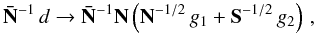 (9)where g1,2 are independent univariate Gaussian random variables. For those entries of the vector S − 1/2 g2 that fall within masked regions where
  is zero and formally no inverse N can be defined, the corresponding blocks of the matrix product
  have to be replaced with the identity matrix.
After the algorithm has been evaluated as explained in Sect. 2.1, the solution is a random realization of a fluctuation map f with the correct covariance properties. Constrained realizations are then given by sCR = sWF + f.
3. WMAP polarization analysis
We now discuss the application of our technique to Wilkinson microwave anisotropy probe (WMAP) data (Jarosik et al. 2011). We used the seven-year observations of the CMB radiation in the V-band at 61 GHz as a basis for the reconstruction1, at resolution parameter nside = 512 in the Healpix representation (Górski et al. 2005) and ℓmax = 1024. Since CMB anisotropies are isotropic and Gaussian, the signal covariance is diagonal in spherical harmonic space. The noise covariance, on the other hand, can be approximated by a diagonal matrix in pixel space (Hinshaw et al. 2003).
However, as we are interested in the Wiener filtering of temperature and polarization data, S and N are in fact block diagonal, with a significantly increased condition number of the matrices (Larson et al. 2007). For all multipole moments ℓ, we write, ![\begin{equation} S_{\ell} = b_{\ell}^2 \begin{pmatrix} C^\mathrm{TT}_{\ell} & C^\mathrm{TE}_{\ell}\\[1.5mm] C^\mathrm{TE}_{\ell} & C^\mathrm{EE}_{\ell} \end{pmatrix} \, , \end{equation}](/articles/aa/full_html/2013/01/aa20586-12/aa20586-12-eq75.png) (10)where the
(10)where the  are the power spectra for temperature (XX = TT), polarization (XX = EE), and their cross-spectrum (XX = TE), and the bℓ are the beam function. As we did not aim at a reconstruction of a possible contribution from a curl component to the polarization signal (XX = BB), we excluded it from the analysis. The blocks of the noise covariance matrix are, for every pixel,
 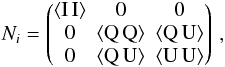 (11)where we used the Stokes parameters I, Q, and U. For WMAP data, the cross-correlations ⟨ I Q ⟩ and ⟨ I U ⟩ are small (Page et al. 2007).
We adopted the official WMAP extended temperature and polarization masks, restricting the sky fraction available to 70.6% and 73.3%, respectively. We removed possible residual monopole and dipole contributions after the masks had been applied. Avoiding numerical errors associated with spherical harmonic transforms on the cut sky can be done by an explicit low rank update of the inverse noise covariance matrix  in Eq. (3) to assign infinite variance to a set of template maps, representing the (non-cosmological) modes to be subtracted (Smith et al. 2009). However, we found it numerically more stable to split the calculation into separate steps; we therefore multiplied the input independently by
  (12)where V is a 4 × npix matrix, storing the four masked templates to be marginalized over. We used the Woodbury matrix identity to evaluate the equation.
To initialize the algorithm, we chose λ according to the ratio  at ℓiter = 20. This starting point is well suited to let all large-scale modes from ℓ ≈ 30 down to the quadrupole converge. After the χ2 has reached a plateau, we decreased it to the ratio at
  . We restricted the maximal increment in ℓiter to 500 and assured that λ ≥ 1 is always fulfilled. We achieved robust results after terminating the algorithm once Δχ2 < 10-4 σχ2 at λ = 1 has been reached, in this case at a final χ2/nd.o.f. = 0.996. The success of the algorithm does not sensitively depend on the scheme for lowering λ to unity.
The gradual decrease of λ, coupled to a well specified multipole moment ℓiter, allows for a significant speedup of the algorithm. Since the signal is build-up from large to small scales, fluctuations at multipoles ℓ > ℓiter will be suppressed. As a consequence, we can restrict the maximum multipole moment of the computationally expensive spherical harmonic transforms to  , considerably smaller than ℓmax for most of the iterations. Owing to a time complexity of
  , the overall computing time for the spherical harmonic transforms can be substantially reduced. For the final iterations including the full range of ℓ, the algorithm is an excellent candidate for further acceleration by means of the massive parallelism offered by modern graphics processing units (Elsner & Wandelt 2011).
The result of the WMAP analysis is shown in Figs. 1 and 2, where we plot patches of the Wiener filtered maps for the Stokes parameters I, Q, and U, as well as an example of a temperature fluctuation map. The non-vanishing cross-spectrum  allows for an efficient polarization reconstruction in masked regions, as long as temperature data are available. A distinguishing feature of Wiener filtering is the extrapolation of signal into the mask; this works especially well in the small areas where single point sources have been cut out.
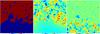 |
Fig. 1 Temperature reconstruction. Using the WMAP mask (left panel) for the analysis, we plot the V-band temperature map after Wiener filtering (middle panel). It can be supplemented to a constrained realization by superposing a fluctuation term (right panel). The patches are 25° on the side, centered at galactic coordinates (l, b) = (0°, 35°). |
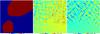 |
Fig. 2 Polarization reconstruction. Using the WMAP polarization mask (left panel) for the analysis, we obtain Wiener filtered maps for the Stokes parameters Q (middle panel), and U (right panel). The patches are 25° on the side, centered at galactic coordinates (l, b) = (0°, 35°). |
4. Discussion and conclusions
We presented an efficient technique to calculate the Wiener filter solution of general data sets. Introducing a stochastic auxiliary field with a simple covariance matrix proportional to the identity matrix, we indicated how an iterative solver for the Wiener filter equation can be constructed. The resulting algorithm is not only numerically robust, but also flexible. Using CMB temperature and polarization data obtained by the WMAP mission as an example, we explicitly demonstrated the usefulness of the method.
We estimated the numerical efficiency of the algorithm for typical CMB temperature maps as obtained with the high frequency instrument aboard the Planck satellite (Planck Collaboration 2011). At Healpix resolution nside = 2048 and ℓmax = 3000, calculating the Wiener filter solution takes about 22 CPUhrs on a single computing node comprising two quad-core Intel Xeon 2.7 GHz processors. We conclude, that the method described here is not only applicable to a wide range of problems, but also effective enough to be of general interest. We are currently exploring several further variants of the general messenger approach as well as generalizations of this method to the case of multiple data sets measuring the same underlying signal with different transfer functions or more general noise covariance matrices.
Available at http://lambda.gsfc.nasa.gov
Acknowledgments
We thank the anonymous referee for comments which helped to improve the presentation of our results. We are grateful to S. Prunet for comments on the draft of this paper. B.D.W. was supported by the ANR Chaire d’Excellence and NSF grants AST 07-08849 and AST 09-08902 during this work. F.E. gratefully acknowledges funding by the CNRS. Some of the results in this paper have been derived using the HEALPix (Górski et al. 2005) package.
References
- Bertschinger, E. 1987, ApJ, 323, L103 [NASA ADS] [CrossRef] [Google Scholar]
- Bond, J. R., Jaffe, A. H., & Knox, L. 1998, Phys. Rev. D, 57, 2117 [NASA ADS] [CrossRef] [Google Scholar]
- Bouchet, F. R., Prunet, S., & Sethi, S. K. 1999, MNRAS, 302, 663 [NASA ADS] [CrossRef] [Google Scholar]
- Dunkley, J., Komatsu, E., Nolta, M. R., et al. 2009, ApJS, 180, 306 [NASA ADS] [CrossRef] [Google Scholar]
- Elsner, F., & Wandelt, B. D. 2010, ApJ, 724, 1262 [NASA ADS] [CrossRef] [Google Scholar]
- Elsner, F., & Wandelt, B. D. 2011, A&A, 532, A35 [NASA ADS] [CrossRef] [EDP Sciences] [Google Scholar]
- Elsner, F., & Wandelt, B. D. 2012a, A&A, 540, L6 [NASA ADS] [CrossRef] [EDP Sciences] [Google Scholar]
- Elsner, F., & Wandelt, B. D. 2012b, A&A, 542, A60 [NASA ADS] [CrossRef] [EDP Sciences] [Google Scholar]
- Enßlin, T. A., & Frommert, M. 2011, Phys. Rev. D, 83, 105014 [NASA ADS] [CrossRef] [Google Scholar]
- Gauss, C. F. 1809, Theoria motus corporum coelestium in sectionibus conicis solem ambientium (Hamburgi: Sumptibus F. Perthes et I. H. Besser) [Google Scholar]
- Górski, K. M., Hivon, E., Banday, A. J., et al. 2005, ApJ, 622, 759 [NASA ADS] [CrossRef] [Google Scholar]
- Hinshaw, G., Barnes, C., Bennett, C. L., et al. 2003, ApJS, 148, 63 [NASA ADS] [CrossRef] [Google Scholar]
- Hinshaw, G., Nolta, M. R., Bennett, C. L., et al. 2007, ApJS, 170, 288 [NASA ADS] [CrossRef] [Google Scholar]
- Hirata, C. M., Padmanabhan, N., Seljak, U., Schlegel, D., & Brinkmann, J. 2004, Phys. Rev. D, 70, 103501 [NASA ADS] [CrossRef] [Google Scholar]
- Hoffman, Y., & Ribak, E. 1991, ApJ, 380, L5 [NASA ADS] [CrossRef] [Google Scholar]
- Jarosik, N., Bennett, C. L., Dunkley, J., et al. 2011, ApJS, 192, 14 [NASA ADS] [CrossRef] [Google Scholar]
- Jasche, J., Kitaura, F. S., Wandelt, B. D., & Enßlin, T. A. 2010, MNRAS, 406, 60 [NASA ADS] [CrossRef] [Google Scholar]
- Jaynes, E. T. 1957, Phys. Rev., 106, 620 [Google Scholar]
- Kálmán, R. E. 1960, Trans. ASME–J. Basic Eng., 82, 35 [Google Scholar]
- Komatsu, E., Spergel, D. N., & Wandelt, B. D. 2005, ApJ, 634, 14 [NASA ADS] [CrossRef] [Google Scholar]
- Komatsu, E., Smith, K. M., Dunkley, J., et al. 2011, ApJS, 192, 18 [NASA ADS] [CrossRef] [Google Scholar]
- Larson, D. L., Eriksen, H. K., Wandelt, B. D., et al. 2007, ApJ, 656, 653 [NASA ADS] [CrossRef] [Google Scholar]
- Mangilli, A., & Verde, L. 2009, Phys. Rev. D, 80, 123007 [NASA ADS] [CrossRef] [Google Scholar]
- Oh, S. P., Spergel, D. N., & Hinshaw, G. 1999, ApJ, 510, 551 [NASA ADS] [CrossRef] [Google Scholar]
- Oppermann, N., Robbers, G., & Enßlin, T. A. 2011, Phys. Rev. E, 84, 041118 [NASA ADS] [CrossRef] [Google Scholar]
- Page, L., Hinshaw, G., Komatsu, E., et al. 2007, ApJS, 170, 335 [NASA ADS] [CrossRef] [Google Scholar]
- Planck Collaboration 2011, A&A, 536, A1 [NASA ADS] [CrossRef] [EDP Sciences] [Google Scholar]
- Smith, K. M., Senatore, L., & Zaldarriaga, M. 2009, J. Cosmol. Astropart. Phys., 9, 6 [Google Scholar]
- Smith, K. M., Zahn, O., & Doré, O. 2007, Phys. Rev. D, 76, 043510 [NASA ADS] [CrossRef] [Google Scholar]
- Tegmark, M. 1997a, ApJ, 480, L87 [NASA ADS] [CrossRef] [Google Scholar]
- Tegmark, M. 1997b, Phys. Rev. D, 55, 5895 [Google Scholar]
- Tegmark, M., de Oliveira-Costa, A., Devlin, M. J., et al. 1997, ApJ, 474, L77 [NASA ADS] [CrossRef] [Google Scholar]
- Wandelt, B. D., Larson, D. L., & Lakshminarayanan, A. 2004, Phys. Rev. D, 70, 083511 [NASA ADS] [CrossRef] [Google Scholar]
- Wiener, N. 1949, The Extrapolation, Interpolation and Smoothing of Stationary Time Series with engineering applications (New York: John Wiley & Sons, Inc.) [Google Scholar]
All Figures
|
Fig. 1 Temperature reconstruction. Using the WMAP mask (left panel) for the analysis, we plot the V-band temperature map after Wiener filtering (middle panel). It can be supplemented to a constrained realization by superposing a fluctuation term (right panel). The patches are 25° on the side, centered at galactic coordinates (l, b) = (0°, 35°). |
| In the text | |
|
Fig. 2 Polarization reconstruction. Using the WMAP polarization mask (left panel) for the analysis, we obtain Wiener filtered maps for the Stokes parameters Q (middle panel), and U (right panel). The patches are 25° on the side, centered at galactic coordinates (l, b) = (0°, 35°). |
| In the text | |
Current usage metrics show cumulative count of Article Views (full-text article views including HTML views, PDF and ePub downloads, according to the available data) and Abstracts Views on Vision4Press platform.
Data correspond to usage on the plateform after 2015. The current usage metrics is available 48-96 hours after online publication and is updated daily on week days.
Initial download of the metrics may take a while.