| Issue |
A&A
Volume 548, December 2012
|
|
|---|---|---|
| Article Number | A64 | |
| Number of page(s) | 9 | |
| Section | Planets and planetary systems | |
| DOI | https://doi.org/10.1051/0004-6361/201220205 | |
| Published online | 22 November 2012 | |
On the asymmetric evolution of the perihelion distances of near-Earth Jupiter family comets around the discovery time
1
Departamento de AstronomíaFacultad de Ciencias,
Igua 4225,
11400
Montevideo,
Uruguay
e-mail: This email address is being protected from spambots. You need JavaScript enabled to view it.
; This email address is being protected from spambots. You need JavaScript enabled to view it.
2
Instituto de Física, Facultad de Ciencias,
Igua 4225, 11400
Montevideo,
Uruguay
e-mail: This email address is being protected from spambots. You need JavaScript enabled to view it.
Received: 10 August 2012
Accepted: 18 September 2012
Abstract
We study the dynamical evolution of the near-Earth Jupiter family comets (NEJFCs) that came close to or crossed the Earth’s orbit at the epoch of their discovery (perihelion distances qdisc < 1.3 AU). We found a minimum in the time evolution of the mean perihelion distance  of the NEJFCs at the discovery time of each comet (taken as t = 0) and a past-future asymmetry of in an interval –1000 yr, +1000 yr centred on t = 0, confirming previous results. The asymmetry indicates that there are more comets with greater q in the past than in the future. For comparison purposes, we also analysed the population of near-Earth asteroids in cometary orbits (defined as those with aphelion distances Q > 4.5 AU) and with absolute magnitudes H < 18. We found some remarkable differences in the dynamical evolution of both populations that argue against a common origin. To further analyse the dynamical evolution of NEJFCs, we integrated in time a large sample of fictitious comets, cloned from the observed NEJFCs, over a 20 000 yr time interval and started the integration before the comet’s discovery time, when it had a perihelion distance q > 2 AU. By assuming that NEJFCs are mostly discovered when they decrease their perihelion distances below a certain threshold qthre = 1.05 AU for the first time during their evolution, we were able to reproduce the main features of the observed evolution in the interval [–1000, 1000] yr with respect to the discovery time. Our best fits indicate that ~40% of the population of NEJFCs would be composed of young, fresh comets that entered the region q < 2 AU a few hundred years before decreasing their perihelion distances below qthre, while ~60% would be composed of older, more evolved comets, discovered after spending at least ~3000 yr in the q < 2 AU region before their perihelion distances drop below qthre. As a byproduct, we put some constraints on the physical lifetime τphys of NEJFCs in the q < 2 AU region. We found a lower limit of a few hundreds of revolutions and an upper limit of about 10 000–12 000 yr, or about 1600–2000 revolutions, somewhat longer than some previous estimates. These constraints are consistent with other estimates of τphys, based either on mass loss (sublimation, outbursts, splittings) or on the extinction rate of Jupiter family comets (JFCs).
Key words: comets: general / methods: numerical
Now at: Centro de Estudios Científicos (CECs), Casilla 1469, Valdivia, Chile, and Universidad Andrés Bello, República 440, Santiago, Chile.
© ESO, 2012
1. Introduction
The Jupiter family comets (JFCs) form a particular group of short-period comets (SPCs, orbital periods P < 20 yr, corresponding to semi-major axes a < 7.37 AU), whose dynamical evolution is mainly controlled by Jupiter, as evidenced by the clustering of their aphelia around Jupiter’s orbit and the clustering of their arguments of perihelion around ω = 0° and ω = 180°. The combination of these orbital features allows for the occurrence of frequent close encounters with Jupiter, since most of the JFC aphelion points lie close to the line of nodes and hence to the plane of Jupiter’s orbit (see Fernández 2005). Since Jupiter controls the dynamical evolution of JFCs, their dynamics can be analysed under the framework of the three-body problem (Sun-Jupiter-comet), where an invariant of the comet’s motion, known as the Tisserand parameter, can be determined. The JFCs have a Tisserand parameter T (with respect to Jupiter) constrained to the range 2 < T < 3. A value T ≃ 2 defines the boundary between long-period comets (LPCs) and Halley-type comets coming from the Oort cloud and JFCs coming from the trans-Neptunian belt. Therefore, comets with T < 2, even if they have periods P < 20 yr, should be considered as Halley types that do not belong to the Jupiter family (Carusi et al. 1987). On the other hand, for T > 3 encounters with Jupiter are not possible (actually, because Jupiter’s orbit is slightly elliptic, T values slightly above 3 are still allowed for a JFC).
In this work, we study the dynamical evolution of the NEJFCs with perihelion distances at discovery qdisc < 1.3 AU because of their greater degree of completeness. For comparison purposes, we will also analyse the population of near-Earth asteroids (NEAs), which are defined as those asteroids that have q < 1.3 AU. Our selected NEAs move on “cometary orbits” (defined as those with aphelion distances Q > 4.5 AU), and are brighter than absolute magnitudes H = 18. The populations of NEJFCs and NEAs in cometary orbits have at first sight similar orbital characteristics, though they show remarkable differences in their dynamical evolution, as we will see in Sect. 4.1. Some authors (e.g. Wetherill 1991; Binzel et al. 1992; Fernández et al. 2005) have argued that some NEAs, mostly those in cometary orbits, might be dormant or extinct comets, though other authors (e.g. Fernández et al. 2002) have found that there are efficient dynamical routes from the outer asteroid belt to the near-Earth zone to explain the existence of such a population.
The dynamical evolution of JFCs, and in particular of those that come close to the Earth, have been analysed before (e.g. Fernández 1985; Tancredi & Rickman 1992). One of the most striking features that has emerged from these studies is that the perihelion distances of JFCs are on average higher before their discovery time than after it. In this paper, we decided to analyse this curious feature in more depth by restricting the studied sample to NEJFCs (for which the most recent orbital database was used) and by doing different tests, among them a comparison with the NEA population. We also try to set some constraints on the physical lifetimes of JFCs.
The paper is organised as follows. The second section describes the samples of objects for our study. The third section describes the sets of numerical integrations performed. Our main results are presented and analysed in the fourth section. The fifth section discusses the results. Finally, the sixth section summarises our main results and conclusions.
2. The samples and data sets
There are 439 JFCs according to the NASA/JPL Small-Body Database1, as known by mid-2011 (excluding the 66 fragments of comet 73P/SW3), 56 of those are NEJFCs. We left aside comet 2P/Encke because its orbit is not typical of a NEJFC (it has an aphelion distance Q ~ 4.1 AU and T = 3.03). We also exclude P/1999 R1 (SOHO) from the initial sample of NEJFCs, because it is a sungrazer (and thus an object of a different nature with respect to JFCs). The final sample of NEJFCs for the present study includes 54 objects. Their osculant elements for the discovery epoch (or for an epoch close to the discovery time) are presented in Table 1. The orbital data were extracted from the catalogue of cometary orbits (Marsden & Williams 2008). We complemented this data set with more recent data from the NASA/JPL Small-Body Database, as known by mid-2011.
It is worth noting that some comets included in our sample actually no longer qualify as NEJFCs because they raised their perihelion distances above 1.3 AU since their discovery times. These are the cases of 6P/d’Arrest, 11P/Tempel-Swift-LINEAR, and 54P/de Vico-Swift-NEAT. On the other hand, some JFCs (like 46P/Wirtanen) that were discovered with q > 1.3 AU have decreased their perihelion distances to current values q < 1.3 AU. The fact that these comets vary their perihelia in this way, during a relatively short period of time, can be regarded as a consequence of the fast dynamical evolution imposed by Jupiter.
We also selected 110 NEAs in cometary orbits with H < 18 and imposed the condition that the Tisserand constant be in the interval 2 < T < 3. The data for this sample were extracted from the JPL-Small Body Database, by mid-2011.
Initial conditions for the selected 54 NEJFCs.
3. The method
The dynamical evolution of JFCs is characterized by frequent close encounters with Jupiter. For this reason, when studying their evolution by means of numerical simulations, care must be taken in the choice of a suitable integrator that handles close encounters between test particles and massive bodies. In this regard, we made some performance tests with the orbital integrator MERCURY (Chambers 1999), concluding that it was suitable for our studies. MERCURY is designed to simulate the orbital evolution of objects moving in the gravitational field of a large central body (e.g. the motion of the planets, asteroids, and comets orbiting the Sun). This package allows the user to switch between several N-body algorithms of variable step-size. In the case of close encounters, these types of algorithms have better performances compared to fixed-step ones. We chose the general Bulirsch-Stoer as the N-body algorithm, which is slow, e.g. two to three times slower than other routines like Everhart’s RA15 (RADAU), but accurate in most situations, especially when very close encounters are involved.
All the minor bodies were considered as point masses. If not otherwise indicated, only Newtonian gravitational forces (including those from the eight planets) were considered. MERCURY can also calculate nongravitational (ng) forces for comets by using the symmetrical standard model by Marsden et al. (1973). We integrated in time the sample of NEJFCs (each body separately) over a period of 2000 yr centred on the discovery epoch. Each integration was split in two parts (we integrated from the discovery time 1000 yr backwards and then from the discovery time 1000 yr forwards). The output interval was chosen as 1 yr. We integrated in time the sample of NEAs in cometary orbits in the same way. We also integrated larger samples of fictitious comets (cloned from the studied NEJFCs). The generation of the clones and their integrations are described in Sect. 4.2.
4. The results
4.1. The observed samples
As pointed out before, NEJFCs and NEAs in cometary orbits are of similar orbital characteristics, but of remarkable differences in their dynamical evolution. This can be seen in Fig. 1, where the number of encounters with Jupiter and the minimum distance to the planet are plotted as a function of the aphelion distance. For instance, we can see that NEJFCs have a larger number of close encounters with Jupiter and that their aphelion distances are more scattered well beyond the planet than NEAs in cometary orbits. The NEJFCs also present smaller minimum distances to Jupiter than NEAs in cometary orbits.
Another example of the dynamical differences between NEAs in cometary orbits and NEJFCs is shown in Fig. 2. We can see there that the argument of perihelion ω for NEJFCs clusters around ω ~ 0° and ω ~ 180°, as mentioned in Sect. 1, while the NEAs in cometary orbits present a rather uniform distribution in ω. This fact reasserts the idea that NEAs in cometary orbits and NEJFCs are coming from different source regions. We note, however, that these results are for NEAS with H < 18. For fainter NEAS, particularly for the faintest ones (i.e. with H > 21), the ω distribution is not uniform, with a spike at ~180°. We think that this feature might be due to some contamination of the known population of the fainter NEAS in cometary orbits with cometary fragments, produced by the disintegration of some JFCs. This is a topic that deserves further study, but it is beyond the main scope of this study.
Figure 3 shows the resulting evolution of the mean perihelion distance for the NEJFCs over a period of 2000 yr, centred on the discovery time of each comet. To be explicit, if we have a number N of NEJFCs with perihelion distances q1(t), ..., qN(t) at a given time t, then  is obtained as
  (1)where qi(0) is the perihelion distance of the comet i at discovery.
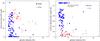 |
Fig. 1 Number of encounters with Jupiter (left panel) and the minimum distance to the planet (right panel), as a function of the aphelion distance, for NEJFCs and NEAs in cometary orbits. |
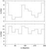 |
Fig. 2 Histogram of the argument of perihelion ω for NEJFCs (top panel) and NEAS in cometary orbits (bottom panel) at the discovery epoch. |
We found some striking features: a sharp minimum of at the discovery epoch and a noticeable past-future asymmetry, meaning that there was a larger number of comets with greater q in the past than in the future. A minimum close to the present epoch and the past-future asymmetry of have already been noticed by Fernández (1985) and Tancredi & Rickman (1992). According to Fernández (1985), the minimum at the discovery time could be attributed to an observational bias, since comets tend to be discovered when they get small-q orbits. Karm & Rickman (1982) studied the pre-discovery encounters of JFCs with Jupiter and found a remarkable tendency for close encounters to occurre right before their discovery. We also find that the mean experiences a very steep drop before the discovery time. If we consider the median of q instead of the mean, we still find an asymmetry, but the profile is flattened: the median is ~1.4 AU at –1000 yr and ~1.2 AU at +1000 yr. The fact that the asymmetry is greatly enhanced when we consider the mean, mainly in the pre-discovery branch, indicates that there is a fraction of comets coming from orbits with large q that greatly increases the dispersion.
Tancredi & Rickman (1992) studied the orbital evolution of a sample of JFCs over a time interval of 2000 yr centred on the present epoch. They also analysed the statistics of orbital evolution and the correlation with physical parameters or discovery circumstances. They confirmed the minimum of at the present epoch and the past-future asymmetry of the time evolution found by Fernández (1985), not only in but also in the averaged semimajor axis a, eccentricity e, and inclination i. This was an expected result, since these orbital elements are not independent, not only due to the obvious relation between a, e, and q, but also due to the quasi-invariance of the Tisserand parameter, which relates i to a (or q), and e.
Figure 3 also shows the evolution of the mean perihelion distance for the selected sample of NEAs in cometary orbits. As we pointed out before, there are noticeable differences with respect to the evolution of for the NEJFCs. For instance, the minimum at the discovery time is not sharply defined as in the case of NEJFCs and the curve is nearly symmetrical, leaving aside some random fluctuations. Besides, the NEA curve is practically flat in comparison to that of the NEJFCs’ curve; its amplitude is less than 0.1 AU (while the amplitude of the NEJFC curve is about 0.8 AU). The faster dynamical evolution of NEJFCs, as compared to the much quieter evolution of NEAs in cometary orbits, can be attributed to the larger number of close encounters with Jupiter and to much closer distances to the planet, as shown in Fig. 1.
We also investigated the effect of nongravitational forces in the evolution of for the studied sample of NEJFCs. Only 16 comets from this sample have computed nongravitational parameters for an epoch close to the discovery time, according to Marsden & Williams (2008). We found that the main features of the asymmetry showed in Fig. 3 were held (i.e. the sharp decrease of to the minimum at discovery time and its subsequent slower growth). Both curves for (i.e. without and with ng effects) practically overlap in the interval ~[–600, 300] yr. From ~–600 yr backwards to –1000 yr, the branch of the evolution curve varies very little (just a few hundredths of AU at its maximum difference), but the future branch starts to diverge from ~300 yr onwards, reaching a maximum difference of about 0.15 AU at 1000 yr. To see if this was due to a systematic effect introduced by ng forces, we analysed the individual evolution of q for each of the 16 comets with known ng parameters, comparing in each case the pure gravitational model against the gravitational plus ng forces. We found that the differences between the pure gravitational and the gravitational plus ng evolution of q vary randomly. We conclude that the ng forces do not significantly affect the main features of the asymmetry shown in Fig. 3 and only add a random noise to the observed evolution. By extension, we can also say that the uncertainties in the computed orbital parameters of our sample of JFCs will add some noise in our results, but their main features remain unchanged.
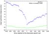 |
Fig. 3 Mean perihelion distance as function of time for the studied samples of 54 NEJFCs and 113 NEAs in cometary orbits. |
4.2. Simulations with clones of NEJFCs
We performed numerical integrations of fictitious comets, generated from the observed sample of NEJFCs. The 540 clones (ten for each comet) were obtained by varying the mean anomaly in the interval [0, 2π] at the discovery time with a uniform random distribution. The remaining orbital elements were the same as those of the comet at the discovery epoch. In this way, we randomise the orbital positions of the real comets, and thereby the fictitious comets “forget” the information about the encounters they suffered with the planets (particularly with Jupiter) because of the different geometries generated as compared to those of the real comets. We integrated in time this sample of fictitious comets in the same way that we integrated the observed NEJFCs. Figure 4 shows the resulting curve of 535 clones (five were ejected) for a time interval of 2000 yr, centred on t = 0 (namely, the normalized discovery time of each comet). This curve is practically symmetrical and, in spite of a well-defined minimum at the discovery time, the pre-discovery branch does not show the steep drop towards the minimum that the original NEJFC curve does (which is superposed to highlight the stark differences).
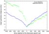 |
Fig. 4 Mean perihelion distance as a function of time for a sample of 535 clones of the studied sample of NEJFCs. For comparison purposes, the mean perihelion distance as a function of time for the sample of 54 observed NEJFCs is superimposed. |
Finally, we integrated in time a sample of 4000 fictitious comets over a period of 20 000 yr. The initial conditions for this sample were obtained in the following way: we integrated backwards (starting from the discovery epoch) the original sample of observed NEJFCs until they reached a perihelion distance greater than 2 AU, or a time limit of 2000 yr. A total of 40 comets reached q > 2 AU in the considered interval. Then we recorded the final planetary configuration and orbital elements for each of these comets (we used a time bin of 1 yr). Finally, 100 fictitious comets were generated for each of the 40 real comets as explained before, i.e. by randomly varying the mean anomaly in the interval [0, 2π], but keeping the orbital elements of the computed comet orbits at the end of the backward integration. We obtained a total number of 4000 clones in this way. The initial planetary configuration for each set of 100 clones was the same as the recorded configuration for the “parent” comet. Once the initial conditions for the fictitious comets and their corresponding planetary configurations were set, we integrated the clones for 20 000 yr forwards. During the integration, a total number of 316 clones resulted ejected (i.e. they reached a heliocentric distance above 100 AU).
We define a crossing to be when the comet perihelion distance decreases below a given threshold qthre. We assume a canonical value of qthre = 1.05 AU, based on the observed curve (cf. Fig. 3), that reaches a minimum at 1.02 AU. From the sample of 4000 clones, a number of 1179 experienced at least one crossing. To define a second, third, fourth (and so on) crossing, we imposed the condition that after a given crossing, the clone first raised its perihelion distance to above 1.3 AU and then decreased it again below qthre.
Figure 5 (top panel) shows the resulting profile, over a period of 2000 yr centred on the discovery time by assuming that a test comet is discovered at any random time when its perihelion distance q < qthre. These random times are determined in the following way: for each clone, we randomly extract a time value t from the integration time interval (more precisely from the interval [1000, 19 000] yr) until we find a time t for which q(t) < qthre (for each clone, we make a maximum number of 1000 trials to find a t that fulfills the requirement). As can be seen at the top panel of Fig. 5, neither the asymmetry nor the steep drop towards the minimum are reproduced under these discovery conditions. The resulting profile is more or less symmetrical, with a slight increase at the end of the post-discovery branch. We performed several runs in order to assess the robustness of these results.
However, when we assume that the fictitious comets are discovered at the first crossing, we are able to roughly reproduce the main features of the evolution of showed in Fig. 3: we reproduce not only the asymmetry and the minimum but also the sudden drop towards the minimum, as shown in the bottom panel of Fig. 5. When we changed the threshold to a different value with respect to the canonical one, e.g. to qthre = 1.3 AU, the resulting profile also reproduced the main features of the observed profile, though it shifted to somewhat larger values. To test the robustness of our results, we repeated the previous analysis with two subsamples, each including 2000 clones. We did not find any meaningful difference with respect to the corresponding profiles based on the entire sample.
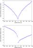 |
Fig. 5 Simulated evolution of |
To investigate the primary causes of the asymmetry showed in the bottom panel of Fig. 5, we made a quick inspection by eye of the q evolution for each clone over the 20 000 yr integration interval. To simplify the procedure, we considered only those clones with crossing times ≥1000 yr (908 clones), i.e. we left aside 271 clones that crossed the threshold qthre before 1000 yr. At first glance, we could distinguish three types of dynamical behaviour: some clones reached their first crossing after a steep fall from q > 2 AU, either starting directly from the beginning of the integration or after spending a relatively long stay in the q > 2 AU zone (we define these two kinds of behaviours as types I and III, respectively), while the remaining clones reached their first crossings after a smooth decrease of their perihelion distances spending a minimum of 3000 yr in the q < 2 AU region (this will be called type II behaviour). About two-thirds of the clones were classified as types I or III and the rest as type II. Figure 6 shows examples of each type of dynamical evolution. The clones of types I and III seem to contribute mostly to the past-future asymmetry shown in the bottom panel of Fig. 5.
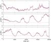 |
Fig. 6 Some examples of the different dynamical behaviours as defined in the text: perihelion distance as a function of time for a clone of comet 6P (top panel) and two clones of comet 3D (middle and bottom panels). The top panel shows an example of type I, while examples of types II and III are shown in the middle and bottom panels, respectively. The horizontal dashed line indicates the threshold of 1.05 AU. |
As a byproduct of the study of the clones during 20 000 yr, we made an estimate of the half-life of the clones keeping short-period orbits (P < 20 yr) with q < 2 AU, which was found to be about 2.4 × 10⁴ yr. This is in rather good agreement with Levison & Duncan (1994), who estimated an overall dynamical lifetime of 4.5 × 10⁵ yr for JFCs of all qs. The authors found that JFCs spend ~7% of this time with q < 2.5 AU, i.e. about 3.15 × 10⁴ yr, which is consistent with a lifetime of 2.4 × 10⁴ yr with q < 2 AU.
Figure 7 shows the profiles obtained by assuming that the comets are discovered at the start of their first, second, third, fourth, fifth, or sixth crossings. In order to compute the mean perihelion distance over a period of 2000 yr centred on the first crossing time for those clones with a crossing time <1000 yr, we integrated their orbits (in time) until completing 1000 yr backwards. As we can show in the figure, as the order of the crossing increases, the past and future branches tend to flatten and, after the third crossing, the asymmetry tends to reduce and even reverse the greater slope from the pre- to the post-discovery branch. By contrast, the observed profile of shows a strong asymmetry (cf. Fig. 3), so we can infer that very few comets are discovered after a second crossing, since otherwise we would observe a flatter and more symmetrical profile. The average times of the clones to reach the first, second, and third crossings are found to be 5500, 7400, and 8800 yr, respectively. However, standard deviations are 5200, 5100, and 4700 yr respectively. Then, the median would be a better estimation than the mean for the half time of each crossing. The median times to reach the first, second, and third crossings are found to be 3700, 6500, and 8700 yr, respectively. If we assume an orbital period of 6 yr estimated from the mean orbital period of the observed NEJFC sample, then the median times to reach the first, second, and third crossings would be approximately 600, 1100, and 1450 revolutions, respectively.
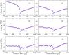 |
Fig. 7 Simulated evolution of |
Figure 8 shows some theoretical profiles compared to the observed one. The simulated profiles were obtained by assuming that the comets were discovered when their perihelia crossed the threshold at 1.05 AU for the first time and that a certain fraction F of the comets were of type II (and the remaining of types I and III). The sample was drawn from test comets randomly extracted from the 254 clones of type II and from the 575 clones of types I and III. We left aside 79 clones that crossed after 1000 yr, but did not fit well to any dynamical type. To allow for a certain degree of randomness, we constrained the size of the type II sub-sample to 50% of the original one. The figure shows three examples of the theoretical curves obtained for three different fractions F: 0.3 (top panel), 0.6 (middle panel), and 0.8 (bottom panel). As the fraction of type II comets increases, the simulated curve tends to flatten and then to reduce the asymmetry. The number of comets included in the sample for each of the simulated curves varies with the parameter F (since the number of type II comets was taken as a fixed quantity, i.e. 127, while the number of type I and III comets was adjusted in each case to the fraction 1-F). Thus, the sample for the first curve (top panel) includes 406 comets, the sample for the second curve (middle panel) considers 213 comets, and the sample for the third curve (bottom panel) comprises 151 comets. The best-fit parameter was F ~ 0.6, i.e. about 60% of the fictitious NEJFCs were of type II, while about 40% were of types I or III. The latter can be related to young, fresh comets coming straight from orbits with q > 2 AU, while the former can be related to older, more evolved comets that have spent ≳3000 yr with q < 2 AU, according to our definition of each type.
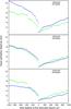 |
Fig. 8 Some theoretical curves |
4.3. Physical lifetime of NEJFCs
As a corollary to this work we can estimate lower and upper limits for the median physical (i.e. active) lifetime τphys of NEJFCs in the q < 2 AU region, based on our theoretical fits to the observed profile (cf. Fig. 8). We can set an upper limit to the NEJFCs τphys of about half the dynamical time scale of JFCs with q < 2 AU, i.e. about 10 000–12 000 yr, or equivalently of about 1600–2000 revolutions, since otherwise, for longer discovery time scales, most comets would be discovered during the fourth or later crossings, which, as we saw (cf. Fig. 7) would produce fairly symmetrical profiles. We can also set a lower limit by considering the minimum time that a comet requires to reach its first crossing. This would be typically several hundred years (~100 revolutions).
5. Discussion
Fernández (1985) estimated the physical lifetime of the JFCs by assuming a balance between comet gains and losses and a certain transfer rate of JFCs to the region of the terrestrial planets. He derived an average physical lifetime of about 1000 revolutions for a typical kilometer-sized JFC with q ~ 1 AU, which actually can be regarded as an upper limit. Other estimates of the physical lifetime of JFCs, constrained to the q < 1.5 AU region, are 400 revolutions (Kresák 1981), 300 revolutions (Kresák & Kresáková 1990), 200 revolutions (Emel’yanenko et al. 2004), and 150−200 revolutions (di Sisto et al. 2009). Levison & Duncan (1997) estimated a physical lifetime of 600 revolutions for JFCs without constraints on q. As compared to the previous authors, our estimated physical lifetime is for a somewhat larger q (<2 AU) population. The upper limit of ~104 yr (or 1600–2000 revolutions) is still consistent with the previous estimates, though somewhat longer.
As we can see in the top panel of Fig. 5, the evolution of around random discovery times for the fictitious comets is practically symmetrical. This is an easily understood result, since once the orbital elements of the clones (actually, it was enough to randomize the mean anomaly) were randomised, the memory of the evolution of the real comets is lost. The lack of the main features shown by the observed NEJFCs’ evolution of (i.e. the remarkable past-future asymmetry and the sudden drop to the minimum at discovery time) in the clones’ evolution of suggests that those features may be attributed to some bias that favors the discovery of the NEJFCs, when their q is decreasing fairly steadily. Comet 72D/Denning-Fujikawa is a good example of those comets that contribute to the observed past-future asymmetry (cf. top panel of Fig. 3). According to our integrations, this comet would have been a Centaur until it changed its semimajor axis from ~12 AU to less than 6 AU approximately 400 years before its discovery. This was due to a very close encounter with Saturn that turned it into a JFC. The gap of about 0.1 AU, which can be observed at approximately –400 yr in the NEJFCs’ profile of Fig. 3, is due to this comet, which shows a fast decrease of its perihelion distance, from values of q > 2 AU, prior to its discovery.
5.1. An estimate of τphys based on the sublimation lifetime
To analyse if our estimated physical lifetime is consistent with other physical features of comets, we assume that the cometary lifetime is set by the mass loss due to sublimation of water ice. The sublimation lifetime τphys,subl (in number of revolutions) of a free-sublimating comet nucleus is given by (Fernández 2005)  (2)where RN is the radius of the comet nucleus and Δh is the thickness of the sublimated outer layer per orbital revolution, which is related to the bulk density ρN of the nucleus and to the mass loss Δm per unit area and per orbital revolution of the nucleus by means of
  (3)The mass loss Δm can be computed from the polynomial fit given by di Sisto et al. (2009) to theoretical thermodynamical models of a free-sublimating comet nucleus:
  (4)where q is given in AU and Δm in g cm-2. We can introduce a correcting factor in the computation of τphys,subl to account for a certain fraction f of active surface area. By assuming f = 0.1, the corrected sublimation lifetime would be
  . Then, for a NEJFC of q = 1.5 AU, ρN = 0.4 g cm-3, and RN = 1 km, we would have a sublimation lifetime of about 6950 revolutions. Strictly speaking, this value should be taken as an upper limit since comets are subject to frequent outbursts and splittings (e.g. Chen & Jewitt 1994) with greatly enhanced mass loss. Bearing this in mind, we can say that a physical lifetime of ~1000 revolutions is consistent with the estimated mass loss by sublimation, outbursts, and splittings.
5.2. An estimate of τphys based on the extinct JFCs
We can also try to estimate the physical lifetime of JFCs τphys,ext based on the size n of the population of observed JFCs with q < 2 AU and on the extinction rate ṅext of this population by means of  (5)where the extinction rate can be estimated from the known JFCs that are assumed to have become extinct. In the Marsden & Williams (2008) catalogue, there are several comets indicated with a D (standing for disappeared) though they might be still around and active. Strictly speaking, they have been missed for several apparitions, though that does not necessarily imply that they are extinct. The rediscovery of several of them, D/1896 R2 (205P/Giacobini), D/1892 T1 Barnard 3 (206P/Barnard-Boattini), and D/1783 W1 Piggot (226P/Piggot-LINEAR-Kowalski), gives support to the idea that all or most of them might still be active. Among the most firm candidates to have become currently extinct, we have 3D/Biela (split in 1846, not seen since then), 5D/Brorsen (not seen since 1879, despite very favorable returns), 25D/Neujmin 2 (not seen since 1927, despite very favorable returns), 18D/Perrine-Mrkos (showed large brightness fluctuations and erratic nongravitational effects, last seen in 1968 when it was very faint, 12m, probably extinct), and 34D/Gale (not seen since 1938, very faint object, it could be extinct, see a discussion by Kresák 1981). D/1819 W1 Blanpain is another good candidate. The NEA 2003 WY25 may be associated to this comet. According to Jewitt (2006), its radius was estimated to be 160 m and showed residual activity, so it may be a fragment of the disintegration of the comet. We conclude that the extinction rate of JFCs with q < 2 AU may be at most 2–3 comets century-1.
By substituting ṅext = 2.5 comets century-1 and assuming n ~ 200, from Eq. (5) we see that the physical lifetime based on the extinction rate would be τphys,ext ≃ 80 centuries = 8000 yr (≃ 1300 revolutions), which is consistent with our estimated physical lifetime.
6. Concluding remarks
We studied the dynamical evolution of JFCs that come close to the Earth and compared it with that of NEAs. We were able to reproduce fairly well the time evolution of the mean perihelion distance of the NEJFCs and, as a byproduct, put some constraints on the physical lifetime of this population of short-period comets. Our main conclusions are the following:
-
We confirm a well-defined minimum of the mean perihelion distance
of the NEJFCs at discovery time and a remarkable past-future asymmetry in the [–1000, +1000] yr interval centred on the discovery time of each comet. The asymmetry means that there are more comets with greater q in the pre-discovery branch than in the post-discovery branch. We also find a very steep drop of towards the minimum at the discovery time (assumed to be t = 0 for all comets). Since the median of q appears more flattened, we conclude that the past-future asymmetry is mainly due to some comets that decrease their perihelia very fast from the q > 2 AU region, until they are discovered. -
We found some remarkable differences in the dynamical evolution of NEJFCs and NEAs in cometary orbits. For instance, the evolution of
for NEAs in cometary orbits is practically flat and symmetrical, as compared to that for NEJFCs. The flatness can be attributed to a more quiet dynamical evolution since NEAs experience on average less close encounters with Jupiter, as compared to NEJFCs. The symmetry would be because NEAs can be discovered at any time during their evolution, even after a long stay in the q < 1.3 AU region, since their lifetimes are dynamical, not physical, with a median dynamical time scale of ~10 Myr (Gladman et al. 2000). In addition, the argument of the perihelion ω of NEJFC clusters around ω ~ 0° and ω ~ 180° as expected, while NEAs in cometary orbits (with H < 18) show fairly uniform distribution in ω. These significant differences in the dynamical evolution argues against a common origin for both populations, in which the NEAs in cometary orbits were assumed to be dormant or extinct comets. We conclude that some of the differences in the dynamical evolution of both populations would be due to their different physical nature, meaning that the lifetimes of NEAs are just dynamical, while for NEJFCs the physical lifetimes are relevant. -
By assuming that NEJFCs are mostly discovered during their first crossing (i.e. when they decrease their perihelion distance below a certain threshold qthre = 1.05 AU for the first time during their evolution in the q < 2 AU region), we are able to reproduce the main features of their observed
evolution in the interval [–1000, 1000] yr with respect to the discovery time. We reproduce not only the asymmetry and the minimum but also the sudden drop towards the minimum. The fact that comets would be mostly discovered during their first crossing is consistent with the fragile structure and icy composition of the cometary nucleus, which are reflected in a short physical lifetime. As with the observed evolution of NEAs in cometary orbits, when we allow the fictitious NEJFCs to be discovered at any random time t with q(t) < qthre, neither the asymmetry nor the steep drop towards the minimum in the profile is reproduced. -
Our best fits to the observed
profile of the NEJFCs indicate that ~40% of this population would be composed of young, fresh comets that entered the region q < 2 AU a few hundred years before their perihelion distances fell below qthre, while ~60% would be composed of older, more evolved comets, discovered after spending at least ~3000 yr in the q < 2 AU region. -
According to what was reported above, if the NEJFCs had lifetimes set by their dynamics (which we estimate to be around 24 000 yr), their
profile around the discovery time should be symmetrical like the one showed by NEAs in cometary orbits. Since the NEJFC profile is noticeable asymmetrical, NEJFCs should have a physical lifetime significantly shorter than their dynamical one, say less than a half of that. This will allow comets to be largely discovered at their first or second crossing at most. We estimate lower and upper limits for the physical lifetime τphys of NEJFCs in the q < 2 AU region, based on the comparison between the NEJFC profile and the theoretical profile for first crossings. We set a lower limit of several hundred years and an upper limit of about 10 000–12 000 yr, or about 1600–2000 revolutions. Probably a typical JFC will last several 103 yr (or about 103 revolutions) in this region. These constraints are consistent with other estimates of τphys, based either on mass loss (sublimation, outbursts, splittings) or on the extinction rate of JFCs.
Acknowledgments
A.S. acknowledges the Comisión Sectorial de Investigación Científica, Universidad de la República, for their financial support for this work, which is part of her Ph.D. Thesis at the Universidad de la República, Uruguay. We also thank the anonymous referee for a careful reading of the manuscript.
References
- Binzel, R. P., Xu, S., Bus, S. J., & Bowell, E. 1992, Science, 257, 779 [NASA ADS] [CrossRef] [Google Scholar]
- Carusi, A., Kresak, L., Perozzi, E., & Valsecchi, G. B. 1987, A&A, 187, 899 [NASA ADS] [Google Scholar]
- Chambers, J. E. 1999, MNRAS, 304, 793 [NASA ADS] [CrossRef] [MathSciNet] [Google Scholar]
- Chen, J., & Jewitt, D. 1994, Icarus, 108, 265 [NASA ADS] [CrossRef] [Google Scholar]
- di Sisto, R. P., Fernández, J. A., & Brunini, A. 2009, Icarus, 203, 140 [NASA ADS] [CrossRef] [Google Scholar]
- Emel’yanenko, V. V., Asher, D. J., & Bailey, M. E. 2004, MNRAS, 350, 161 [NASA ADS] [CrossRef] [Google Scholar]
- Fernández, J. A. 1985, Icarus, 64, 308 [NASA ADS] [Google Scholar]
- Fernández, J. A. 2005, Comets: Nature, Dynamics, Origin, and Their Cosmogonical Relevance, ASSL 328 (Springer-Verlag) [Google Scholar]
- Fernández, J. A., Gallardo, T., & Brunini, A. 2002, Icarus, 159, 358 [NASA ADS] [CrossRef] [Google Scholar]
- Fernández, Y. R., Jewitt, D. C., & Sheppard, S. S. 2005, AJ, 130, 308 [NASA ADS] [CrossRef] [Google Scholar]
- Gladman, B., Michel, P., & Froeschlé, C. 2000, Icarus, 146, 176 [NASA ADS] [CrossRef] [Google Scholar]
- Jewitt, D. 2006, AJ, 131, 2327 [NASA ADS] [CrossRef] [Google Scholar]
- Karm, J., & Rickman, H. 1982, Bull. Astr. Inst. Czechosl., 33, 359 [NASA ADS] [Google Scholar]
- Kresák, L. 1981, Bull. Astr. Inst. Czechosl., 32, 321 [Google Scholar]
- Kresák, L., & Kresáková, M. 1990, Icarus, 86, 82 [NASA ADS] [CrossRef] [Google Scholar]
- Levison, H. F., & Duncan, M. J. 1994, Icarus, 108, 18 [NASA ADS] [CrossRef] [Google Scholar]
- Levison, H. F., & Duncan, M. J. 1997, Icarus, 127, 13 [Google Scholar]
- Marsden, B. G., & Williams, G. V. 2008, Smithsonian Astrophysical Observatory, Cambridge, MA [Google Scholar]
- Marsden, B. G., Sekanina, Z., & Yeomans, D. K. 1973, AJ, 78, 211 [NASA ADS] [CrossRef] [Google Scholar]
- Tancredi, G., & Rickman, H. 1992, in Chaos, Resonance, and Collective Dynamical Phenomena in the Solar System, ed. S. Ferraz-Mello, IAU Symp., 152, 269 [Google Scholar]
- Wetherill, G. W. 1991, in Comets in the post-Halley era, eds. R. L. Newburn, Jr., M. Neugebauer, & J. Rahe, IAU Colloq., 116, Astrophys. Space Sci. Lib., 167, 537 [Google Scholar]
All Tables
All Figures
|
Fig. 1 Number of encounters with Jupiter (left panel) and the minimum distance to the planet (right panel), as a function of the aphelion distance, for NEJFCs and NEAs in cometary orbits. |
| In the text | |
|
Fig. 2 Histogram of the argument of perihelion ω for NEJFCs (top panel) and NEAS in cometary orbits (bottom panel) at the discovery epoch. |
| In the text | |
|
Fig. 3 Mean perihelion distance as function of time for the studied samples of 54 NEJFCs and 113 NEAs in cometary orbits. |
| In the text | |
|
Fig. 4 Mean perihelion distance as a function of time for a sample of 535 clones of the studied sample of NEJFCs. For comparison purposes, the mean perihelion distance as a function of time for the sample of 54 observed NEJFCs is superimposed. |
| In the text | |
|
Fig. 5 Simulated evolution of |
| In the text | |
|
Fig. 6 Some examples of the different dynamical behaviours as defined in the text: perihelion distance as a function of time for a clone of comet 6P (top panel) and two clones of comet 3D (middle and bottom panels). The top panel shows an example of type I, while examples of types II and III are shown in the middle and bottom panels, respectively. The horizontal dashed line indicates the threshold of 1.05 AU. |
| In the text | |
|
Fig. 7 Simulated evolution of |
| In the text | |
|
Fig. 8 Some theoretical curves |
| In the text | |
Current usage metrics show cumulative count of Article Views (full-text article views including HTML views, PDF and ePub downloads, according to the available data) and Abstracts Views on Vision4Press platform.
Data correspond to usage on the plateform after 2015. The current usage metrics is available 48-96 hours after online publication and is updated daily on week days.
Initial download of the metrics may take a while.