| Issue |
A&A
Volume 548, December 2012
|
|
|---|---|---|
| Article Number | A121 | |
| Number of page(s) | 25 | |
| Section | Extragalactic astronomy | |
| DOI | https://doi.org/10.1051/0004-6361/201219751 | |
| Published online | 04 December 2012 | |
Modeling optical and UV polarization of AGNs
II. Polarization imaging and complex reprocessing
1
Observatoire Astronomique de Strasbourg, Université de Strasbourg, CNRS,
UMR 7550, 11 rue de l’Université,
67000
Strasbourg,
France
e-mail: This email address is being protected from spambots. You need JavaScript enabled to view it.
2
Centro de Astrofísica de Valparaíso y Departamento de Física y
Astronomía, Universidad de Valparaíso, Av. Gran Bretaña 1111, Valparaíso, Chile
3
Astronomical Institute of the Academy of Sciences,
Bočni II 1401,
14131
Prague, Czech
Republic
Received:
4
June
2012
Accepted:
12
September
2012
Abstract
Context. The innermost parts of active galactic nuclei (AGNs) are believed to be comprised of several emission and scattering media coupled by radiative processes. These regions generally cannot be spatially resolved. Spectropolarimetric observations give important information about the reprocessing geometry.
Aims. We aim to obtain a coherent model of the polarization signature resulting from the radiative coupling between the components, to compare our results with polarimetry of thermal AGNs, and thereby to put constraints on the geometry.
Methods. We used a new public version of stokes, a Monte Carlo radiative transfer code presented in the first paper of this series. The code has been significantly improved for computational speed and polarization imaging has been implemented. The imaging capability helps to improve understanding of the contributions of different components to the spatially-integrated flux. We coupled continuum sources with a variety of reprocessing regions such as equatorial scattering regions, polar outflows, and toroidal obscuring dust and studied the resulting polarization. We explored combinations and computed a grid of thermal AGN models for different half-opening angles of the torus and polar winds. We also considered a range of optical depths for equatorial and polar electron scattering and investigated how the model geometry influences the type-1/type-2 polarization dichotomy for thermal AGNs (type-1 AGNs tend to be polarized parallel to the axis of the torus while type-2 AGNs tend to be polarized perpendicular to it).
Results. We put new constrains on the inflowing medium within the inner walls of the torus. To reproduce the observed polarization in type-1 objects, the inflow should be confined to the common equatorial plane of the torus and the accretion disk and have a radial optical depth of 1 < τ < 3. Our modeling of type-1 AGNs indicates that the torus is more likely to have a large (~60°) half-opening angle. Polarization perpendicular to the axis of the torus may arise at a type-1 viewing angle for a torus half-opening angle of 30°–45° or polar outflows with an optical depth near unity. Our modeling suggests that most Seyfert-2 AGN must have a half-opening angle >60° to match the expected level of perpendicular polarization. If outflows are collimated by the torus inner walls, they must not be optically thick (τ < 1) to preserve the polarization dichotomy. Then, varying the wind’s optical depth does not affect the degree of polarization of type-2 thermal AGNs but it has a significant impact on the type-1/type-2 polarization dichotomy when τ > 0.3.
Key words: galaxies: active / galaxies: Seyfert / polarization / radiative transfer / scattering
© ESO, 2012
1. Introduction
Active galactic nuclei (AGN) are divided observationally into a number of (sub-)classes based on the optical spectrum and radio properties. If the broad-line region (BLR) is directly visible in the optical, the AGN is of type-1, while if the BLR is not visible, it is of type-2. The AGNs can also be divided into “radio-loud” and “radio-quiet” AGN, depending on the relative strength of the kpc-scale radio jets and lobes.
Blandford & Rees (1978) suggested that BL Lac objects were radio-loud AGNs, whose jets are aimed close to our line of sight. Keel (1980) discovered that nearby type-1 AGNs are preferentially oriented face-on while nearby type-2 AGNs are randomly oriented. These discoveries showed that the viewing angle of the observer is a key element in AGN classification (Antonucci 1993). The apparent absence of a BLR in type-2 AGNs is explained by a dusty medium that hides the BLR at certain viewing angles from the observer. The ionizing continuum source and its surrounding BLR sit inside the funnel of the torus. In this scenario the half-opening angle of the torus can be estimated from the ratio of type-1 to type-2 AGNs in an isotropically selected sample and from the “infra-red calorimeter” – the relative strength of the mid-IR continuum that arises from dust reprocessing of the higher-energy continuum (see Antonucci 2012). There is evidence that the opening angle is a function of luminosity (Lawrence 1991) or accretion history (Wang & Zhang 2007).
The distinction between radio-loud and radio-quiet objects is orientation-dependent and therefore cannot be explained as a geometry effect. Furthermore, it has been argued by Antonucci (2012) that there is a fundamental difference in the dominant energy generation between high-accretion-rate sources, which are believed to release the bulk of their radiated energy via thermal disk emission in the far-ultraviolet (see Gaskell 2008) and low-accretion-rate AGNs, which are dominated by nonthermal emission. The latter class of AGNs includes the so-called “naked” AGNs (Georgantopoulos & Zezas 2003; Gliozzi et al. 2007; Bianchi et al. 2008)1. The transition between the two modes of dominant energy generation take place at an Eddington ratio of ~10-3 (Antonucci 2012). Following Antonucci (2012), we refer to these two types of AGNs as “thermal AGNs” and “nonthermal AGNs”, respectively2. The thermal/nonthermal dichotomy is the causal consequence of the accretion mode (related to the accretion rate) that has an impact on the accretion disk and thus on the eventual observation of its thermal emission. By definition, thermal AGNs always have a big blue bump. As far as is known (see Antonucci 2012), they also always have a BLR, although the BLR might be hidden, as in type-2 AGNs3. Nonthermal AGNs are Fanaroff-Riley (FR) I radio galaxies and Low-ionization nuclear emission-line regions (LINERs). It is important to note that the thermal/nonthermal distinction is not the same as the radio-quiet/radio-loud distinction. A radio-loud AGN can be either a thermal AGN (for example, 3C 273) or a nonthermal AGN (such as M 87). For completeness we also point out that optically violently variable (OVV) behavior in blazars can arise from both thermal and nonthermal AGNs. However we consider here the AGN with a jet aimed close to our line of sight. We do not consider blazars here because of the strong intrinsic polarization of the synchrotron emission in the jets.
In this work, we focus on polarization modeling of radio-quiet AGNs that release the bulk of their radiated energy in the far UV. Our goal is to infer clues about the geometry and composition of the different AGN components from the observed polarization properties. We assume that in thermal AGNs the emission comes from an optically thick accretion disk (Lynden-Bell 1969). Closely associated with the accretion disk, and occupying approximately the same range of radius, is the BLR – a supposedly flattened region of high-density (ne ~ 1010 cm-3), rapidly moving (v ~ 0.05−0.001c) gas which is optically thin in the continuum for hν < 13.6 eV (see Gaskell 2009, for a review).
Not all matter that spirals into the gravitational potential of the black hole becomes accreted. In many radio-quiet AGN strong winds are seen in the X-ray and UV spectrum (Mathur et al. 1994, 1995; Costantini 2010). Supposedly, these winds are expelled very close to the black hole and find a spatial continuation in the observed polar ionization cones. In some objects the outflowing gas can be seen as broad absorption lines (Weymann et al. 1991; Knigge et al. 2008). Immediately outside the BLR and accretion disk is the geometrically thick, dusty torus (but see Elvis 2000, 2004; Kazanas et al. 2012, and references therein for the interpretation of the equatorial obscuration as a wind). Finally, starting on a scale larger than the BLR and often extending to distances much greater than the size of the torus there is the lower-density, lower-velocity gas of the so-called “narrow-line region” (NLR).
The accretion flow at the outer accretion disk and the inner boundary of the torus funnel is difficult to assess observationally. At a distance of about a thousand gravitational radii from the black hole the accretion flow should become gravitationally unstable and become fragmented (see e.g. Lodato 2007). There are indications that the medium is continuous while being inhomogeneous in density (Elitzur 2007). In this context the interaction between the primary radiation from the accretion disk with the surrounding media causes scattering-induced polarization signatures. In a single electron- or dust-scattering event, the resulting polarization degree and position angle depend on the scattering angle, and therefore the resulting net polarization of the collective reprocessing in an AGN, when accurately modeled, allows us to draw conclusions about the geometry of the scattering regions. Some evidence for a flattened geometry of the matter just inside the torus comes from optical polarimetry. For many type-1 objects the E-vector of the continuum radiation aligns with the projected axis of the (small-scale) radio structures (Antonucci 1982, 1983). Identifying the radio structures with collimated outflows progressing along the symmetry axis of the dusty torus, such a polarization state is most easily explained by scattering in a flattened, equatorial scattering region (Antonucci 1984). The polarization state of the radiation thus brings information about the reprocessing geometry. Based on an analysis of the polarization structure across broad emission lines, Smith et al. (2004) suggested that the equatorial scattering region may be partly intermixed with or lie slightly farther out than the BLR.
This is the second paper of a series in which we systematically examine the polarization response caused by combining different scattering regions. We built models of double-component AGNs, i.e. “naked”, “bare”, FR I, or LINERs-like galaxies to then present a multi-component model for thermal AGNs and examine how the polarization spectra and images are influenced by the different AGN constituents. We applied the latest publicly available version 1.2 of the radiative transfer code stokes. Source codes, executables, and a manual of stokes 1.2 can be found on the internet4.
The remainder of the paper is organized as follows: in Sect. 2 we briefly summarize our previous modeling work on AGN and describe the new elements of stokes 1.2. In Sect. 3, polarization images for individual AGN scattering regions are studied. Consistent models for combining two scattering regions are presented in Sect. 4 and a three-component model approximating the unified AGN model is explored in Sect. 5. In Sect. 6 we discuss our results and relate them to the work done by other groups before we draw our conclusions in Sect. 7.
2. Applying the radiative transfer code STOKES
In Goosmann & Gaskell (2007, hereafter Paper I), we published polarization modeling for reprocessing by different individual scattering components. In Paper I we studied centrally illuminated dusty tori, polar outflows, and equatorial scattering regions with different geometries. The spectral flux and polarization were computed and discussed in the context of observed spectropolarimetric data and of the modeling work done by other groups. In our subsequent work, we have explored the polarization induced by different dust compositions in the torus or the polar outflow (Goosmann et al. 2007a,b), compared two competitive scenarios to explain the emergence of the broad Fe Kα line in the Seyfert 1 galaxy MCG-6-30-15 (Marin et al. 2012b), investigated time-dependent polarization due to reverberation (Goosmann et al. 2008; Gaskell et al. 2012), and investigated the effect of an inflow velocity of the scattering medium on the shape of AGN emission lines (Gaskell & Goosmann 2008).
In these studies we focused on the effects of single scattering regions. It is important to consider the effects of combined scattering regions. For example, by putting together a dusty torus, ionized polar outflows, and equatorial scattering it is possible to reproduce the observed dichotomy of the polarization position angle between type-1 and type-2 AGN (Goosmann 2007) and even to derive predictions for this dichotomy in the X-ray range (Marin & Goosmann 2011; Marin et al. 2012a). In the present paper, we therefore systematically investigate the polarization due to scattering in various combinations of reprocessing regions. We use the latest publicly available version, stokes 1.2, of our radiative transfer code. In this section, we describe the most significant improvements and changes made with respect to the previous version stokes 1.0.
2.1. Improved random number generator
The standard deviation of a Monte Carlo calculation is usually proportional to the square root of the number of samples. In radiative transfer modeling, enough photons need to be sampled to suppress the Poisson noise with respect to significant spectral or polarization features. In many of the models shown below we therefore sampled 109 photons or more. The generation of such long series of random numbers may run into numerical problems. In stokes 1.0 a linear congruential generator (LCG) was used, which is fast and efficient only for short series. For the large sampling numbers that are typically applied in the complex modeling presented here, the LCG tends to loop back on series of values it has sampled before. In stokes 1.2, we therefore implemented a version of the Mersenne twister generator (MTG) algorithm (Matsumoto & Nishimura 1998). The MTG generates pseudo-random numbers using a so-called twisted generalized feedback shift register. The most common version, MT 19937, has a very high period of 219937 − 1 and provides a 623-dimensional equidistribution up to an accuracy of 32 bits. The MTG is more efficient than most other random number generators and passes the “Diehard” tests described in Marsaglia (1985). A detailed analysis of the MTG is given in Matsumoto & Nishimura (1998) and references therein. Using the MTG in stokes substantially improves the statistics for a given sampling number of photons. Although each call of the MTG requires 20% more computation time compared to the LCG, far fewer photons are needed to obtain the same limit on the Poissonian fluctuations. Therefore, there is a significant net gain in computation time and the results converge faster.
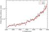 |
Fig. 1 Modeling a central, isotropic source that irradiates a dusty, equatorial scattering torus with a half-opening angle of 30° (see text). The spectrum represents the polarized flux, PF/F∗, normalized to the source flux F∗, for a viewing angle of i = 72°. The spectra were calculated by sampling the same number of photons but using two different random number generators. Black dashed line: the LCG algorithm as implemented in stokes 1.0; red solid line: the MTG algorithm as implemented in stokes 1.2. |
We show a comparison of both methods in Fig. 1. We modeled an AGN obscuring torus sampling a total of 3 × 10⁸ photons, alternately using the LCG random number generating algorithm of stokes 1.0 and the MTG algorithm implemented in stokes 1.2. We assumed a large, dusty torus with an elliptical cross-section, constant density, and a V-band optical depth of τV ~ 600. The half-opening angle of the scattering region with respect to the symmetry axis of the torus equals θ0 = 30°. The dust has a Milky Way composition (see Sect. 4.2 of Paper I for more details). We chose this model to illustrate the effects of the random number generator because the spectra suffer from heavy absorption and only multiply scattered photons escape from the funnel of the torus. As a result, the statistics at the particular viewing angle of i = 72° tends to be low. Figure 1 shows that, for the same number of simulated photons, the simulation using the LCG algorithm suffers from much higher Poissonian noise. To obtain a curve as smooth as the one obtained with the MTG algorithm, LCG would have generate a dozen times as many photons.
2.2. Polarization imaging
To understand scattering by various regions in AGNs (see next subsection) it is very useful to be able to see polarization maps. These can also potentially be compared with future observations. With stokes 1.2 it is now possible to generate polarization images. For this, each photon is spatially located before its escape from the modeling region and is projected onto the observer’s plane of the sky. The resulting polarization maps can be compared to polarization imaging observations of spatially resolved objects. In unresolved objects, the model images can help to study the interplay of several scattering components.
We project the position of an escaping photon onto a distant plane, D,
which is orthogonal to the line of sight (Fig. 2).
The photon position P is determined by its distance,
rp, from the origin O of the model space
and by the two angles θp and
φp. The center of the projection plane O′
is connected to O by the segment OO′, which determines the polar and azimuthal viewing
angles φ and θ. The distance between O′ and the
projected photon position P′ is denoted by the vector
 .
By expressing
in the local frame of D, we obtain the projected photon
coordinates x′ and y′ in the
plane of the sky.
.
By expressing
in the local frame of D, we obtain the projected photon
coordinates x′ and y′ in the
plane of the sky.
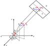 |
Fig. 2 Spatial coordinates that determine the position of a photon P and its projection P′ onto the plane of the sky, D. |
The unit vectors  and
and  are expressed in spherical coordinates:
 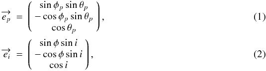 while
the unit vectors of the observer’s plane of the sky can be written as
while
the unit vectors of the observer’s plane of the sky can be written as 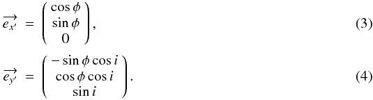 We
then construct the vector
We
then construct the vector ![Mathematical equation: \hbox{$\overrightarrow \varrho = r_p[\overrightarrow{e_p} - \cos\chi \overrightarrow{e_i}]$}](/articles/aa/full_html/2012/12/aa19751-12/aa19751-12-eq40.png) and
obtain its components in spherical coordinates:
and
obtain its components in spherical coordinates: ![Mathematical equation: \begin{eqnarray} \varrho_x &=& r_p[\sin\phi_p \sin\theta_p - \cos\chi \sin\phi \sin i ],\\ \varrho_y &=& r_p[\cos\chi \cos\phi \sin i - \cos\phi_p \sin\theta_p],\\ \varrho_z &=& r_p[\cos\theta_p - \cos\chi \cos i], \end{eqnarray}](/articles/aa/full_html/2012/12/aa19751-12/aa19751-12-eq41.png) with
χ being the angle between
and .
Using Eqs. (3) and (4), we finally obtain the projected coordinates
with
χ being the angle between
and .
Using Eqs. (3) and (4), we finally obtain the projected coordinates
 and
and  of the photon in the plane of the sky:
 ![Mathematical equation: \begin{eqnarray} x' &=& - r_p \sin\theta_p \sin(\phi-\phi_p),\\ y' &=& r_p[\sin i \cos\theta_p - \cos i \sin\theta_p \cos(\phi-\phi_p)]. \end{eqnarray}](/articles/aa/full_html/2012/12/aa19751-12/aa19751-12-eq45.png)
3. Polarization maps of individual scattering regions
In a model with multiple reprocessing components, theoretical polarization maps are very useful for understanding the impact of individual scattering regions. We first tested the new imaging routines of stokes by reanalyzing some of the individual reprocessing regions presented in Paper I. For the remainder of this paper, we define a type-1 view of a thermal AGN by a line of sight toward the central source that does not intercept the torus. In this case the viewing angle (measured from the pole) is smaller than the half-opening angle of the torus. If this is not the case, we call the source a type-2 AGN. Polarization is described as parallel when the E-vector is aligned with the projected torus axis (polarization position angle γ = 90°). Sometimes we denote the difference between parallel and perpendicular polarization by the sign of the polarization percentage, P: a negative value of P stands for parallel polarization, a positive P for perpendicular one. Finally, both the spectra and the maps will show the total (linear plus circular) polarization, P. Due to dust scattering the V Stokes parameter can be nonzero, but in all our models the circular polarization was found to be a hundred times lower than the linear polarization and thus it does not have an impact on the polarization results.
3.1. Modeling a large, dusty torus
The spectral properties of such a large, dusty scattering torus were presented in Sect. 4.2 of Paper I. For all models presented below we define an isotropic, point-like source emitting an unpolarized spectrum with a power-law spectral energy distribution F∗ ∝ ν−α and α = 1 at the center of the torus. The inner and outer radii of the torus are set to 0.25 pc and 100 pc, respectively. The radial optical depth of τV measured inside the equatorial plane is taken to be ~750 in the V-band. The half-opening angle of the torus is set to θ0 = 30° with respect to the vertical axis.
3.1.1. Wavelength-integrated polarization images
We sampled a total of 109 photons and modeled spectra and images at 20 polar viewing angles i and 40 azimuthal angles φ; i and φ are the viewing angles defined as in Fig. 2. The angle i is measured between the line of sight and the z axis; φ is measured between the projection of the line of sight onto the xy-plane and the x axis. A fairly fine stratification in viewing angle is necessary to limit the image distortion that occurs preferentially at polar angles. The meshes of the coordinate grid have a different shape at the poles, where they are more trapezium-like, than at the equator, where they are almost square-like. The spectra are presented in terms of cosi providing an equal flux per angular bin for an isolated, isotropic source located at the center of the model space. Since the model is symmetric with respect to the torus axis, we averaged all Stokes parameters over φ and thereby improve the statistics. As in Fig. 4, we will present imaging results at three different polar angles: i ~ 18° (near to pole-on view), i ~ 45° (intermediate viewing angle), and i ~ 87° (edge-on view). These lines of sight roughly represent AGN of type-1, of an intermediate type between type-1/type-2, and of type-2, respectively. We define a spatial resolution of 30 bins for the x′ and y′ axes so that the photon flux is divided into 900 pixels. Each of these pixels is labeled by the coordinates x′ and y′ (in parsecs) and stores the spectra of the four Stokes parameters across a wavelength range of 1800 Å to 8000 Å. Ultimately, each pixel contains the same type of spectral information that is provided by the previous, nonimaging version of stokes.
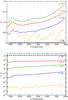 |
Fig. 3 Modeling an optically thick elliptically shaped torus with θ0 = 30° measured relative to the symmetry axis. The spatially integrated polarization P (upper panel) and the fraction F/F∗ of the central flux (lower panel) are seen at different viewing inclinations, i. |
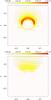 |
Fig. 4 Model image of the polarized flux, PF/F∗, for a centrally irradiated optically thick, elliptically shaped torus with θ0 = 30° measured relative to the symmetry axis; PF/F∗ is color–coded and integrated over the wavelength band. Top: face-on view at i ~ 18°; bottom: view at i ~ 45°. |
The polarization and flux spectra integrated over x′ and y′ are shown in Fig. 3. As expected, they agree with previous results (see Sect. 4.2 and Fig. 6 of Paper I for more details). The polarization images are shown in Fig. 4. Because the torus is so huge we zoomed in on the imaging and analyzed specifically the torus funnel from which the most scattered radiation emerges. The maps simultaneously show the polarized flux, PF/F∗, the polarization position angle, γ, and the percentage of polarization, P; γ and P are represented by black vectors drawn in the center of each spatial bin. A vertical vector indicates a polarization of γ = 90°, a slash to the right denotes 90° > γ > 0°, and a horizontal vector stands for an angle of γ = 0°. The length of the vector is proportional to P. The Stokes parameters are integrated over all wavelengths and all azimuthal viewing angles φ. Note that in all images the polarized flux PF/F∗ is normalized to the central flux F∗ that is emitted into the same viewing direction.
When the torus is seen pole-on (Fig. 4 top, i ~ 18°), most of the polarized flux comes from its inner edge, which is most exposed to the source. The medium is optically thick, and therefore the scattering occurs mainly close to the surface of the scattering region. The unpolarized light from the source has a depolarizing effect and so does the spatial distribution of the inner edge of the torus, which is almost symmetric with respect to the line of sight. As our pole-on viewing angle i = 18° is effectively off-axis (different from i = 0°), the shape of the scattering region is slightly deformed in the projection process and does not appear axis-symmetric. Also, due to the slight inclination, the image does not record much of the flux that is scattered off of the nearest surface of the inner torus walls.
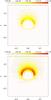 |
Fig. 5 Modeled image of the polarized flux, PF/F∗, for a centrally irradiated, optically thick torus with θ0 = 30° measured relative to the axis of symmetry; PF/F∗ is color–coded and integrated over the wavelength band. Top: face-on image at ~2175 Å; bottom: face-on image at ~7500 Å. |
The image in Fig. 4 (top) illustrates the discussion on the net polarization induced by scattering off of the inner surfaces of a dusty torus (see Kartje 1995, and Paper I): the surfaces parallel to the observer’s line of sight produce a polarization vector that tends toward an orientation of 90°, while the surfaces oriented perpendicularly to the line of sight produce a polarization vector at 0°. At an intermediate viewing angle (Fig. 4, bottom), the effects of extinction by dust become very strong. The inner wall opposite the observer is still visible but the walls on the side and the nearest inner surface disappear below the torus horizon. Often, the photons must undergo multiple scatterings inside the torus funnel before they escape and are observed. Because the absorption probability increases with the number of scattering events, we thus observe a lower polarized flux than at pole-on view. For a line of sight near the equator, no flux is observed owing to complete absorption by the optically thick dust. Therefore, we do not present the polarization map at an angle i of ~87°.
3.1.2. UV-to-optical polarization images
The net polarized flux coming from a given position on the torus inner walls is determined by a complex interplay between the dust albedo and the scattering phase function. Both of these properties are a function of wavelength. We therefore illustrate the wavelength-dependence of the polarization map in Fig. 5. The two maps are taken at the specific wavelengths of 2175 Å and 7500 Å, which correspond to a characteristic extinction feature in the UV and to a plateau region of the extinction cross-section in the optical. The spatial distribution in polarized flux differs significantly between the two wavebands, with the 7500 Å map showing a stronger PF/F∗. At 2175 Å, the scattering phase function greatly favors forward scattering over scattering to other directions. Since the torus is optically thick and its funnel is narrow, the photons are more likely to be absorbed. At 7500 Å, the scattering phase function is less anisotropic and therefore allows scattered (i.e., polarized) photons to escape more easily from the funnel. The fact that optical photons also encounter a slightly higher albedo in the dust grains than UV photons does work in the same direction. The combination of these effects explains why the spatial distribution in polarized flux in the optical reaches out to larger distances from the central source than in the UV waveband.
3.2. Modeling polar outflows
Polar outflows are a major constituent when explaining the AGN polarization behavior. They allowed the initial discovery of Seyfert-1 nuclei in Seyfert-2 objects by means of spectropolarimetry (Antonucci & Miller 1985). An approximative geometry of the polar scattering regions corresponds to an hourglass shape with a central break where the photon source is located. It is believed that below the dust sublimation radius the polar wind is mainly composed of ionized gas whereas beyond this radius, the gas can coexist with dust. We therefore modeled an electron-filled double-cone for the ionized material closer to the source as well as a pair of more distant, dusty outflows.
3.2.1. Modeling polar electron scattering
Using the formalism introduced by Brown & McLean (1977), Miller & Goodrich (1990) and Miller et al. (1991) were the first to compute the polarization from an AGN double-cone composed of electrons. Based on these results, Wolf & Henning (1999) and Watanabe et al. (2003) conducted Monte Carlo simulations that also include the effects of multiple scattering that were not taken into account in the analytical formula of Brown & McLean (1977). Paper I repeated and confirmed these studies. It turned out that a radial gradient of the electron density inside the double cone does not have a major impact on the resulting polarization. In most cases, a uniform density leads to very similar results. Here, we resume this investigation and add our new results for the polarization imaging.
We implemented the same polar wind characteristics as in Paper I and modeled a double cone filled with electrons. The electron density was adjusted to achieve a radial Thomson optical depth of τ ~ 1 measured in the vertical direction between the inner and outer surfaces of a single cone. The half-opening angle of the double cone is 30° measured from the vertical axis. Unlike the modeling in Paper I, we did not restrict the emission angle of the central source but considered isotropic emission.
The resulting polarization as a function of inclination is shown in Fig. 6. The polarization curve is very similar to the one found in Paper I (Sect. 5.1), but its normalization has drastically diminished. This is because of the strong dilution by the unpolarized radiation that comes directly from the source that we excluded in our previous modeling. Note that a second source of polarization dilution, not taken into account because we focused on the continuum emission, might also come from the recombination lines and continua. Such a radiative mechanism should then decrease the observed emission-line polarization and the Balmer continuum, e.g., and will be subject of our future work.
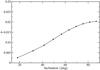 |
Fig. 6 Modeling an electron-filled, scattering double-cone with the half-opening angle θc = 30° measured relative to the symmetry axis. The net polarization, P, is plotted versus the observer’s inclination i. |
 |
Fig. 7 Modeled images of the PF/F∗ for an electron-filled, scattering double-cone composed of the half-opening angle θc = 30° measured relative to the symmetry axis. The polarized flux, PF/F∗, is color–coded and integrated over the wavelength band. Top: face-on image; middle: image at i ~ 45°; bottom: edge-on image. |
Polarization maps are given in Fig. 7. From a pole-on view, the highest PF/F∗ is concentrated below the (projected) center of the model space. It is dominated by photons back-scattered at the base of the far cone. Above the center, a secondary, dimmer maximum appears that originates from forward-scattering in the near cone. The slightly oval shape of the figure is a projection effect because the line of sight is inclined by 18° relative to the symmetry axis. The approximate symmetry at pole-on viewing position explains why the net polarization at this viewing angle is quite low. The distribution of polarization position angles across the image shows that the polarization produced on the left side of the line of sight partly cancels with that produced on the right side. The net γ in the pole-on view is oriented perpendicularly to the symmetry axis. Increasing i diminishes the spatial symmetry and thereby leads to a growth of the polarized flux. There is a flux gradient along the vertical axis. Photons that penetrate farther into the cone see a larger optical depth before escaping into an intermediate or edge-on viewing direction because of the conical geometry and uniform electron density. Multiple scattering therefore diminishes the resulting polarization produced farther away from the center.
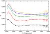 |
Fig. 8 Modeling a dusty double-cone of half-opening angle θc = 30° measured relative to the axis of symmetry. The spectrum of the polarization percentage P is plotted for different viewing inclinations, i. |
The strong radial gradient in polarized flux that we obtain in our modeling relates to the question of how strong the effect of a density gradient inside the double cone is on the net polarization (see Watanabe et al. 2003, and Paper I). Indeed, if the density gradient is steep near the source, the polarized flux produced at the base of the cones should diminish, but, at the same time, the polarization from the optically thinner outer parts of the cones rises because multiple-scattering becomes less important. It is thus not trivial to use polarimetry to constrain the radial density profile in conical scattering regions.
3.2.2. Polar dust scattering
Beyond the dust-sublimation radius of an AGN dust particles can survive or form. We therefore have to study the effect of dust absorption and scattering on the polarization induced by polar outflows. We used again the dust composition based on the Milky Way model (see Paper I and reference within) and defined a dusty double-cone with a half-opening angle equal to 30° from the vertical axis. The inner boundary of the scattering region was fixed at 10 pc above the source and the double cone extends to a distance of 100 pc. The optical depth in the V-band was fixed at τV ~ 0.3.
The polarization spectra are shown in Fig. 8. They are similar to the results of Paper I (except that the Poissonian fluctuations are smoother due to better statistics with the newly implemented MTG). We show the images of the polarized flux in Fig. 9. Unlike the case of the double cones of scattering electrons, the face-on view shows only one spatial maximum that corresponds to forward scattering in the near cone. The dust phase function favors forward scattering over backscattering, and therefore the far cone is dominated by absorption and cannot be seen in polarized flux. However, the same characteristics of the polarization position angle, γ, can be observed for both types of scattering media. At an intermediate viewing angle, we observe a higher polarized flux but still mainly dominated by the lower part of the upper cone. The behavior of the net polarization is again related to the spatial symmetry that changes with viewing angle, just as for the electron-scattering double cone described in Sect. 3.2.1. At an edge-on viewing position, mostly perpendicular polarization with a radial gradient is seen. Significant polarized flux still emerges close to the outer limits of the reprocessing region. For wavelengths above 2200 Å, the scattering cross section decreases monotonically so that photons can travel farther into the medium before they are scattered or absorbed.
3.2.3. The effects of the optical depth and wavelength
We studied the dependence of the polarization on wavelength and on the optical depth of the dusty outflows. We varied the optical depth of the medium in the V-band, τV, between 0.03, 0.3, and 3 and we show the imaging results in Figs. 10–12, respectively. Maps are shown for an edge-on viewing angle and at wavelengths of 2175 Å and 7500 Å.
 |
Fig. 9 Modeled images of the polarized flux, PF/F∗, for a dusty double-cone of half-opening angle θc = 30° measured relative to the axis of symmetry; PF/F∗ is color–coded and integrated over the wavelength band. Top: face-on image; middle: image at i ~ 45°; bottom: edge-on image. |
It appears from the color scale of the figures that up to a range of τV < 3 the PF/F∗ increases with τV. As the optical depth determines the average number of scattering events before escape or absorption, increasing it leads to more scattering and therefore to more PF/F∗, at least before the optical depth becomes sufficiently high depolarizing multiple-scattering effects to become predominant. The systematic rise in PF/F∗ seems to be similar at both wavelengths. Photons with longer wavelengths (i.e., ~7500 Å), pass through a larger portion of material before they are scattered and escape. This effect is related to the evolution of the extinction cross section with wavelength, as mentioned earlier.
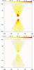 |
Fig. 10 Modeled images of the polarized flux, PF/F∗, for a dusty double-cone with the half-opening angle θc = 30° measured relative to the symmetry axis and a radial optical depth of τV ~ 0.03; PF/F∗ is color–coded and integrated over the wavelength band. Top: edge-on image at ~2175 Å; bottom: edge-on image at ~7500 Å. |
For our modeling of the dusty outflows the optical depth is always much lower (between 0.03 and 3) than the one assumed for the optically opaque torus (~750). The photons scattering off the outflows thus do not remain close to the surface of the scattering region but can penetrate deep into the medium before they are scattered or absorbed. At 2175 Å, the photon phase function favors forward- over backscattering. Photons that have already scattered and progressed in the direction of the observer are thus less likely to be scattered out of the line of sight. In general, the PF/F∗ is therefore greater at UV wavelengths than in the optical band.
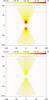 |
Fig. 11 Modeled images of the polarized flux, PF/F∗, for a dusty double-cone with the half-opening angle θc = 30° measured relative to the symmetry axis and a radial optical depth of τV ~ 0.3; PF/F∗ is color–coded and integrated over the wavelength band. Top: edge-on image at ~2175 Å; bottom: edge-on image at ~7500 Å. |
3.3. Equatorial scattering in a radiation-supported disk
To explain the presence of parallel polarization (with respect to the projected symmetry axis), a third type of scattering region has been proposed (Antonucci 1984): a radiation-supported, geometrically thin scattering disk that lies in the equatorial plane (Chandrasekhar 1960; Angel 1969; Sunyaev & Titarchuk 1985). Most often, the geometry of a flared wedge is assumed for this scattering region (see Fig. 17 in Paper I for a schematic review of the possible geometries). Following the suggestions of Goodrich & Miller (1994) and the simulations of Young (2000) and Smith et al. (2004, 2005), we showed in Paper I that the flared-disk geometry can be replaced by a torus geometry without noticeable changes in polarization. This substitution is consistent for a flared-disk half-opening angle lower than 30°. Here, we simulate an equatorial scattering region using a geometrically thin torus composed of electrons with a Thomson optical depth of τ ~ 1 and a half-opening angle of 10° with respect to the equatorial plane. The inner radius of the thin torus is 3 × 10⁻⁴ pc and its outer radius is 5 × 10⁻⁴ pc.
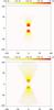 |
Fig. 12 Modeled images of the polarized flux, PF/F∗, for a dusty double-cone with the half-opening angle θc = 30° measured relative to the symmetry axis and a radial optical depth of τV ~ 3; PF/F∗ is color–coded and integrated over the wavelength band. Top: edge-on image at ~2175 Å; bottom: edge-on image at ~7500 Å. |
The polarization spectra as a function of the inclination i are shown in Fig. 13. A negative value of P indicates parallel polarization at all viewing angles. The spectra are very similar to those presented in Paper I for the geometry of a flared disk. Figure 14 presents the polarization maps for the simulated equatorial scattering disk. For a pole-on view, the disk is divided into concentric rings of polarized flux with polarization vectors oriented tangentially to the rings. By integrating the entire region, we obtain a polarization position angle of 90° for a nearly face-on viewing angle. The inner surface of the equatorial disk causes a lower polarized flux than the rest of the reprocessing region. The torus geometry implies that the inner region has a height (relative to the equatorial plane) that is less important than the central region. However, if the density is uniform throughout the medium; we deduce that the vertical column density is lower on the edges of the torus. Hence, the PF/F∗ is greater in the central part where the vertical column density and therefore the scattering probability is maximum. When we tilt the line of sight to an intermediate position, we observe a polarized flux greater on the torus surfaces which are parallel to the line of sight. These surfaces retain a strong polarization as long as the scattering angle with respect to the observer’s line of sight stays close to 90°. Surfaces orthogonal to the line of sight cause a lower PF/F∗ compared to the pole-on view. Therefore, the net polarization remains parallel and is even stronger at an intermediate view than at the near face-on view. For angles i at nearly edge-on view, the scattering geometry only allows for parallel polarization for all parts of the equatorial disk.
On the PF/F∗-plots the photon source seems hidden by the medium because it is seen only in transmission, which induces very low polarization. However, this strong, low-polarization flux dilutes more significant polarized flux coming from other areas of the scattering region. A second reason why the net polarized flux remains moderate is that at the optical depth τV = 1 considered here multiple scattering events occur inside the medium.
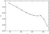 |
Fig. 13 Modeling of an equatorial, electron-filled scattering disk with a half-opening angle θ0 = 10° measured with respect to the equatorial plane. Polarization P is plotted against the inclination i along the axis of the observer. Negative values for P indicate a parallel polarization. |
4. Exploring the radiative coupling between two reprocessing regions
 |
Fig. 14 Modeled image of the polarized flux, PF/F∗, for an electron-filled, equatorial scattering disk with a half opening angle θ0 = 10° measured with respect to the equatorial plane; PF/F∗ is color–coded and integrated over the wavelength band. Top: face-on image; middle: image at i ~ 45°; bottom: edge-on image. |
After modeling the polarization induced by individual scattering regions, we now include the effects of radiative coupling between them. Especially for significant optical depths, the coupling turns out to be important and should be properly addressed by Monte Carlo methods (see the discussions in Goodrich & Miller 1994, and in Paper I). We apply a step-by-step method combining first only two scattering regions at a time. Then, we approach a more complete AGN model that is composed of three individual scattering regions (see Sect. 5). In the following we will not include the previously studied dusty outflows because the NLR regions responsible for dust signatures in polar scattering objects are situated farther away from the central engine than the three other reprocessing regions (Marin & Goosmann 2012).
All three models presented here feature the same unpolarized, isotropic central source that was described previously. The first model in this section consists of an equatorial, electron-filled disk and polar, electron-filled outflows (Sect. 4.1). The second model is composed of the equatorial disk and an optically thick, dusty torus (Sect. 4.2). The last model comprises an optically thick torus and polar outflows (Sect. 4.3).
4.1. Equatorial scattering disk and electron-filled outflows
The equatorial scattering disk was again simulated by a electron-filled, geometrically thin torus as described in Sect. 3.3. The polar electron-filled outflows were modeled according to Sect. 3.2.1. This model setup may be applicable to nonthermal AGN with very low toroidal absorption. This claim has been made for FR I radio galaxies (Chiaberge et al. 1999; Whysong & Antonucci 2004) and LINERs (Maoz et al. 2005).
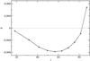 |
Fig. 15 Modeling electron-filled, polar outflows with a half-opening angle θc = 30° relative to the symmetry axis combined with an electron-filled, equatorial disk with a half-opening angle θ0 = 10° measured relative to the equatorial plane. The net polarization is plotted versus the inclination i of the observer. |
The resulting polarization percentage as a function of the viewing angle is shown in Fig. 15. At pole-on and intermediate viewing angles, P is negative (parallel net polarization). This is due to the predominance of the equatorial disk, which produces a polarization angle of γ = 90° regardless of the line of sight. At pole-on view, the parallel polarization that the photons acquire in the equatorial disk is preserved during their passage through the optically thin polar winds. Only toward the largest viewing angles the scattering polarization induced by the polar winds dominates and gives a net polarization angle of γ = 0°. P is always constant in wavelength because in this particular model we only considered Thomson scattering.
 |
Fig. 16 Modeled image of the polarized flux, PF/F∗, for the combination of an electron-filled, equatorial disk with electron-filled, polar outflows; the wavelength-independent PF/F∗ is color–coded and integrated over the complete wavelength range. Top: face-on image; middle: image at i ~ 45°; bottom: edge-on image. |
The polarization maps in Fig. 16 further illustrate our discussion. At pole-on view (Fig. 16, top), the double cone is visible in transmission and reflection. In many areas of the image, the polarization angle is at γ = 0°, however, the associated polarized flux remains weak compared to that coming from the equatorial disk, which has γ = 90°. The integrated PF/F∗ therefore has γ = 90°. The polarization images at intermediate viewing angles (Fig. 16, middle) partly agree with the results obtained for scattering in polar outflows alone (see Sect. 3.2.1). Again, the two maxima in polarized flux induced by scattering in the far and the near cone are visible and show perpendicular polarization. At the center, the impact of the equatorial disk is visible, and γ rotates toward 90°. Finally, when seen edge-on (Fig. 16, bottom), the net polarization has switched to γ = 0°. The scattered photons from the polar winds are now strongly polarized and dominate the net polarized flux.
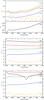 |
Fig. 17 Modeling an optically thick dusty torus with the half-opening angle θc = 30° relative to the symmetry axis combined with an electron-filled, equatorial disk with half-opening angle θ0 = 10° measured from the equatorial plane. Top: polarization, P, as seen at different viewing inclinations, i; middle: the fraction, F/F∗ of the central flux; bottom: the polarized flux PF/F∗. |
4.2. Radiation-supported disk and obscuring torus
Next, we considered a combination of the equatorial scattering disk with an optically thick, dusty torus. The parameterization of the reprocessing regions is the same as described before (see Sects. 3.3 and 3.1, respectively). The absence of polar outflows highlights a particular subclass of thermal Seyfert-1 AGNs that are characterized by a very weak or absent amount of intrinsic warm absorption (Patrick et al. 2011), a subclass also known as “bare” AGN.
Figure 17 shows, from top to bottom, the polarization percentage, the spectral flux, and the normalized polarized flux as a function of wavelength. At pole-on view, the behavior of P is particularly interesting: the polarization degree is negative in the UV-band, indicating parallel polarization. With increasing wavelength, the polarization weakens and undergoes a sign inversion around 5200 Å. For longer wavelengths, the polarization becomes again significant, but is perpendicular. This behavior is due to the competition in polarized flux between the equatorial disk and the torus. The two scattering regions produce polarization at opposite signs, but the albedo and scattering phase function of the dust change systematically with wavelength. Below 5200 Å, the phase function of Mie scattering strongly promotes forward scattering over scattering toward other directions. The dust albedo in the ultraviolet is slightly lower than at longer wavelengths so that, in total, bluer photons hitting the inner walls of the torus have a higher probability to be absorbed than redder photons. In the UV, the polarized flux emerging from the equatorial disk thus predominates. Above 5200 Å, the Mie scattering phase function is less anisotropic and the polarized flux scattered off of the torus inner walls and toward a pole-on observer becomes more important. The net polarization is then dominated by the torus and is perpendicular.
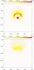 |
Fig. 18 Modeled image of the polarized flux, PF/F∗, for an electron-filled, equatorial disk combined with an optically thick, dusty torus; PF/F∗ is color–coded and integrated over the wavelength band. Top: face-on image; bottom: image at i ~ 45°. |
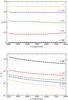 |
Fig. 19 Modeling an electron-filled double cone combined with an optically thick dusty torus, both with a half-opening angle of θc = 30° measured with respect to the symmetry axis. Results are shown for different viewing angles i. Top: polarization P; bottom: the fraction, F/F∗ of the central flux. |
At higher inclination, the equatorial scattering disk is hidden behind the torus and therefore its polarized flux with γ = 90° is not directly visible. The net polarization is now perpendicular across the whole waveband and rises toward longer wavelengths, as it does for the reprocessing of a dusty torus alone (see Fig. 3). The interplay between electron- and dust scattering is also visible in the F/F∗ spectrum (Fig. 17, middle). With increasing i, the spectral slope in the optical changes gradually. This behavior is again determined by the combined effect of the wavelength-dependent albedo and scattering phase function as well as by the specific scattering geometry chosen in this model. Comparison with the spectral flux obtained for a dusty torus alone (see Fig. 3) reveals that the negative slope for low viewing angles is an effect of the additional electron scattering that happens inside the torus funnel. The scattering feature of carbonaceous dust in the UV is seen only at intermediate and edge-on viewing angles. At pole-on view, the feature is blended by the direct flux from the source and by scattered radiation coming from the equatorial disk.
It is instructive to also discuss the polarized flux spectrum (Fig. 17, bottom) for this modeling case. At pole-on view, the PF/F∗ shows a minimum across the switch of the polarization position angle around 5200 Å and reduces the polarized flux by a large factor (note that when constructing the polarized flux we always take the absolute value of P). We should point out that the presence of the flip in polarization strongly depends on the exact model geometry and the scattering efficiency of the equatorial scattering disk. The strongest polarized flux occurs at a line of sight slightly below the torus horizon. Toward higher inclinations, the flux drops rapidly and so does PF/F∗.
The polarization maps are presented in Fig. 18. Due to the large difference in spatial scale between the two scattering regions, we restrict the mapping to the funnel of the dusty torus. At pole-on view (Fig. 18, top), the (wavelength-integrated) map shows that the polarized flux with γ = 0° coming from the dusty torus is almost of the same order of magnitude as the one emerging in the equatorial disk that carries γ = 90°. One has to take into account that the polarized flux spectrum reported in Fig. 17 is integrated over all scattering surfaces; with respect to the equatorial scattering disk, the polarized flux coming from a given position on the torus inner wall is lower, but this is compensated for by a larger integration surface. As discussed above, the exact outcome of the competition between the two components and the resulting polarization position angle depends on the wavelength. The situation is much clearer at an intermediate viewing angle (Fig. 18, bottom). Here, the polarized flux mostly emerges from the far-sided inner wall of the torus that induces γ = 0°. The near-sided wall and the walls on the side of the line of sight are barely visible because they are covered by the torus body. The equatorial scattering disk is hidden in the torus funnel so that the net polarization can only be equal to γ = 0°. We do not show the edge-on image for this model because almost all radiation is blocked by the optically thick torus.
4.3. Electron polar outflows and obscuring torus
Finally, we constructed a reprocessing model that combines the electron-filled polar outflows and the optically thick, dusty torus as presented previously in Sects. 3.2.1 and 3.1, respectively. This model setup would feature an AGN that (temporarily) lacks a material connection between the inner boundaries of the dusty torus and the outer parts of the accretion disk. The so-called “naked” AGN (Panessa & Bassani 2002; Hawkins 2004; Panessa et al. 2009; Tran et al. 2011) that seem to lack a BLR could fall into this category.
The spectropolarimetric modeling is presented in Fig. 19. The results reported in Sect. 3.1 show that at face-on viewing angles the polarization due to scattering off of a dusty torus is low and quite independent of wavelength. Here we obtained almost the same picture because the photons pass through the optically thin wind mostly by forward- or backward scattering. When the line of sight crosses the torus horizon, the dilution by the unpolarized source flux is suppressed and the polarization reaches higher values. With even higher inclination, there are two effects that increase the normalization of the polarization spectrum: firstly, there are more dust scattering events necessary to escape from the torus funnel. The systematic multiple scattering sharpens the perpendicular polarization. In many other situations multiple scattering is a depolarizing effect. The polarization sharpening established here is closely linked to the narrow funnel-geometry and the high optical depth of the torus, which makes only scattering off of its surface important. The second effect relates to the outflow in which stronger polarization is produced for higher i. This is due to the shape of the polarization phase function of Thomson scattering.
In contrast to the modeling of a torus alone (see Sect. 3.1), here the F/F∗ spectrum decreases toward longer wavelengths at all viewing angles considered; we discussed in Sect. 4.2 that additional electron scattering inside the torus funnel tends to decrease the spectral slope. In this respect, the polar outflows are even more efficient than the equatorial disk. The effect is again related to the change in scattering phase function from the UV to the optical waveband: the electrons inside the torus funnel scatter primary photons toward the torus inner surfaces. Since these surfaces have a receding shape toward the exit of the funnel, the scattered photons impinge it at a grazing angle. In the UV, the scattering phase function largely favors scattering into a cone of ~30° half-opening angle around the forward direction. This gives many photons a good chance to be scattered only once by the dust and then to escape from the torus funnel. Optical photons are more often scattered to a direction that leads back into the funnel and therefore they are slightly more likely to be absorbed. This explains why the scattered spectrum of the torus is stronger in the UV than in the optical waveband (even though the albedo in the UV is slightly lower than in the optical).
 |
Fig. 20 Modeling the polarized flux, PF/F∗, of electron-filled, polar outflow combined with an optically thick, dusty torus; PF/F∗ color–coded and integrated over all wavelengths. Top: face-on image; middle: image at i ~ 45°; bottom: edge-on image. |
As for the case of a scattering torus alone, the normalization of the F/F∗-spectrum decreases toward a higher viewing angle because the visible scattering surfaces of the funnel become rapidly smaller. Also, the scattering efficiency inside the polar outflows is lower for scattering toward higher i than toward a pole-on direction. At all type-2 inclinations, a dim feature of dust reprocessing in the UV is visible and traces the radiation component that is scattered into the line of sight by the torus.
The polarization maps are shown in Fig. 20. At pole-on view, the spatial maximum that is related to the far cone (seen in reflection) is less extended than the one related to the near cone (seen in transmission); compared to the pole-on image of an isolated, electron-filled outflow (see Sect. 3.2.1), the situation is reversed. This shows how the reflected flux from the far cone is partially blocked by the optically thick torus. Nevertheless, a significant polarized flux comes from the central region of the model, which is caused by the combined scattering inside the bases of the double cone and off of the inner torus walls, both producing perpendicular polarization. The two scattering regions thus reinforce each other in terms of polarization efficiency and the net polarization is, of course, perpendicular.
At an intermediate viewing angle, the double cone is more significantly hidden and the far cone is no longer visible at all. Much polarized flux still comes from the near cone, and compared to the isolated outflow, the gradient in PF/F∗ between the base and the outer regions is more shallow. This is related to the collimating effect of the torus funnel that efficiently channels photons (back) toward the outflow. Moreover, we point out the presence of a secondary scattering component coming from regions of the dusty torus that are not directly exposed to the source irradiation. When compared with the polarization map at intermediate view toward an isolated torus (see Sect. 3.1), this component becomes particularly visible on surfaces of the torus that are on the near side with respect to the line of sight. The photons that constitute this component have first undergone back-scattering inside the outflow and then were scattered off of the torus surface and toward the observer. This process is possible because the dusty torus has a significant average albedo of ~0.57 in the optical/UV band.
Finally, at edge-on view, the more distant areas of both the upper and the lower parts of the double cone are visible in reflection again. The center of the image shows no polarized flux due to the entirely opaque torus. The two extensions of the outflow scatter photons around the opaque torus and thereby produce strong polarization at a perpendicular orientation. Visualizing the polarized flux therefore enables us again to have a periscope view at the hidden nucleus.
5. Modeling the unified scheme of AGN
To approach the unified AGN scheme, we built a complex model composed of three radiatively coupled reprocessing regions: around the point-like, emitting source we arranged an equatorial electron scattering disk, polar electron outflows, and an obscuring dusty torus. The parameters of the model are summarized in Table 1. We investigated the polarization spectra and images for this particular model and then explored the parameter space in more detail by varying the geometry and optical depths of the equatorial and polar scattering regions.
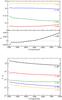 |
Fig. 21 Modeling the unified scheme of a thermal AGN by three reprocessing regions (see text). Top: polarization, P, as a function of viewing inclination, i; bottom: the fraction, F/F∗, of the central flux F∗. |
 |
Fig. 22 Modeling the polarized flux, PF/F∗, induced by complex reprocessing in a unified model of AGN. We combined an electron-filled, equatorial scattering disk, electron-filled polar outflows, and an optically thick dusty torus; PF/F∗ is color–coded and integrated over all wavelengths. Top: face-on image; middle: image at i ~ 45°; bottom: edge-on image. |
5.1. Spectral modeling results
The spectral results for the model described in Table 1 are shown in Fig. 21. At pole-on view, P is negative in the UV (parallel polarization) but of very low magnitude as the system appears to be almost axis-symmetric. Similarly to the polarization spectrum obtained for the combination of a dusty torus and an equatorial scattering disk, a sign inversion is detected between shorter and longer wavelengths. With respect to the results of Fig. 17 (top), the transition wavelength is shifted by the additional presence of the polar outflows. The exact wavelength at which the polarization angle switches also depends on the adopted outflow geometry and optical depths. At intermediate viewing angles, the effects of Mie scattering are visible by a weak feature in the UV band and a slight slope of the polarization spectrum over optical wavelengths. The F/F∗ spectrum also reveals the influence of wavelength-dependent dust scattering and absorption in the torus funnel by a gradually decreasing flux toward longer wavelengths, which is caused by the additional electron scattering inside the torus funnel (see the discussion in Sects. 4.2 and 4.3). A small peak of the flux around 2175 Å is caused by carbonaceous dust and visible at low and intermediate viewing angles. When i is increased even more the radiation becomes dominated by wavelength-independent, nearly perpendicular electron scattering inside the polar winds and P can achieve high values of more than 70%.
5.2. Wavelength-integrated polarization images
The polarization maps of our thermal AGN model are presented in Fig. 22. At pole-on view (Fig. 22, top), the distribution of the polarized flux is somewhat similar to the one obtained for the combination of an equatorial disk and a dusty torus only (Fig. 18, top); the effect of the polar outflows on the polarization at this viewing angle is quite small; with the strongest polarized flux coming from the equatorial scattering disk, the net polarization is parallel – as is observed in many type-1 AGN.
At intermediate viewing angles, the equatorial disk and the primary source are hidden by the optically thick torus. Nevertheless, the polarization produced at the base of the near cone (seen in reflection) is influenced by scattering inside the equatorial disk. The equatorial disk scatters a certain fraction of the primary radiation toward the outflows and induces parallel polarization. The perpendicular polarization caused by the secondary scattering inside the electron-filled double-cone is thus weakened when compared to the model that does not include the equatorial scattering disk (see Fig. 20, middle).
The base of the far cone is not visible because it is hidden behind the opaque torus. Instead we detect, as in the modeling presented in Fig. 20 (middle), a low polarized flux scattered off the near inner surfaces of the torus. The photons of this flux have been back-scattered from the polar winds onto the torus and then towards the observer. The overall polarization position angle at intermediate viewing angles is γ = 0°.
At edge-on view (Fig. 22, below), only the most upper and lower parts of the double cone appear above and below the body of the torus, which completely hides the central region of the model. The polarization effects caused by the equatorial disk are now largely exceeded by scattering in the outflows at almost perpendicular scattering angles. The resulting net polarization is therefore perpendicular and of high degree. Note that the adopted viewing angle in Fig. 22 is close but not exactly equal to 90°, which explains the asymmetry between the top and bottom part of the polar winds.
In Figs. 23 and 24 we show the pole-on and edge-on polarization map at two different wavelengths, 2175 Å (UV, top) and 7500 Å (optical, bottom), respectively. For all viewing directions a higher PF/F∗ is observed at 2175 Å, which is mainly caused by the larger spectral flux F/F∗ in the UV because the polarization is almost wavelength-independent (see Fig. 22). In Sects. 4.2 and 4.3, we have explained the importance of additional electron scattering inside the funnel for the resulting polarization. The polarization maps additionally illustrate the mechanism. At pole-on viewing angles, the polarized flux in the UV comes from a larger surface area around the torus funnel showing that photons that are scattered to these positions have a higher probability to escape toward the observer than in the optical. Some of these UV photons are then scattered again in the polar outflows and are redirected toward the observer, which is why the scattered UV-flux from the winds is more significant at an edge-on view.
Parameters for a thermal AGN model consisting of three scattering regions.
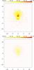 |
Fig. 23 Modeling the polarized flux, PF/F∗, of an AGN composed of an equatorial scattering disk, electron-filled, polar outflows and an optically thick dusty torus; PF/F∗ is color–coded and integrated over all wavelengths. Top: pole-on image at ~2175 Å; bottom: pole-on image at ~7500 Å. |
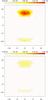 |
Fig. 24 Modeling the polarized flux, PF/F∗, of an AGN composed of an equatorial scattering disk, electron-filled, polar outflows and an optically thick dusty torus; PF/F∗ is color–coded and integrated over all wavelengths. Top: edge-on image at ~2175 Å; bottom: edge-on image at ~7500 Å. |
5.3. The impact of geometry and optical depth
Starting from our base-line model of a thermal AGN, we investigated how the spectropolarimetric results depend on several crucial model parameters. We computed a grid of models by varying the half-opening angle of the dusty torus and the polar winds as well as the optical depth of the electron scattering regions. We considered a common half-opening angle of the torus and the polar outflow and varied it between 30° and 60°, thereby implicitly assuming that the torus always collimates the outflow. The different optical depths assumed in the winds and the equatorial scattering regions can be interpreted as different mass transfer rates in both the accretion and the ejection flow.
A major motivation for our model grid is to explore the behavior of the polarization dichotomy between type-1 and type-2 thermal AGN. Bearing in mind the results obtained in Sect. 4, we chose a base-line model that optimizes the production of parallel polarization at type-1 lines of sight. This means in particular that we limited the spatial extension of the polar winds that produce only perpendicular polarization; in all modeling cases, the outer parts of the winds still reach out of the torus funnel but their contribution to the polarization at a type-2 viewing angle remains moderate. We also explored a broad range of optical depths for the wind reaching down to low values (0.03–1) and we excluded additional dusty, polar scattering regions located farther out. We studied a range of optical depths (0.1–5) and half-opening angles (10°, 20°, and 30°) for the equatorial scattering disk that covered its maximum efficiency to produce parallel polarization (see Paper I).
We present our results in Figs. 25–27 for the three half-opening angles of the equatorial scattering region, respectively. It turns out that the wavelength-dependence of P is fairly low therefore the absolute value of P is averaged in our grid. The geometry of the model strongly influences the polarization response: a narrow torus and skinny polar outflows (half-opening angle of 30° from the axis) produce strong perpendicular polarization, as was discussed in Kartje (1995) and Paper I. A wide opening angle of the object (half-opening angle of 60° from the axis) acts in the opposite way because it weakens the perpendicular polarization coming from the polar outflows and, at the same time, the wide torus produces parallel polarization and thereby reinforces the polarization signature of the equatorial scattering disk.
Indeed for a half-opening angle of 60°, parallel polarization is detected at nearly all type-1 lines of sight. Exceptions from this rule occur for an optically and geometrically thick equatorial disk. If the half-opening angle of the disk exceeds 30°, multiple scattering sets in; then, the mechanism that produces parallel polarization becomes less effective and may lead to a polar-scattered object (see the discussion in Smith et al. 2004) with a relatively low but perpendicular polarization at type-1 viewing angles. This behavior occurs in particular when the optical depth of the outflow exceeds 0.3 and/or the optical depth of the equatorial disk is higher than 3.
Polar-scattered AGN are very likely to exist also for lower torus half-opening angles (≤ 45° from the axis). They occur when the outflows become sufficiently optically thick (τ ~ 1) or when the equatorial scattering is too optically thin (τ ~ 0.3 and smaller). In all other cases, the usual polarization dichotomy is reproduced: the transition from a parallel to a perpendicular polarization angle happens when the observer’s line of sight toward the primary source crosses the torus horizon. This behavior is not much affected by the geometry of the equatorial scattering disk as long as its half-opening angle stays below 20° and the winds are not too optically thick. It turns out that the most efficient equatorial scattering geometry to induce parallel polarization in a complex type-1 AGN is obtained for a disk half-opening angle between 10° and 20°. The exact position of this optimum depends on Thomson optical depths for equatorial and polar scattering.
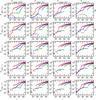 |
Fig. 25 Resulting percentage of polarization, P, as a function of viewing angle, i, for a complex AGN model (see text). The half-opening angle of the equatorial scattering disk is set to 10°. Legend: the different curves denote common half-opening angles of the torus and the polar winds of 30° (red squares), 45° (blue diamonds), and 60° (green triangles with points to the top). The isolated symbols indicate a polarization position angle γ = 90° (parallel), connected symbols stand for γ = 0° (perpendicular). From left to right: increasing the polar outflow optical depth from 0.03 to 1; From top to bottom: increasing the optical depth of the equatorial disk from 0.1 to 5. |
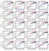 |
Fig. 26 Resulting percentage of polarization, P, as a function of viewing angle, i, for a complex thermal AGN model (see text). The half-opening angle of the equatorial scattering disk is set to 20°. The legend is as in Fig. 25. |
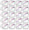 |
Fig. 27 Resulting percentage of polarization, P, as a function of viewing angle, i, for a complex thermal AGN model (see text). The half-opening angle of the equatorial scattering disk is set to 30°. The legend is as in Fig. 25. |
With increasing type-2 viewing angle, the percentage of the perpendicular polarization rises, which is related to a more favorable scattering angle for photons coming from the polar outflows. Apart from the scattering geometry, the behavior of the polarization dichotomy depends on the Thomson optical depths of both the polar outflow and of the equatorial scattering region. The observed polarization angle at a given line of sight results from a competition between the polarization efficiency of, on the one hand, the equatorial scattering region always producing parallel polarization and, on the other hand, the polar outflows that always imprint perpendicular polarization. Owing to its significant albedo of ~0.57, scattering off of the opaque torus has also an important impact, but here the position angle of the polarization depends on the torus opening angle.
The polarization percentage at type-2 viewing angles as a function of the outflow’s optical depth does not vary much, in particular for small or moderate opening angles of the object. The higher the Thomson optical depth of a medium, the more likely it is that an incident photon is scattered and polarized. Up to a certain limit the polarization induced by the medium accordingly rises, but if it becomes too dense, multiple scattering starts to depolarize the radiation. Hence, increasing the wind’s optical depth leads to a slightly higher P value until multiple scattering and depolarization set in and P decreases again. Investigating the impact of the flared disk’s optical depth, we find that optically thin disks (τ ≤ 0.1) are inefficient in producing parallel polarization at type-1 views. To produce parallel polarization, the optical depth of the disk should be higher than unity. The strongest parallel polarization is obtained for a scattering disk with 1 < τ < 3.
Our results show that the perpendicular polarization of optically thick winds (τ ~ 1) dominates over the parallel polarization coming from the equatorial disk except when the model has a large opening angle. For a more moderate and especially for a small opening angle, a net parallel polarization can be produced only when the outflows are sufficiently optically thin and, at the same time, the optical depth and the half-opening angle of the equatorial scattering region are in the right range. The interplay between polar and equatorial scattering may put constraints on the optical depth of the accretion flow if the optical depth and the geometry of the outflow in a given type-1 AGN can be estimated independently, for instance from the shape of UV and X-ray absorption lines. If it turns out that the effective optical depth in the outflow is above 0.3 and if at the same time the AGN reveals parallel polarization, we can conclude that a flattened accretion flow between the dusty torus and the accretion must be optically thick and in the range 1 < τ < 3.
6. Discussion
An important motivation of this work has been to investigate the net polarization caused by radiative coupling between the continuum source and different reprocessing regions of an AGN.
We considered electron scattering in an equatorial disk and in polar outflows as well as dust reprocessing by an obscuring torus. At first approach, it is reasonable to assume that the torus funnel collimates the polar outflows, which simplifies this multi-parameter problem. As a result, four parameters remain: the half-opening angles of the equatorial disk and of the torus/winds as well as the optical depths of the two electron scattering regions. The torus was always considered to be optically thick. Apparently the net polarization as a function of the viewing angle is most sensitive to the half-opening angle of the system and to a lesser extent on the geometry of the scattering disk, at least as long as it does not exceed a half-opening angle of 20° measured from the equatorial plane. A thicker equatorial disk favors multiple scattering and a partial disappearance of the parallel polarization. The optical depths of both electron scattering have a significant impact once they exceed ~0.3.
When compared to the observed optical/UV polarization, our systematic modeling can thus put constraints on certain AGN properties, as we discuss in more detail in the following.
6.1. Comparison with previous modeling work
There are several radiative transfer codes that include optical/UV polarization and that are applied in AGN research. Some of them only refer to continuum polarization (see e.g. Brown & McLean 1977; Manzini & di Serego Alighieri 1996; Kartje 1995; Wolf & Henning 1999; Watanabe et al. 2003) while others include details about the polarization of spectral lines (see e.g. Young 2000; Wang & Zhang 2007). Earlier works often applied semi-analytical or single-scattering methods. With greater computational power, Monte Carlo methods that include multiple scattering and more arbitrary geometries became suitable. In this section, we relate and compare our results to previous modeling work that is similar to ours.
To our knowledge, Wolf & Henning (1999) were the first and so far the only authors to simulate polarization images in the context of AGN. Their Monte Carlo code is based on earlier work by Fischer et al. (1994) which was also an important inspiration during the early development of stokes. In their application to AGN, Wolf & Henning (1999) included Mie scattering by two types of dust and electron scattering. Several reprocessing regions were investigated and gave rise to theoretical spectra and images of the intensity and polarization as a function of the viewing angle.
The AGN model adopted by Wolf & Henning (1999) is composed of (1) an obscuring dusty torus; (2) an electron-filled inner region and bi-conical outflow; and (3) an outer, dusty, bi-conical outflow. The authors showed that multiple scattering has an impact on the polarization as soon as the optical depths involved are higher than 0.1. A comparison to the geometry that we adopted in our work is not straightforward as there are differences in the details. For instance, the dusty torus employed by Wolf & Henning (1999) includes a cylindrical funnel. However, in our modeling we found a similar dependence of the polarization percentage on the viewing angle and also a good match in polarization images. We would like to point out that Wolf & Henning (1999) also investigated the effects of electron scattering inside the torus funnel. Their Fig. 13 shows that the resulting polarization spectrum becomes more concave for more centralized distributions of electrons. This agrees with our results and in Sects. 4.2 and 4.3 we gave an explanation of the effect based on the Mie scattering phase function and scattering geometry. Note that Kartje (1995) also considered the effects of additional electron scattering inside the torus but he did not vary the geometry of the electron distribution.
By also including a discussion on the net polarization angle as a function of viewing direction, we here extend the modeling performed by Wolf & Henning (1999), who did not discuss the polarization dichotomy. Producing parallel polarization for type-1 objects must be very hard in their adopted geometry as it lacks an equatorial scattering disk. Equatorial scattering, however, is included in the Generic Scattering Model (GSM) by Young (2000) and was subsequently applied by Smith et al. (2004) to explain strong, yet systematic variations of the polarization across broad emission lines. In addition to the interesting dynamical constraints that the model provided for the BLR, it also predicts a sequence in viewing angle for the continuum polarization. This sequence runs from type-1 AGN with parallel polarization to the so-called polar scattering dominated type-1 objects with perpendicular polarization (see Sect. 6.3.2) and ends at the type-2 AGN, again with perpendicular polarization.
The GSM analytically combines the polarized flux from the equatorial and polar scattering regions in a semi-analytical manner assuming single scattering. In Smith et al. (2004), the authors chose a Thomson optical depth of 0.2 for both electron scattering regions, a torus half-opening angle of 45° and an equatorial scattering disk with a half-opening angle of 20° or 30°. This configuration produced the strongest polarized flux with parallel polarization at type-1 viewing angles. Our Figs. 26 and 27 indicate that for a comparable case modeled with stokes, the resulting polarization at type-1 viewing angles is somewhat low compared to the observed range of generally ~0.3−1.3% (see Table Smith et al. 2002) or can even adopt a perpendicular polarization angle. One should take into account, however, that in our model we used a different geometrical shape for the equatorial scattering disk, a uniform density in all scattering regions, and we also considered the effects of multiple dust and electron scattering. Therefore, a comparison between both modeling schemes is not straightforward. We agree with Smith et al. (2004) in that a fairly flat equatorial scattering disk is required (half-opening angle < = 20°), but we prefer it to have a higher optical depth. Moreover, we found that systems with a torus half-opening angle significantly larger than 45° are better suited to produce the observed amount of parallel polarization in type-1 objects. We discuss the implications of our modeling on the polarization dichotomy in more detail in the following section.
6.2. Polarization at type-1 and type-2 viewing angles
In Sect. 5.3, we showed that for all modeling cases the polarization detected at a type-2 angle is strong and perpendicular. Even the most efficient equatorial scattering cannot force the net polarization to be parallel. If a thermal type-2 object with parallel polarization is observed, it cannot be explained by our current model and a possible re-interpretation then would be that the small-scale radio axis does not coincide with the symmetry axis of the dusty torus and/or the outflow.
The modeled perpendicular polarization at type-2 viewing angles covers a range of 30% to 80% for edge-on viewing angles. This would exclude the vast majority of Seyfert-2 galaxies that were analyzed by Kay (1994) and mostly showed polarization up to only 10%. Under the reasonable assumption that the distribution of viewing directions toward Seyfert galaxies is uniform, our modeling therefore suggests that the half-opening angle of most Seyfert-2 galaxies should be large, i.e., at least 60°. This conclusion would be consistent with the evolution model for Seyfert galaxies and the type-1/type-2 number counts given by Wang & Zhang (2007) but exceed those by Schmitt et al. (2001). On the other hand, it is not clear that the assumption of a universal half-opening angle for all dusty tori is realistic.
The situation is different for Seyfert-1 galaxies. The spectropolarimetric data collected by Smith et al. (2002) and Smith et al. (2004) show low polarization percentages mostly staying below 1%. However, it can have a parallel, perpendicular and sometimes also intermediate position angle. On the modeling side, the situation is equally ambiguous: narrow (i.e., geometrically thick) tori and outflows favor the production of perpendicular polarization for type-1 AGN while systems with wide (i.e., geometrically thin) tori and winds more likely produce type-1 AGN with parallel polarization, even when the outflows are optically thick. For the case of narrow tori, ionized outflows with an electron optical depth ranging from 0.03 to 1 still allows us to produce parallel net polarization at a type-1 viewing angle. Denser winds (τV ≥ 1) then switch the polarization to perpendicular. In any case, the resulting polarization percentage is low and therefore matches the observed values quite well.
However, it is noteworthy to point out that some peculiar type-1 AGN like Mrk 231 (Gallagher et al. 2005) and many Warm Infrared Ultraluminous AGN in the survey of Hines (1994) show a relatively high polarization degree, of up to 4%. Our grid of models is indeed unable to reproduce this high percentage of polarization despite the extended space of parameters. This indicates that the clue to this high polarization level must be different from the usual optical depth and half-opening angle considerations. In blazar AGNs, synchrotron emission can produce degrees of polarization superior to 30% in the UV/optical range while being strongly variable in time (Smith 1996). The amount of polarization is lower for extra-galactic, non-blazar, radio-loud objects, as in the case of OI 287 which exhibits P ~ 8% (Angel & Stockman 1980). In addition to the lack of polarization variability in time, Rudy & Schmidt (1988) and Goodrich & Miller (1988) proved with spectropolarimetric observations of OI 287 that the emission lines are polarized in a similar way to the continuum, ruling out a synchrotron origin. In addition to scattering, dichroic extinction might also increase the level linear polarization in face-on AGN if the dust grains are aligned by magnetic fields. Kartje (1995) showed that for not too optically thick (τV ≤ 10) dusty torii with partially aligned grains, the expected percentage of polarization might rise by 1.5%. Yet, in denser torii, scattering and dichroic extinction will partially cancel, causing P to increase more slowly. As our models present optically thick torii (τV = 750), dichroic extinction will not be sufficient to explain the high polarization percentages detected in Gallagher et al. (2005) or Hines (1994). A third explanation may come from IRAM PdBI observations of the extended outflows in Mrk 231 Cicone et al. (2012). They discovered a possible extension of the CO(1–0) transition blue wing a few arcseconds to the north, which remains unexplained. If we assume that the ionized polar outflows sustain the same half-opening angle and direction as the massive AGN-driven winds that can be considered as a naturally extended, dust mixed extension (Antonucci 1993; Cracco et al. 2011), the polar outflows in Mrk 231 might be nonaxisymmetric, similarly to NGC 1068 (Raban et al. 2009; Goosmann & Matt 2011). Because the system is seen from the pole, the overall picture would be less symmetric due to the winds inclination and then create an higher polarization degree. However, while the explanation of the high P detected in particular type-1 AGN might be an addition of the last three mechanisms proposed above, it is important to recognize that we have restricted the analysis in this paper to axially-symmetric situations while real AGNs are certainly messier and simple asymmetry could be the explanation. The significant long-term variability of the degree of polarization in Mrk 231 while the angle stays constant is qualitatively similar to what Gaskell et al. (2012) discussed for NGC 4151. As with NGC 4151, polarimetric reverberation mapping could give important information about the location of the main scattering region responsible for the relatively high polarization in Mrk 231.
The equatorial scattering region is important for determining the net polarization position angle for a type-1 view. If the half-opening angle of the system is intermediate or small (<45° from the axis), equatorial scattering with sufficient Thomson optical depth can still lead to parallel polarization at a type-1 viewing angle. The degeneracy between the impact of the torus/winds on the one hand and the equatorial scattering region on the other must be resolved by taking into account additional observables. We mentioned before that the analysis of UV and X-ray absorption lines in a type-1 AGN may constrain the optical depth in the outflow, but possibly the spectral slope of the polarization can also give a hint at the amount of equatorial scattering. When comparing the polarization spectra for a type-1 AGN in Figs. 17 and 21 to that in Fig. 19, it turns out that electron scattering inside the polar cones produces a flat polarization spectrum, whereas the equatorial scattering induces a concave shape in P. Comparing the broad-band continuum shape of the spectral flux to the polarization percentage can thus help to detect electron scattering that occurs deep inside the torus funnel.
In our modeling of AGN polarization we assumed very favorable conditions for the production of parallel polarization: the spatial extension of the ionization cones is relatively small and we did not consider additional dust scattering in farther away polar regions. Still, under these favorable conditions it turned out that the torus half opening should be quite large and the optical depth of the equatorial scattering region has to be about 1–3 to maximize the percentage of parallel polarization in type-1 views. Lower (τ < 0.3) optical depths will lead to the disappearance of parallel signatures and higher values (τ > 3) will decrease P through depolarization effects.
6.3. Constraining particular AGN classes
6.3.1. Bare and naked AGNs
The orientation unification model Antonucci (1993) explains the observed differences between type-1 and type-2 Seyfert galaxies as originating from orientation effects, but it is now recognized that orientation is not the whole explanation (Antonucci 2012). For example some Seyfert-1 AGN show weak or even no intrinsic warm absorption along the observer’s line-of-sight (Weaver et al. 1995; Patrick et al. 2011). These “bare” AGN allow a direct observation of the central engine.
Hawkins (2004) reported the presence of “naked” Seyfert-2 AGN, resulting from a survey of about 800 quasars and emission line galaxies. This new subclass is characterized by the weakness or even absence of the BLR and is coupled to strong optical variability, suggesting that the inner regions are not hidden anymore by an obscuring media. Those unabsorbed Seyfert-2 galaxies, which are part of a more general class called “nonhidden BLR” type-2 AGNs = NHBLR type-2s (Gliozzi et al. 2007), were mostly studied in the X-ray domain (Panessa et al. 2009; Gliozzi et al. 2010), i.e., without the help of spectropolarimetric tools.
For both of these subclasses of AGNs, spectropolarimetric measurements are not available and the absence of the cited reprocessing regions is based on X-ray analysis. In this paper, we presented a modeling case (see Sect. 4.3 for the naked model and Sect. 4.2 for the bare case) that can be compared to optical and UV observations. Such a broadband spectropolarimetric comparison can bring more information about the real nature of naked and bare AGNs as well as constrain the real morphology of these particular galaxies.
As is discussed at length in Antonucci (2012), it is often not clear whether the failure to detect a hidden BLR in polarized flux means that the AGN in a nonthermal AGN lacking a big blue bump and BLR or whether the failure is due the absence of a suitable scattering region to give us the needed periscopic view of the central regions. Polarization modeling can help us assess these two possibilities.
6.3.2. Polar-scattering-dominated AGN
A particular group of Seyfert-1 galaxies are known as polar-scattering-dominated AGN (Smith et al. 2002). In these type-1 objects the resulting polarization angle is perpendicular and relatively weak. In our reprocessing model, polar-scattering-dominated AGN generally have more strongly collimated outflows and tori with steep inner surfaces. Possibly, these objects also reveal a low polarized flux induced by (inefficient) equatorial scattering. However, if the polarization induced by equatorial scattering is strong, i.e., the equatorial scattering region is geometrically thin and has an optical depth of 1 < τ < 3, then the outflows must have a sufficiently column density to still produce a net polarization that is perpendicular.
Spectropolarimetric observations show that the optical polarization of polar-scattered AGN typically rises toward the blue. According to Smith et al. (2004), this wavelength-dependence is caused by dust extinction occurring along a line of sight that passes very close to the torus horizon, while still denoting a type-1 viewing angle. Material form the uppermost layers of the torus then produces a visible extinction of 1 < AV < 4 and causes the gradient in P. Our modeling shows this trend only for a torus half-opening angle of 45°. It leads to the very opposite spectral slope of P for more narrow tori. Thus, also the observed visible extinction in polar-scattering-dominated AGN indicates that the dusty torus should be rather wide than narrow. Note that for a torus half-opening angle of 60° no polar-scattering-dominated AGN exist in our model.
We will return to this problem in future work when we analyze in more detail the wavelength-dependence of our models also for clumpy media (see below), dust scattering in the polar regions, and different prescriptions for the dust. We have shown already that the polarization spectrum is quite sensitive to the dust composition and grain size distribution (Goosmann et al. 2007a,b).
6.4. More general geometries for the reprocessing regions
We have investigated the effects on our model results when one deviated from the adopted scales and geometry of certain scattering regions. This includes, in particular, the size of the obscuring torus and the geometrical shape of the equatorial scattering ring. Apparently a more compact torus with the same geometry and half-opening angle does not significantly alter the results. The same holds true when we replaced the toroidal scattering ring in the equatorial disk with a flared disk.
Our modeling assumed a uniform constant density across a given scattering region. This a considerable simplification. Observations of ionized outflows in AGN show that the winds should be at least partially fragmented. Using the spectropolarimetric capacities that were available on HST, Capetti et al. (1995) obtained spectropolarimetric and polarization imaging data of NGC 1068 in the UV. The authors detected a clumpy structure in polarization percentage and position angle. In most AGN, the ionized outflows cannot be spatially resolved and the polarized flux from a clumpy structure is integrated and only gives a net polarization for the entire outflow. By following this principle, Ogle et al. (2003) measured an average optical depth for the ionized outflows of NGC 1068 from spatially resolved X-ray observations with the HETGS onboard Chandra. The ratio of scattered X-ray continuum and emission line flux from the central region of the AGN gave an estimate of the Thomson optical depth of 0.27 ± 0.08. This confirmed the hypothesis that X-ray, NLR, and the optical/UV/X-ray reprocessing regions are likely to coincide.
There are more and more indications from observations and modeling in the IR that the obscuring torus should also have a clumpy structure (Nenkova et al. 2008b,a, 2010; Schartmann et al. 2008; Hönig & Kishimoto 2010; Heymann & Siebenmorgen 2012). For the future, a clumpy torus will be important to add to our modeling. We currently conduct preliminary studies for the expected optical/UV polarization of a centrally irradiated torus with a fragmented structure. So far, we find that, on the one hand, the normalization of the polarization spectra is significantly lower, while its spectral shape does not change much compared to the case of a uniform density torus. On the other hand, a clumpy torus allows more flux to escape from the central funnel, even at type-2 viewing angles that are strongly obscured by a uniform-density torus. Since the polarization efficiency is measured by the polarized flux emerging from the torus, we therefore expect that the torus remains an important scattering region even when it has a fragmented structure. Nonetheless, the lower polarization produced by a clumpy torus should lead to a weaker net polarization detected at type-2 viewing angles (see Sect. 5). This would help to bring our modeling results to better agreement with the observed spectropolarimetric data for Seyfert-2 galaxies (Kay 1994).
More general considerations about a clumpy but continuous accretion flow are currently discussed in the literature (see Elitzur 2007, and references therein for an overview) and therefore should be considered systematically in modeling work such as the one presented here. The clumpy nature of the dusty torus might also resolve the known problem that a geometrically thick torus lacks stability against self-gravity and therefore cannot be in hydrostatic equilibrium. The torus could rather be interpreted as a dynamical region of flowing, optically thick clouds. However, our modeling results and the observed parallel polarization in type-1 AGN as well as the moderate perpendicular polarization in type-2 objects argue against a geometrically thick torus (see Sect. 6.2).
Finally, we emphasize that in this work we always assumed the axes and half-opening angles of the dusty torus and the ionized outflows to be identical. A multi-wavelength analysis performed by Raban et al. (2009) suggests, however, that the bi-conical outflow in NGC 1068 should be inclined by ~18° with respect to the axis of the obscuring torus. The collimation effect on the ionized outflows might thus not be an obvious (although greatly simplifying) assumption in our modeling. We will investigate the consequences of this misalignment for the observed polarization spectra and images in a forthcoming paper (Marin et al., in prep.). This work is part of a multi-wavelength modeling attempt that also includes predictions for future X-ray polarimetry observations of NGC 1068 (Goosmann & Matt 2011). Some preparatory work on the optical/UV polarization signatures of the misaligned outflows in NGC 1068 at different azimuthal and polar viewing angles can be found in Marin et al. (2012a). It shows that the misalignment can lead to slightly higher parallel polarization in type-1 AGN and to systematically lower perpendicular P at a type-2 view. The latter effect would approach the model to the observational results by Kay (1994).
7. Summary and perspectives
We have upgraded the radiative transfer code stokes by implementing a more efficient random number generator and by adding the capability to model polarization imaging. The new version of the code is again made publicly available. We tested the new routines by reanalyzing the polarization signature of individual reprocessing regions, which then served as a basis for more sophisticated model setups.
We have combined three reprocessing components to analyze the complex radiative coupling occurring in Seyfert galaxies: (1) an ionized, equatorial scattering disk; (2) an optically and geometrically thick, dusty torus; and (3) an ionized, bi-conical outflow along the polar directions. We then computed the resulting polarization as a function of wavelength, projected position on the sky, and viewing angle. Our modeling shows that including multiple scattering effects inside a given scattering region and between several scattering regions is important.
As limiting cases, the model grid we presented also covers polarization caused by scattering in so-called bare and naked AGN.
In the general case of a unified model, it is possible to reproduce the observed dichotomy of the polarization angle for thermal AGNs within a limited range of geometries and optical depths:
-
1.
A flat, equatorial scattering region with 1 < τ < 3 is required to generate the observed parallel polarization in type-1 AGN. This indicates that the accretion flow at the outer edge of the accretion disk in Seyfert-1 galaxies is optically thick.
-
2.
A wide half-opening angle (~60°) for the torus helps to produce parallel polarization, whereas narrow tori and/or a higher optical depth of the polar outflow produce polar-scattering-dominated AGNs (the same AGNs show perpendicular polarization when seen at a type-1 viewing angle).
-
3.
At type-2 viewing angles, all cases we modeled produced perpendicular polarization that often is significantly stronger than the observed polarization percentage. Again, a wide half-opening angle of the torus and the wind help to lower this discrepancy with respect to the observations. It is likely, though, that a more significant moderation of the perpendicular polarization is caused by a clumpy structure.
-
4.
Detailed observations and modeling of the polarization spectrum may give hints on the presence of an equatorial electron scattering inside the torus funnel. We found that the equatorial scattering region leads to a more concave polarization spectrum than dust scattering off the inner torus walls alone. This type of modeling can help to explore the nature of AGNs that intrinsically seem to lack a BLR in more detail.
We explored in a preliminary and so-far purely theoretical manner the effects of multiple reprocessing in AGNs. In ongoing and future work we are also considering irregular reprocessing media and nonaxisymmetric setups. We will then proceed to compare our modeling to spectropolarimetric and imaging observations of individual objects.
“Naked” AGNs are a subclass of radio-quiet Seyfert 2 galaxies (so-called “nonhidden-BLR” Seyfert 2s = NHBLR Seyfert 2s) but show a less extended accretion regime than their parents. See Zhang & Wang (2006) for a parallel between NHBLR Seyfert 2s and Narrow Line Seyfert 1 AGN (NLS1), which both show high accretion rates.
In the literature on the possible role of AGN feedback on galaxy growth the two modes are sometimes referred to as “quasar mode” and “radio mode” but we prefer the labels “thermal” and “nonthermal” since historically the word “quasar” refers to a high-luminosity, radio-loud AGN. While all “quasars” are thermal AGNs, the converse is not true because the majority of thermal AGNs have a low luminosity.
There is an ongoing debate where there are NHBLR Seyfert 2s. Antonucci (2012) argued that we cannot conclude that NHBLR Seyfert 2s exist from existing evidence.
Acknowledgments
The authors would like to thank the anonymous referee for useful and constructive comments. This research has been supported by the French GdR PCHE, the mutual exchange program maintained by the French CNRS, the Academy of Sciences of the Czech Republic and the grant ANR-11-JS56-013-01. F.M. is grateful for financial and technical support from the Czech project COST-CZ LD12010. R.G. is grateful to the University of Valparíso for their hospitality. M.G. is grateful for support from the GEMINI-CONICYT Fund of Chile through project No 32070017 and FONDECYT No. 1120957. Finally, M.D. acknowledges support from the project RVO:67985815 and COST-CZ LD12010.
References
- Angel, J. R. P. 1969, ApJ, 158, 219 [NASA ADS] [CrossRef] [Google Scholar]
- Angel, J. R. P., & Stockman, H. S. 1980, ARA&A, 18, 321 [NASA ADS] [CrossRef] [Google Scholar]
- Antonucci, R. 1993, ARA&A, 31, 473 [Google Scholar]
- Antonucci, R. 2012, Astron., & Astrophys. Trans, in press [arXiv:1101.0837] [Google Scholar]
- Antonucci, R. R. J. 1982, Nature, 299, 605 [NASA ADS] [CrossRef] [Google Scholar]
- Antonucci, R. R. J. 1983, Nature, 303, 158 [NASA ADS] [CrossRef] [Google Scholar]
- Antonucci, R. R. J. 1984, ApJ, 281, 112 [NASA ADS] [CrossRef] [Google Scholar]
- Antonucci, R. R. J., & Miller, J. S. 1985, ApJ, 297, 621 [NASA ADS] [CrossRef] [Google Scholar]
- Bianchi, S., Corral, A., Panessa, F., et al. 2008, MNRAS, 385, 195 [NASA ADS] [CrossRef] [Google Scholar]
- Blandford, R. D., & Rees, M. J. 1978, Phys. Sci., 17, 265 [CrossRef] [Google Scholar]
- Brown, J. C., & McLean, I. S. 1977, A&A, 57, 141 [NASA ADS] [Google Scholar]
- Capetti, A., Macchetto, F., Axon, D. J., Sparks, W. B., & Boksenberg, A. 1995, ApJ, 452, L87 [NASA ADS] [CrossRef] [Google Scholar]
- Chandrasekhar, S. 1960, Radiative Transfer (New York: Dover) [Google Scholar]
- Chiaberge, M., Capetti, A., & Celotti, A. 1999, A&A, 349, 77 [NASA ADS] [Google Scholar]
- Cicone, C., Feruglio, C., Maiolino, R., et al. 2012, A&A, 543, A99 [NASA ADS] [CrossRef] [EDP Sciences] [Google Scholar]
- Costantini, E. 2010, Space Sci. Rev., 157, 265 [NASA ADS] [CrossRef] [Google Scholar]
- Cracco, V., Ciroi, S., di Mille, F., et al. 2011, MNRAS, 418, 2630 [NASA ADS] [CrossRef] [Google Scholar]
- Elitzur, M. 2007, in The Central Engine of Active Galactic Nuclei, eds. L. C. Ho, & J.-W. Wang, ASP Conf. Ser., 373, 415 [Google Scholar]
- Elvis, M. 2000, ApJ, 545, 63 [NASA ADS] [CrossRef] [Google Scholar]
- Elvis, M. 2004, in AGN Physics with the Sloan Digital Sky Survey, eds. G. T. Richards, & P. B. Hall, ASP Conf. Ser., 311, 109 [Google Scholar]
- Fischer, O., Henning, T., & Yorke, H. W. 1994, A&A, 284, 187 [NASA ADS] [Google Scholar]
- Gallagher, S. C., Schmidt, G. D., Smith, P. S., et al. 2005, ApJ, 633, 71 [NASA ADS] [CrossRef] [Google Scholar]
- Gaskell, C. M. 2008, in Rev. Mex. Astron. Astrofis. Conf. Ser., 32, 1 [Google Scholar]
- Gaskell, C. M. 2009, New A Rev., 53, 140 [Google Scholar]
- Gaskell, C. M., & Goosmann, R. W. 2008, ApJ, submitted [arXiv:0805.4258] [Google Scholar]
- Gaskell, C. M., Goosmann, R. W., Merkulova, N. I., Shakhovskoy, N. M., & Shoji, M. 2012, ApJ, 749, 148 [NASA ADS] [CrossRef] [Google Scholar]
- Georgantopoulos, I., & Zezas, A. 2003, ApJ, 594, 704 [NASA ADS] [CrossRef] [Google Scholar]
- Gliozzi, M., Sambruna, R. M., & Foschini, L. 2007, ApJ, 662, 878 [NASA ADS] [CrossRef] [Google Scholar]
- Gliozzi, M., Panessa, F., La Franca, F., et al. 2010, ApJ, 725, 2071 [NASA ADS] [CrossRef] [Google Scholar]
- Goodrich, R. W., & Miller, J. S. 1988, ApJ, 331, 332 [NASA ADS] [CrossRef] [Google Scholar]
- Goodrich, R. W., & Miller, J. S. 1994, ApJ, 434, 82 [NASA ADS] [CrossRef] [Google Scholar]
- Goosmann, R. W., & Matt, G. 2011, MNRAS, 415, 3119 [NASA ADS] [CrossRef] [Google Scholar]
- Goosmann, R. W. 2007, in Proceedings of RAGtime 8/9: Workshops on Black Holes and Neutron Stars, eds. S. Hledík, & Z. Stuchlík, 61 [Google Scholar]
- Goosmann, R. W., & Gaskell, C. M. 2007, A&A, 465, 129 [NASA ADS] [CrossRef] [EDP Sciences] [Google Scholar]
- Goosmann, R. W., Gaskell, C. M., & Shoji, M. 2007a, in IAU Symp. 238, eds. V. Karas, & G. Matt, 375 [Google Scholar]
- Goosmann, R. W., Gaskell, C. M., & Shoji, M. 2007b, in The Central Engine of Active Galactic Nuclei, eds. L. C. Ho, & J.-W. Wang, ASP Conf. Ser., 373, 485 [Google Scholar]
- Goosmann, R. W., Gaskell, C. M., & Shoji, M. 2008, in SF2A-2008: Proceedings of the Annual meeting of the French Society of Astronomy and Astrophysics, eds. C. Charbonnel, F. Combes, & R. Samadi, 231 [Google Scholar]
- Hawkins, M. R. S. 2004, A&A, 424, 519 [NASA ADS] [CrossRef] [EDP Sciences] [Google Scholar]
- Heymann, F., & Siebenmorgen, R. 2012, ApJ, 751, 27 [NASA ADS] [CrossRef] [Google Scholar]
- Hines, D. C. 1994, Ph.D. Thesis, Texas University [Google Scholar]
- Hönig, S. F., & Kishimoto, M. 2010, A&A, 523, A27 [NASA ADS] [CrossRef] [EDP Sciences] [Google Scholar]
- Kartje, J. F. 1995, ApJ, 452, 565 [NASA ADS] [CrossRef] [Google Scholar]
- Kay, L. E. 1994, ApJ, 430, 196 [NASA ADS] [CrossRef] [Google Scholar]
- Kazanas, D., Fukumura, K., Behar, E., Contopoulos, I., & Shrader, C. 2012, Astron. Rev., submitted [arXiv:1206.5022] [Google Scholar]
- Keel, W. C. 1980, AJ, 85, 198 [NASA ADS] [CrossRef] [Google Scholar]
- Knigge, C., Scaringi, S., Goad, M. R., & Cottis, C. E. 2008, MNRAS, 386, 1426 [NASA ADS] [CrossRef] [Google Scholar]
- Lawrence, A. 1991, MNRAS, 252, 586 [NASA ADS] [Google Scholar]
- Lodato, G. 2007, Nuovo Cimento Rivista Serie, 30, 293 [Google Scholar]
- Lynden-Bell, D. 1969, Nature, 223, 690 [NASA ADS] [CrossRef] [Google Scholar]
- Manzini, A., & di Serego Alighieri, S. 1996, A&A, 311, 79 [NASA ADS] [Google Scholar]
- Maoz, D., Nagar, N. M., Falcke, H., & Wilson, A. S. 2005, ApJ, 625, 699 [NASA ADS] [CrossRef] [Google Scholar]
- Marin, F., & Goosmann, R. W. 2011, in SF2A-2011: Proceedings of the Annual meeting of the French Society of Astronomy and Astrophysics, eds. G. Alecian, K. Belkacem, R. Samadi, & D. Valls-Gabaud, 597 [Google Scholar]
- Marin, F., & Goosmann, R. W. 2012, A&A, submitted [arXiv:1210.2899] [Google Scholar]
- Marin, F., Goosmann, R., & Dovčiak, M. 2012a, J. Phys. Conf. Ser., 372, 012065 [NASA ADS] [CrossRef] [Google Scholar]
- Marin, F., Goosmann, R. W., Dovčiak, M., et al. 2012b, MNRAS, 426, L101 [NASA ADS] [CrossRef] [Google Scholar]
- Marsaglia, G. 1985, IEEE Trans. Comp., 34, 756 [CrossRef] [Google Scholar]
- Mathur, S., Wilkes, B., Elvis, M., & Fiore, F. 1994, ApJ, 434, 493 [NASA ADS] [CrossRef] [Google Scholar]
- Mathur, S., Elvis, M., & Wilkes, B. 1995, ApJ, 452, 230 [NASA ADS] [CrossRef] [Google Scholar]
- Matsumoto, M., & Nishimura, T. 1998, ACM Trans. Model. Comput. Simul., 8, 3 [Google Scholar]
- Miller, J. S., & Goodrich, R. W. 1990, ApJ, 355, 456 [NASA ADS] [CrossRef] [Google Scholar]
- Miller, J. S., Goodrich, R. W., & Mathews, W. G. 1991, ApJ, 378, 47 [NASA ADS] [CrossRef] [Google Scholar]
- Nenkova, M., Sirocky, M. M., Nikutta, R., Ivezić, Ž. & Elitzur, M. 2008a, ApJ, 685, 160 [NASA ADS] [CrossRef] [Google Scholar]
- Nenkova, M., Sirocky, M. M., Ivezić, Ž. & Elitzur, M. 2008b, ApJ, 685, 147 [NASA ADS] [CrossRef] [Google Scholar]
- Nenkova, M., Sirocky, M. M., Nikutta, R., Ivezić, Ž., & Elitzur, M. 2010, ApJ, 723, 1827 [NASA ADS] [CrossRef] [Google Scholar]
- Ogle, P. M., Brookings, T., Canizares, C. R., Lee, J. C., & Marshall, H. L. 2003, A&A, 402, 849 [NASA ADS] [CrossRef] [EDP Sciences] [Google Scholar]
- Panessa, F., & Bassani, L. 2002, A&A, 394, 435 [NASA ADS] [CrossRef] [EDP Sciences] [Google Scholar]
- Panessa, F., Carrera, F. J., Bianchi, S., et al. 2009, MNRAS, 398, 1951 [NASA ADS] [CrossRef] [Google Scholar]
- Patrick, A. R., Reeves, J. N., Porquet, D., et al. 2011, MNRAS, 411, 2353 [NASA ADS] [CrossRef] [Google Scholar]
- Raban, D., Jaffe, W., Röttgering, H., Meisenheimer, K., & Tristram, K. R. W. 2009, MNRAS, 394, 1325 [NASA ADS] [CrossRef] [Google Scholar]
- Rudy, R. J., & Schmidt, G. D. 1988, ApJ, 331, 325 [NASA ADS] [CrossRef] [Google Scholar]
- Schartmann, M., Meisenheimer, K., Camenzind, M., et al. 2008, A&A, 482, 67 [NASA ADS] [CrossRef] [EDP Sciences] [Google Scholar]
- Schmitt, H. R., Antonucci, R. R. J., Ulvestad, J. S., et al. 2001, ApJ, 555, 663 [NASA ADS] [CrossRef] [Google Scholar]
- Smith, P. S. 1996, in Blazar Continuum Variability, eds. H. R. Miller, J. R. Webb, & J. C. Noble, ASP Conf. Ser., 110, 135 [Google Scholar]
- Smith, J. E., Young, S., Robinson, A., et al. 2002, MNRAS, 335, 773 [NASA ADS] [CrossRef] [Google Scholar]
- Smith, J. E., Robinson, A., Alexander, D. M., et al. 2004, MNRAS, 350, 140 [Google Scholar]
- Smith, J. E., Robinson, A., Young, S., Axon, D. J., & Corbett, E. A. 2005, MNRAS, 359, 846 [NASA ADS] [CrossRef] [Google Scholar]
- Sunyaev, R. A., & Titarchuk, L. G. 1985, A&A, 143, 374 [NASA ADS] [Google Scholar]
- Tran, H. D., Lyke, J. E., & Mader, J. A. 2011, ApJ, 726, L21 [NASA ADS] [CrossRef] [Google Scholar]
- Wang, J.-M., & Zhang, E.-P. 2007, ApJ, 660, 1072 [NASA ADS] [CrossRef] [Google Scholar]
- Watanabe, M., Nagata, T., Sato, S., Nakaya, H., & Hough, J. H. 2003, ApJ, 591, 714 [NASA ADS] [CrossRef] [Google Scholar]
- Weaver, K. A., Nousek, J., Yaqoob, T., Hayashida, K., & Murakami, S. 1995, ApJ, 451, 147 [NASA ADS] [CrossRef] [Google Scholar]
- Weymann, R. J., Morris, S. L., Foltz, C. B., & Hewett, P. C. 1991, ApJ, 373, 23 [NASA ADS] [CrossRef] [Google Scholar]
- Whysong, D., & Antonucci, R. 2004, ApJ, 602, 116 [NASA ADS] [CrossRef] [Google Scholar]
- Wolf, S., & Henning, T. 1999, A&A, 341, 675 [NASA ADS] [Google Scholar]
- Young, S. 2000, MNRAS, 312, 567 [NASA ADS] [CrossRef] [Google Scholar]
- Zhang, E.-P., & Wang, J.-M. 2006, ApJ, 653, 137 [NASA ADS] [CrossRef] [Google Scholar]
All Tables
All Figures
|
Fig. 1 Modeling a central, isotropic source that irradiates a dusty, equatorial scattering torus with a half-opening angle of 30° (see text). The spectrum represents the polarized flux, PF/F∗, normalized to the source flux F∗, for a viewing angle of i = 72°. The spectra were calculated by sampling the same number of photons but using two different random number generators. Black dashed line: the LCG algorithm as implemented in stokes 1.0; red solid line: the MTG algorithm as implemented in stokes 1.2. |
| In the text | |
|
Fig. 2 Spatial coordinates that determine the position of a photon P and its projection P′ onto the plane of the sky, D. |
| In the text | |
|
Fig. 3 Modeling an optically thick elliptically shaped torus with θ0 = 30° measured relative to the symmetry axis. The spatially integrated polarization P (upper panel) and the fraction F/F∗ of the central flux (lower panel) are seen at different viewing inclinations, i. |
| In the text | |
|
Fig. 4 Model image of the polarized flux, PF/F∗, for a centrally irradiated optically thick, elliptically shaped torus with θ0 = 30° measured relative to the symmetry axis; PF/F∗ is color–coded and integrated over the wavelength band. Top: face-on view at i ~ 18°; bottom: view at i ~ 45°. |
| In the text | |
|
Fig. 5 Modeled image of the polarized flux, PF/F∗, for a centrally irradiated, optically thick torus with θ0 = 30° measured relative to the axis of symmetry; PF/F∗ is color–coded and integrated over the wavelength band. Top: face-on image at ~2175 Å; bottom: face-on image at ~7500 Å. |
| In the text | |
|
Fig. 6 Modeling an electron-filled, scattering double-cone with the half-opening angle θc = 30° measured relative to the symmetry axis. The net polarization, P, is plotted versus the observer’s inclination i. |
| In the text | |
|
Fig. 7 Modeled images of the PF/F∗ for an electron-filled, scattering double-cone composed of the half-opening angle θc = 30° measured relative to the symmetry axis. The polarized flux, PF/F∗, is color–coded and integrated over the wavelength band. Top: face-on image; middle: image at i ~ 45°; bottom: edge-on image. |
| In the text | |
|
Fig. 8 Modeling a dusty double-cone of half-opening angle θc = 30° measured relative to the axis of symmetry. The spectrum of the polarization percentage P is plotted for different viewing inclinations, i. |
| In the text | |
|
Fig. 9 Modeled images of the polarized flux, PF/F∗, for a dusty double-cone of half-opening angle θc = 30° measured relative to the axis of symmetry; PF/F∗ is color–coded and integrated over the wavelength band. Top: face-on image; middle: image at i ~ 45°; bottom: edge-on image. |
| In the text | |
|
Fig. 10 Modeled images of the polarized flux, PF/F∗, for a dusty double-cone with the half-opening angle θc = 30° measured relative to the symmetry axis and a radial optical depth of τV ~ 0.03; PF/F∗ is color–coded and integrated over the wavelength band. Top: edge-on image at ~2175 Å; bottom: edge-on image at ~7500 Å. |
| In the text | |
|
Fig. 11 Modeled images of the polarized flux, PF/F∗, for a dusty double-cone with the half-opening angle θc = 30° measured relative to the symmetry axis and a radial optical depth of τV ~ 0.3; PF/F∗ is color–coded and integrated over the wavelength band. Top: edge-on image at ~2175 Å; bottom: edge-on image at ~7500 Å. |
| In the text | |
|
Fig. 12 Modeled images of the polarized flux, PF/F∗, for a dusty double-cone with the half-opening angle θc = 30° measured relative to the symmetry axis and a radial optical depth of τV ~ 3; PF/F∗ is color–coded and integrated over the wavelength band. Top: edge-on image at ~2175 Å; bottom: edge-on image at ~7500 Å. |
| In the text | |
|
Fig. 13 Modeling of an equatorial, electron-filled scattering disk with a half-opening angle θ0 = 10° measured with respect to the equatorial plane. Polarization P is plotted against the inclination i along the axis of the observer. Negative values for P indicate a parallel polarization. |
| In the text | |
|
Fig. 14 Modeled image of the polarized flux, PF/F∗, for an electron-filled, equatorial scattering disk with a half opening angle θ0 = 10° measured with respect to the equatorial plane; PF/F∗ is color–coded and integrated over the wavelength band. Top: face-on image; middle: image at i ~ 45°; bottom: edge-on image. |
| In the text | |
|
Fig. 15 Modeling electron-filled, polar outflows with a half-opening angle θc = 30° relative to the symmetry axis combined with an electron-filled, equatorial disk with a half-opening angle θ0 = 10° measured relative to the equatorial plane. The net polarization is plotted versus the inclination i of the observer. |
| In the text | |
|
Fig. 16 Modeled image of the polarized flux, PF/F∗, for the combination of an electron-filled, equatorial disk with electron-filled, polar outflows; the wavelength-independent PF/F∗ is color–coded and integrated over the complete wavelength range. Top: face-on image; middle: image at i ~ 45°; bottom: edge-on image. |
| In the text | |
|
Fig. 17 Modeling an optically thick dusty torus with the half-opening angle θc = 30° relative to the symmetry axis combined with an electron-filled, equatorial disk with half-opening angle θ0 = 10° measured from the equatorial plane. Top: polarization, P, as seen at different viewing inclinations, i; middle: the fraction, F/F∗ of the central flux; bottom: the polarized flux PF/F∗. |
| In the text | |
|
Fig. 18 Modeled image of the polarized flux, PF/F∗, for an electron-filled, equatorial disk combined with an optically thick, dusty torus; PF/F∗ is color–coded and integrated over the wavelength band. Top: face-on image; bottom: image at i ~ 45°. |
| In the text | |
|
Fig. 19 Modeling an electron-filled double cone combined with an optically thick dusty torus, both with a half-opening angle of θc = 30° measured with respect to the symmetry axis. Results are shown for different viewing angles i. Top: polarization P; bottom: the fraction, F/F∗ of the central flux. |
| In the text | |
|
Fig. 20 Modeling the polarized flux, PF/F∗, of electron-filled, polar outflow combined with an optically thick, dusty torus; PF/F∗ color–coded and integrated over all wavelengths. Top: face-on image; middle: image at i ~ 45°; bottom: edge-on image. |
| In the text | |
|
Fig. 21 Modeling the unified scheme of a thermal AGN by three reprocessing regions (see text). Top: polarization, P, as a function of viewing inclination, i; bottom: the fraction, F/F∗, of the central flux F∗. |
| In the text | |
|
Fig. 22 Modeling the polarized flux, PF/F∗, induced by complex reprocessing in a unified model of AGN. We combined an electron-filled, equatorial scattering disk, electron-filled polar outflows, and an optically thick dusty torus; PF/F∗ is color–coded and integrated over all wavelengths. Top: face-on image; middle: image at i ~ 45°; bottom: edge-on image. |
| In the text | |
|
Fig. 23 Modeling the polarized flux, PF/F∗, of an AGN composed of an equatorial scattering disk, electron-filled, polar outflows and an optically thick dusty torus; PF/F∗ is color–coded and integrated over all wavelengths. Top: pole-on image at ~2175 Å; bottom: pole-on image at ~7500 Å. |
| In the text | |
|
Fig. 24 Modeling the polarized flux, PF/F∗, of an AGN composed of an equatorial scattering disk, electron-filled, polar outflows and an optically thick dusty torus; PF/F∗ is color–coded and integrated over all wavelengths. Top: edge-on image at ~2175 Å; bottom: edge-on image at ~7500 Å. |
| In the text | |
|
Fig. 25 Resulting percentage of polarization, P, as a function of viewing angle, i, for a complex AGN model (see text). The half-opening angle of the equatorial scattering disk is set to 10°. Legend: the different curves denote common half-opening angles of the torus and the polar winds of 30° (red squares), 45° (blue diamonds), and 60° (green triangles with points to the top). The isolated symbols indicate a polarization position angle γ = 90° (parallel), connected symbols stand for γ = 0° (perpendicular). From left to right: increasing the polar outflow optical depth from 0.03 to 1; From top to bottom: increasing the optical depth of the equatorial disk from 0.1 to 5. |
| In the text | |
|
Fig. 26 Resulting percentage of polarization, P, as a function of viewing angle, i, for a complex thermal AGN model (see text). The half-opening angle of the equatorial scattering disk is set to 20°. The legend is as in Fig. 25. |
| In the text | |
|
Fig. 27 Resulting percentage of polarization, P, as a function of viewing angle, i, for a complex thermal AGN model (see text). The half-opening angle of the equatorial scattering disk is set to 30°. The legend is as in Fig. 25. |
| In the text | |
Current usage metrics show cumulative count of Article Views (full-text article views including HTML views, PDF and ePub downloads, according to the available data) and Abstracts Views on Vision4Press platform.
Data correspond to usage on the plateform after 2015. The current usage metrics is available 48-96 hours after online publication and is updated daily on week days.
Initial download of the metrics may take a while.