| Issue |
A&A
Volume 547, November 2012
|
|
|---|---|---|
| Article Number | A62 | |
| Number of page(s) | 31 | |
| Section | Catalogs and data | |
| DOI | https://doi.org/10.1051/0004-6361/201219804 | |
| Published online | 29 October 2012 | |
A catalogue of Paschen-line profiles in standard stars⋆
1
Department of AstronomyUniversity of Washington,
Box 351580
Seattle,
WA,
98195-1580,
USA
e-mail: wall@astro.washington.edu
2
Visiting Astronomer, Dominion Astrophysical Observatory, Herzberg
Institute for Astrophysics, Victoria, B.C.,
Canada
Received: 12 June 2012
Accepted: 27 August 2012
We have assembled an atlas of line profiles of the Paschen Delta (Pδ) line at 10 049 Å for the use of stellar modelling. For a few stars we have substituted the Paschen Gamma (Pγ) line at 10 938 Å because the Pδ line blends with other features. Most of the targets are standard stars of spectral types from B to M. A few metal-poor stars have been included. For many of the stars we have also observed the Hydrogen Alpha (Hα) line so as to compare the profiles of lines originating from the meta-stable n = 2 level with lines originating from the n = 3 level. The greatest difference in line profile is found for high luminosity and cool stars where the departures from local thermodynamic equilibrium (LTE) in the population of the n = 2 level is expected to be the greatest. For a few stars, sample line profiles have been calculated in the LTE approximation to demonstrate the usefulness of the tabulated and displayed catalogue.
Key words: line: profiles / atlases / stars: early-type / stars: late-type
The reduced observed spectra are only available at the CDS via anonymous ftp to cdsarc.u-strasbg.fr (130.79.128.5) or via http://cdsarc.u-strasbg.fr/viz-bin/qcat?J/A+A/547/A62
© ESO, 2012
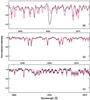 |
Fig. 1 Profiles for Hα, Pδ, and Pγ (a), b) and c) respectively) in HD 39801 (αOri) M2 Iab. The black line is the observed spectrum and the red line is the model spectrum. |
1. Introduction
The theory of model stellar atmospheres dates from the plane-parallel, single-layer models of Schuster (1902, 1905) and Schwarzschild (1906). In 1939 two very important papers on stellar atmospheres were published by Spitzer and by Struve, Wurm, and Henyey. In Spitzer’s (1939) paper on the atmospheres of M supergiants he noted that an excitation temperature of 17 000 K was necessary to explain the strength of the Hα absorption line in αOri even though the effective temperature of the star was about 3400 K. In Fig. 1, we show our recent spectrum of αOri with a resolving power of about 30 000. The observed Hα line (Fig. 1a) is prominent and does not appear in the spectrum as modelled with a standard atmosphere in local thermodynamic equilibrium (LTE). αOri’s Pδ line (Fig. 1b) is dominated by a blend of neutral lines, and its Pγ line (Fig. 1c) is obscured by a molecular band. Struve et al. (1939) called attention to the important fact that the 2s level from which the Balmer lines arise is meta-stable with a very small probability for the 2s → 1s transition. This may result in an over-population of the 2s level as compared with what is expected by the Boltzmann distribution in LTE. We quote them as follows, “It is tempting to explain the great strength of the Balmer absorption lines in supergiants of late type as a consequence of the metastability of the 2s level. However, it is premature to discuss this matter further until accurate measurements of the Paschen lines have been made”.
Most early work on stellar atmospheres was based on the assumption of LTE in which the relative populations of the atomic levels are controlled by the local temperature and the assumption that the radiation field is also dependent on the local temperature (Unsöld & Weidemann 1955). In succeeding years the degree of realism of model atmospheres has steadily increased, first, with sophistically calculated gradients of various physical quantities (Mihalas & Athay 1973), through models with extended atmospheres, to the most recent models with surface fluctuations of all relevant quantities. The most recent models include surface variations associated with large scale convection and granulation as well as departures from LTE in their excitation and ionization equilibria (Asplund 2005).
As noted by Struve et al. (1939), in real stars there is a special problem with the assumption of LTE because the radiative transition from the 2s level of hydrogen to the 1s ground state is forbidden. This means that the population of the 2s level must be controlled by radiative and collisional transitions with other excited levels, but transitions between the 2s and 1s levels are strongly inhibited. At high densities collisions are effective so that the population ratios among the n > 2 levels approach equilibrium but the relative populations between n = 1 and n = 2 deviate from LTE. The populations of all levels are influenced by recombination and ionization, especially in the hotter stars. There is no question as to the presence of non-LTE (NLTE) effects; the only question is one of degree. The Paschen lines which originate from the n = 3 level are expected to be closer to LTE than are the Balmer lines. To investigate the importance of these effects it is helpful to observe the Paschen (and higher) lines and to compare their line profiles with the predictions of atmospheric models. An additional consideration is the increased Stark effect for the Paschen lines as compared to the Balmer lines because Stark broadening increases with higher quantum numbers. Hence, the Stark broadening for the Paschen lines is expected to dominate over other broadening mechanisms.
Standard stars observed.
2. Observations
With these factors in mind we have been observing a wide variety of stars at both Hα and 10 049 Å Pδ. The data have been obtained almost entirely with the Coudé spectrograph of the 1.2-m telescope at the Dominion Astrophysical Observatory (DAO) of the Hertzberg Institute of Astrophysics at Victoria British Columbia. Their 1.2-m telescope with a single order Coudé spectrograph is the ideal instrument for a spectroscopic survey of bright stars in a limited wavelength region since it does not suffer from the rapidly varying continuum in each short order of an echelle system. The 96-inch camera provides a resolving power of about 30 000 over 250 Å at each setting of the first order of the grating. The detector is a SITE 4 CCD with 24 micron pixels. There is a low level of fringing in the near infrared that can be removed by flat-fielding to a remaining noise level of about 1%. Since the stars are bright, the remaining source of noise is proportional to the square-root of the number of electrons per pixel and to absorption by the earth’s atmosphere. The latter can be largely eliminated by division of a rapidly rotating bright hot star, though caution must be used since almost all such stars have their own hydrogen lines. For broad lines whose H-line profiles are defined by many pixels the noise level is unimportant. Wavelength calibration in the near infrared can be difficult due to the paucity of emission lines in most comparison arcs. This was readily overcome by observing the ThAr spectrum in the second order and simply multipying the wavelengths so calibrated by exactly 2.
For a few stars of types K and M there is an FeI line that blends with Pδ and the latter is quite weak. Since these stars are very bright in the near IR it was possible to observe the brighter ones with the SITE 4 at the Pγ line at 10 938 Å. The 10 830 Å line of HeI is present in some of those spectra.
To overcome the problem of the FeI blend with the 10 049 Å line in the cooler stars we included some metal-poor stars. Most of those stars are too faint for the 1.2-m telescope so they were also observed with the Apache Point Observatory 3.5-m echelle. In Table 1 we list the stars for which useful spectra were obtained at the DAO. We list the metal-poor stars observed at the Apache Point Observatory in Table 2. In both tables the columns are self-explanatory. The Mv values are derived from the parallaxes measured by Hipparcos (van Leeuwen 2007) if the measured parallax is at least 3 times its quoted probable error. Actually, most of the parallaxes are at least 5 times their quoted error. An asterisk is shown for stars whose parallax lies between 3.0 and 5.0 times its uncertainty. No Mv value is shown for stars with parallaxes of greater uncertainty.
3. The line profiles
The primary purpose of this paper is to make available accurate line profiles of selected Paschen lines so they may be used in connection with modelling stellar atmospheres. In addition, the Paschen lines may be used for calibrating the temperature scale and analysing the chemical composition of stellar atmospheres where minimizing the influence of NLTE is helpful. In a series of tables we present the line profiles as observed. Most of the stars are represented by the Pδ line at 10 049 Å. In a few stars, especially stars of type K and M, the FeI line blends with Pδ. As mentioned above, we have observed the Pγ line at 10 938 Å whenever possible in addition to including the metal-poor stars with weakened FeI lines. For many of the stars we also obtained Hα profiles which we show for comparison with the Paschen line profiles. In Table 3 we list the wavelength, excitation of the lower level, and the transition probability of the three lines in this study. Our complete digital spectra have been deposited with the Centre de Données astronomiques de Strasbourg for access to all astronomers. To provide a complete atlas of our observations we have included all of our line profiles as figures, and we illustrate a variety of line profiles for a wide range of spectral types.
4. LTE profile comparisons
We also carried out calculations of Hα and Pδ profiles for some stars using the Kurucz models in LTE (Kurucz 1993; Sbordone et al. 2004; Sbordone 2005), the ATLAS atmospheric model production code, and the SYNTHE spectral synthesis code (Kurucz 1993; Sbordone et al. 2004). The Stark broadened profiles in the SYNTHE code are “based on the quasi-static Griem theory with parameters adjusted in such a way that profiles from the Griem theory fit the (Vidal et al. 1973) profiles of the first members of the Lyman and Balmer series” (Cowley & Castelli 2002). Stellar parameters for profile modelling (see Table 4) were obtained from references in the online astronomical database SIMBAD with favorable weight given to the data of Fulbright (2000). Further details about the tools for atmosphere model preparation and line synthesis can be found online at the ATLAS, WIDTH and SYNTHE GNU Linux port1Home page and under the Download page.
The figures show the synthetic LTE profiles plotted in red and the observed spectra in black.
4.1. Comments on selected stars
4.1.1. Spectral sequence at high luminosity with LTE profiles
Atomic data for hydrogen lines.
HD 37128, B0 Iab: Hα (Fig. 2a) shows a typical P Cygni profile while Pδ (Fig. 2g) is symmetric.
HD 46300 (13 Mon) A0 Ib: For 13 Mon there is a small difference in the profile of Hα (Fig. 2b) while the Paschen line (Fig. 2h) fits the model almost exactly.
HD 182835, F2 Iab: As for HD 46300, there is a small difference between the model and the observations in the line wings (Fig. 2c). The Paschen line fits almost exactly (Fig. 2i).
HD 209750, G2 Ib: The observed Hα line (Fig. 2d) appears to be wider than the model, while the model and observation of the Pδ line (Fig. 2j) fit very well.
HD 206778, K2 Ib & HD 42543, M0 Iab: The trend as the spectral type becomes later shows the observed Hα line (Figs. 2e, f) becoming steadily stronger as compared to the model.
Model hydrogen line profile parameters.
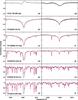 |
Fig. 2 Profiles of Hαa)–f) and Pδg)–l) for selected stars of high luminosity. |
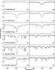 |
Fig. 3 Profiles of Hαa)–f) and Pδg)–l) for selected stars of high luminosity. |
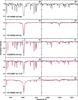 |
Fig. 4 Profiles of Hαa)–e) and Pδg)–k) for selected spectral type K stars. |
4.1.2. Sequence at high luminosity at mid-spectral types
HD 34085 (Rigel) B8 Iab: This standard B supergiant shows a self-absorbed Hα emission line (Fig. 3a) and a symmetric Pδ line (Fig. 3g).
HD 17378, A5 Ia: This supergiant member of the h and χ Per association is a little cooler than αCyg and shows an almost symmetric Hα line (Fig. 3b) at the time of observation with little evidence for either a wind or active chromosphere.
HD 20902 (αPer) F5 Iab: The fit for Hα (Fig. 3c) is very good and for Pδ (Fig. 3i) is almost perfect.
HD 77912, G8 Ib-II: The strong absorption at Hα (Fig. 3d) contrasts with the weaker line at Pδ (Fig. 3j).
HD 44537, K5 Iab: The Hα line (Fig. 3e) is strongly present and asymmetric. The Pδ line (Fig. 3k) is dominated by a blend of neutral lines.
HD 156014, M5 Ib-II: Despite the late spectral type, the observed Hα profile (Fig. 3f) remains strong.
4.1.3. Spectral type K stars
HD 122563, K0 IIp: This very metal-poor giant, whose [Fe/H] = −2.7, shows only small deviations from the model for its Hα (Fig. 4b) and Pδ (Fig. 4h) lines.
HD 232078, K3 IIp: (Figs. 4c and 4i) This red giant is in a markedly retrograde orbit and is similar to globular cluster red giants. Its Teff of 4000 K is one of the lowest values for a metal-poor field star. With [Fe/H] = −1.6, the metallic lines still obscure the Pδ line.
HD 124897 (Arcturus) K1.5 III: For this moderately metal-poor star, the observed Hα line (Fig. 4d) is much stronger than the model profile but the Pδ line (Fig. 4j) fits the model very well.
HD 103095 (Groombridge 1830) K0 Vp: This well-known, metal-poor main sequence star, with a Teff of 5000 K, appears to have a slightly deeper core at Hα (Fig. 4e) and shallower core at Pδ (Fig. 4k) than predicted.
4.1.4. Pγ profiles
HD 172167 (Vega) A0 V: This fundamental standard for modelling stellar atmospheres shows a very good fit between the modelled and the observed profile for Pγ (Fig. 5a).
HD 31964, A8 Iab: The Pγ line is clearly shown (Fig. 5b).
HD 20902 (αPer) F5 Iab: There is a great deal of blending at 10 938 Å, but the Pγ line is visible (Fig. 5c).
HD 206778, K1.5 III: The Pγ line is obscured by a molecular band (Fig. 5d).
4.2. Additional comments on selected stars
Figure 15, HD 886, B2 IV: This standard early B star shows symmetrical Hα and Pδ profiles.
Figure 41, HD 197345 (Deneb) A2 Iae: This standard supergiant shows its well-known P Cygni structure at Hα while its Pδ profile fits the model exactly.
Figure 52, HD 18391, G0 Ia: This G supergiant may be an outer member of the h and χ Per cluster. Its H lines appear to be symmetric.
Figure 69, HD 6860, M0 III: The Hα line is clearly present while the Pδ line is dominated by the blend of neutral metals. There appears to be almost no feature at Pγ. A weak molecular band may be interfering.
Figure 71, HD 206936 (μCep) M2 Ia: This supergiant may be even more luminous than αOri. Its Hα line is similar to that of αOri. There is no evidence for the Pγ line though the molecular band seen in αOri is weaker in μCep.
Figure 79, HD 172380 (XY Lyr) M4 Iab: Hα is clearly present while Pγ is not evident. The molecular band seen in αOri is not present.
Figure 80, HD 197812 (U Del) M5 Ia: A weak molecular band appears in the star and in most stars of type M5 or later very close to the position of Hα. No line is visible at Pγ.
Figure 85, HD 221170, G2 IV: Hα is symmetrical and much stronger than Pδ.
Figure 94, HD 25329, K1 V: This subdwarf is significantly metal-poor and is similar to HD 103095. For both stars Hα is much stronger than Pδ.
Figure 95, HD 165195, K3 p: This star’s metallicity is similar to giant branch stars in globular clusters and shows weak Hα emission that is usually associated with mass loss.
5. Discussion
Because the NLTE effects are much reduced in main-sequence stars, we expect that the synthesized LTE profiles should fit well with both Hα and Pδ observation. The result in Fig. 6 (for Vega, A0 V) is a very good example of this case, the LTE model (Teff = 9540 K, logg = 4.0) fit both Hα and Pδ well. But for the A0 supergiant, 13 Mon (HD 46300, A0 Ib), an LTE model can not match them simultaneously. When the LTE model matches the observed Pδ well (see Fig. 2h), it overestimates the strength of Hα (see Fig. 2b).
For super giants with lower temperature (but hotter than F5), we continue to see a similar difference between Hα and Pδ fittings which, however, become smaller towards lower temperatures (see Figs. 2c and 2i). The difference disappears around the spectral type of F5 (αPer, F5 Iab, in Figs. 3c and 3i, for example).
When the effective temperature drops to that of G type, the LTE models once again show their failure to reproduce the observed Hα profiles. In contrast to the case of hot luminous stars (Figs. 6, 2b, 2h), this time the LTE model profiles of Hα are weaker than the observed line profiles (Fig. 2d).
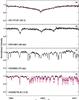 |
Fig. 5 Profiles of Pγ for select stars. |
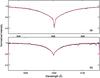 |
Fig. 6 HD 172167 (Vega) A0 V: except for a very small deviation at the center of the Hα profile, this fundamental standard for modelling stellar atmospheres shows a very good fit between the modelled and the observed profiles for Hα and Pδ. |
In the low temperature regime of K and M type giants/supergiants, the Hα profiles predicted by the LTE models become very weak while the observed profiles maintain their strength to appear almost the same as this of G stars. Arcturus, a moderately metal-poor star, has a much stronger Hα line than modelled (Fig. 4d). The very metal-poor giant HD 122563 also shows a weaker LTE-modelled Hα profile (Fig. 4b), as does the metal-poor K0 dwarf Groombridge 1830 (Fig. 4e). In later type M giants, the spectrum is dominated by TiO bands and Hα disappears. We should note that, for those cool luminous stars with detectable Pδ, the synthetic Pδ LTE profiles still provide a good fit to the observed spectra (Figs. 4h and 4j).
When we compare the LTE model profiles with observations, the differences between Hα and Pδ are noticeable in both hot stars and, more significantly, in cool luminous stars. It is clear that the forbidden transition between the 1s and 2s levels plays a key role here. The atomic hydrogen population in the 2s level is dynamically balanced through two channels. The first channel is the collisional, non-radiative transition. The second is the two-step radiative transit through the np levels (1s ↔ np ↔ 2s, n > 2). In a low density environment such as the upper atmosphere of a very luminous giant star, collisional transition contributions to the 2s level decrease due to the low density. Our results seem to suggest that in the high temperature regime (A and early F type stars), this decrease in collisional transitions causes the 2s population to fall short of the LTE-predicted population. In the low temperature regime (G and later type stars), the low collision rate causes the 2s population to be greater than what is predicted by LTE. For main sequence stars, the LTE population of 2s is proportional to exp(− E/kT), which decreases dramatically when the temperature drops. For luminous giants, our results suggest a shallower dependency of the 2s population to temperature than in main sequence stars. In the atmospheres of luminous stars, as compared with main sequence stars, fewer hydrogen atoms are piled up in the n = 2 levels in the high temperature regime while more hydrogen atoms are found in the same levels in the low temperature regime. The difference disappears around the spectral type of F5.
Przybilla & Butler (2004) point out that purely NLTE effects in the photosphere of Arcturus are not enough to make the model match the observation, and one must consider the NLTE contribution in an extended atmosphere model including the chromosphere. Generally, the inverted temperature structure of the chromosphere (increasing temperature outward) would lead to emission features. However, Mihalas & Athay (1973) show that strong NLTE effects in the chromosphere can maintain the absorption in the Hα region.
6. Conclusion
We have observed a wide range of stars at the 10 049 Å Pδ line and a few stars at the 10 938 Å Pγ line to make their line profiles available for comparison with model stellar atmospheres. Since the Paschen lines are less affected by the departures from LTE than the Balmer lines, they should be more convenient to use as a test of models. As expected, the difference in line profiles of Paschen lines as compared to Hα is greatest for stars of high luminosity and low effective temperature.
 |
Fig. 7 Profiles of Hα and Pδ in HD 37128, B0 Iab. |
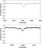 |
Fig. 8 Profiles of Hα and Pδ in HD 40111, B0.5 II. |
 |
Fig. 9 Profiles of Hα and Pδ in HD 91316, B1 Iab. |
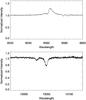 |
Fig. 10 Profiles of Hα and Pδ in HD 2905, B1 Iae. |
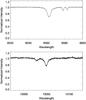 |
Fig. 11 Profiles of Hα and Pδ in D24398, B1 Ib. |
 |
Fig. 12 Profile of Pδ in HD 116658, B1 III. |
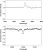 |
Fig. 13 Profiles of Hα and Pδ in HD 41117, B2 Iaev. |
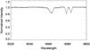 |
Fig. 14 Profile of Hα in HD 206165, B2 Ib. |
 |
Fig. 15 Profiles of Hα and Pδ in HD 886, B2 IV. |
 |
Fig. 16 Profiles of Hα and Pδ in HD 198478, B2.5 Ia. |
 |
Fig. 17 Profiles of Hα and Pδ in HD 35708, B2.5 IV. |
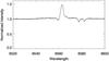 |
Fig. 18 Profile of Hα in HD 14143, B3 I. |
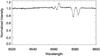 |
Fig. 19 Profile of Hα in HD 14134, B3 Ia. |
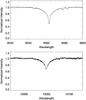 |
Fig. 20 Profiles of Hα and Pδ in HD 11415, B3 III. |
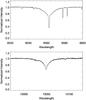 |
Fig. 21 Profiles of Hα and Pδ in HD 160762, B3 IV. |
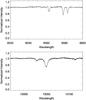 |
Fig. 22 Profiles of Hα and Pδ in HD 36371, B4 Ib. |
 |
Fig. 23 Profile of Hα in HD 15497, B6 Ia. |
 |
Fig. 24 Profiles of Hα and Pδ in HD 155763, B6 III. |
 |
Fig. 25 Profile of Hα in HD 3240, B7 III. |
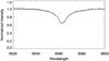 |
Fig. 26 Profile of Hα in HD 69686, B8. |
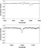 |
Fig. 27 Profiles of Hα and Pδ in HD 34085, B8 Iab. |
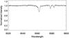 |
Fig. 28 Profile of Hα in HD 14322, B8 Ib. |
 |
Fig. 29 Profiles of Hα and Pδ in HD 63975, B8 II. |
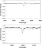 |
Fig. 30 Profiles of Hα and Pδ in HD 21291, B9 Ia. |
 |
Fig. 31 Profile of Hα in HD 212593, B9 Iab. |
 |
Fig. 32 Profiles of Hα and Pδ in HD 46300 (13 Mon) A0 Ib. |
 |
Fig. 33 Profiles of Hα and Pδ in HD 87737, A0 Ib. |
 |
Fig. 34 Profiles of Hα and Pδ in HD 47105, A0 IV. |
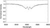 |
Fig. 35 Profile of Hα in HD 25642, A0 IVn. |
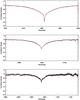 |
Fig. 36 Profiles of Hα, Pδ, and Pγ in HD 172167 (Vega) A0 V. |
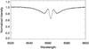 |
Fig. 37 Profile of Hα in HD 34787, A0 Vne. |
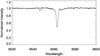 |
Fig. 38 Profile of Hα in HD 14433, A1 Ia. |
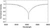 |
Fig. 39 Profile of Hα in HD 214994, A1 IV. |
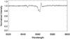 |
Fig. 40 Profile of Hα in HD 14489, A2 Ia. |
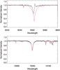 |
Fig. 41 Profiles of Hα and Pδ in HD 197345 (Deneb) A2 Iae. |
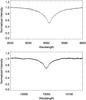 |
Fig. 42 Profiles of Hα and Pδ in HD 50019, A3 III. |
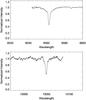 |
Fig. 43 Profiles of Hα and Pδ in HD 17378, A5 Ia. The limited wavelength coverage is due to the display of one order of the echelle. |
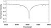 |
Fig. 44 Profile of Hα in HD 2628, A7 III. |
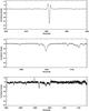 |
Fig. 45 Profiles of Hα, Pδ, and Pγ in HD 31964, A8 Iab. |
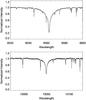 |
Fig. 46 Profiles of Hα and Pδ in HD 182835, F2 Iab. |
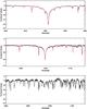 |
Fig. 47 Profiles of Hα, Pδ, and Pγ in HD 20902 (αPer) F5 Iab. |
 |
Fig. 48 Profile of Pδ in HD 213306, F5 Iab. |
 |
Fig. 49 Profile of Pδ in HD 187929, F6 Iab. |
 |
Fig. 50 Profile of Hα in HD 33564, F6 V. |
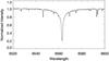 |
Fig. 51 Profile of Hα in HD 215648, F7 V. |
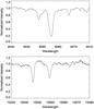 |
Fig. 52 Profiles of Hα and Pδ in HD 18391, G0 Ia. |
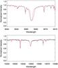 |
Fig. 53 Profiles of Hα and Pδ in HD 204867, G0 Ib. |
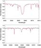 |
Fig. 54 Profiles of Hα and Pδ in HD 209750, G2 Ib. |
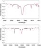 |
Fig. 55 Profiles of Hα and Pδ in HD 188727, G5 Ibv. |
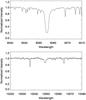 |
Fig. 56 Profiles of Hα and Pδ in HD 71369, G5 III. |
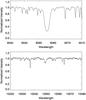 |
Fig. 57 Profiles of Hα and Pδ in HD 77912, G8 Ib-II. |
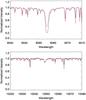 |
Fig. 58 Profiles of Hα and Pδ in HD 62345, G8 IIIa. |
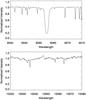 |
Fig. 59 Profiles of Hα and Pδ in HD 6833, G9 III. |
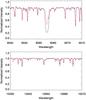 |
Fig. 60 Profiles of Hα and Pδ in HD 124897 (Arcturus) K1.5 III. |
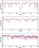 |
Fig. 61 Profiles of Hα, Pδ, and Pγ in HD 206778, K2 Ib. |
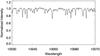 |
Fig. 62 Profile Pδ in HD 85503, K2 III. |
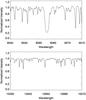 |
Fig. 63 Profiles of Hα and Pδ in HD 156283, K3 Iab. |
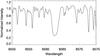 |
Fig. 64 Profile of Hα in HD 17506, K3 Ib. |
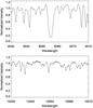 |
Fig. 65 Profiles of Hα and Pδ in HD 44537, K5 Iab. |
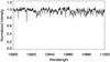 |
Fig. 66 Profile Pγ in HD 29139, K5 III. |
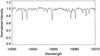 |
Fig. 67 Profile Pδ in HD 147767, K5 III. |
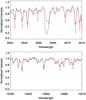 |
Fig. 68 Profiles of Hα and Pδ in HD 42543, M0 Iab. |
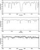 |
Fig. 69 Profiles of Hα, Pδ, and Pγ in HD 6860, M0 III. |
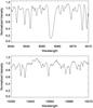 |
Fig. 70 Profiles of Hα and Pδ in HD 14330, M1 sd. |
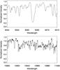 |
Fig. 71 Profiles of Hα and Pγ in HD 206936 (μCep) M2 Ia. |
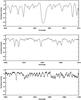 |
Fig. 72 Profiles of Hα, Pδ, and Pγ in HD 36389, M2 Iab. |
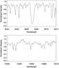 |
Fig. 73 Profiles of Hα and Pδ in HD 13136, M2 Iab. |
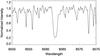 |
Fig. 74 Profile of Hα in HD 147749, M2 III. |
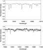 |
Fig. 75 Profiles of Pδ and Pγ in HD 217906, M2.5 II. |
 |
Fig. 76 Profile Pδ in HD 14469, M3 Iab. |
 |
Fig. 77 Profile of Pγ in HD 42995, M3 III. |
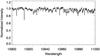 |
Fig. 78 Profile of Pγ in HD 44478, M3 III. |
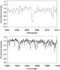 |
Fig. 79 Profiles of Hα and Pγ in HD 172380 (XY Lyr) M4 Iab. |
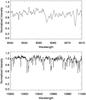 |
Fig. 80 Profiles of Hα and Pγ in HD 197812 (U Del) M5 Ia. |
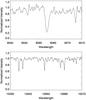 |
Fig. 81 Profiles of Hα and Pδ in HD 156014, M5 Ib-II. |
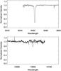 |
Fig. 82 Profiles of Hα and Pδ in HD 2796, F p. The limited wavelength coverage is due to the display of one order of the echelle. |
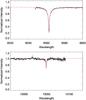 |
Fig. 83 Profiles of Hα and Pδ in HD 140283, F3 sd. The limited wavelength coverage is due to the display of one order of the echelle. |
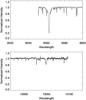 |
Fig. 84 Profiles of Hα and Pδ in HD 6755, F8 V. The limited wavelength coverage is due to the display of one order of the echelle. |
 |
Fig. 85 Profiles of Hα and Pδ in HD 221170, G2 IV. |
 |
Fig. 86 Profiles of Hα and Pδ in HD 216143, G5. |
 |
Fig. 87 Profiles of Hα and Pδ in HD 2665, G5 IIIp. |
 |
Fig. 88 Profiles of Hα and Pδ in BD+44 493, G5 IV. The limited wavelength coverage is due to the display of one order of the echelle. |
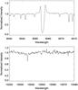 |
Fig. 89 Profiles of Hα and Pδ in HD 218732, G7 Ib. |
 |
Fig. 90 Profiles of Hα and Pδ in HD 187111, G8 p. |
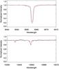 |
Fig. 91 Profiles of Hα and Pδ in HD 122563, K0 IIp. |
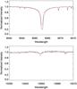 |
Fig. 92 Profiles of Hα and Pδ in HD 103095, K0 Vp. |
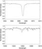 |
Fig. 93 Profiles of Hα and Pδ in HD 4306, K IIp. |
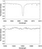 |
Fig. 94 Profiles of Hα and Pδ in HD 25329, K1 V. |
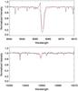 |
Fig. 95 Profiles of Hα and Pδ in HD 165195, K3p. |
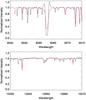 |
Fig. 96 Profiles of Hα and Pδ in HD 232078, K3 IIp. |
Acknowledgments
We thank David Bohlender, Les Saddlemyer, Dmitry Monin, Marilyn Bell and other DAO staff for their assistance in making these observations successful. We are also very grateful for the financial support of the Kenilworth Fund of the New York Community Trust. This research has made use of the SIMBAD database, operated at CDS, Strasbourg, France.
References
- Albayrak, B. 2000, A&A, 364, 237 [NASA ADS] [Google Scholar]
- Asplund, M. 2005, ARA&A, 43, 481 [NASA ADS] [CrossRef] [Google Scholar]
- Bakos, G. A. 1971, JRASC, 65, 222 [NASA ADS] [Google Scholar]
- Barzdis, A. 2010, MNRAS, 408, 1452 [NASA ADS] [CrossRef] [Google Scholar]
- Bergemann, M., & Gehren, T. 2008, A&A, 492, 823 [NASA ADS] [CrossRef] [EDP Sciences] [Google Scholar]
- Burris, D. L., Pilachowski, C. A., Armandroff, T. E., et al. 2000, ApJ, 544, 302 [NASA ADS] [CrossRef] [Google Scholar]
- Carr, J. S., Sellgren, K., & Balachandran, S. C. 2000, ApJ, 530, 307 [NASA ADS] [CrossRef] [Google Scholar]
- Cowley, C. R., & Castelli, F. 2002, A&A, 387, 595 [NASA ADS] [CrossRef] [EDP Sciences] [Google Scholar]
- Erspamer, D., & North, P. 2003, A&A, 398, 1121 [NASA ADS] [CrossRef] [EDP Sciences] [Google Scholar]
- Fernandez-Villacanas, J. L., Rego, M., & Cornide, M. 1990, AJ, 99, 1961 [NASA ADS] [CrossRef] [Google Scholar]
- Fuhrmann, K. 2008, MNRAS, 384, 173 [NASA ADS] [CrossRef] [Google Scholar]
- Fulbright, J. P. 2000, AJ, 120, 1841 [NASA ADS] [CrossRef] [Google Scholar]
- Gies, D. R., & Lambert, D. 1992, ApJ, 387, 673 [NASA ADS] [CrossRef] [Google Scholar]
- Gonzalez, G., Carlson, M. K., & Tobin, R. W. 2010, MNRAS, 403, 1368 [NASA ADS] [CrossRef] [Google Scholar]
- Hekker, S., & Meléndez, J. 2007, A&A, 475, 1003 [NASA ADS] [CrossRef] [EDP Sciences] [Google Scholar]
- Hill, G. M. 1995, A&A, 294, 536 [NASA ADS] [Google Scholar]
- Hui-Bon-Hoa, A. 2000, A&AS, 144, 203 [NASA ADS] [CrossRef] [EDP Sciences] [Google Scholar]
- Ito, H., Aoki, W., Honda, S., & Beers, T. C. 2009, ApJ, 698, L371 [NASA ADS] [CrossRef] [Google Scholar]
- Kurucz, R. L. 1993a, ATLAS9 Stellar Atmosphere Programs and 2 km s-1 grid, Kurucz CD-ROM No. 13 (Cambridge, Mass.: Smithsonian Astrophysical Observatory) [Google Scholar]
- Luck, R. E., & Bond, H. E. 1980, ApJ, 241, 218 [NASA ADS] [CrossRef] [Google Scholar]
- Luck, R. E., & Lambert, D. L. 1981, ApJ, 245, 1018 [NASA ADS] [CrossRef] [Google Scholar]
- Lyubimkov, L. S., Lambert, D. L., Rostopchin, S. I., Rachkovskaya, T. M., & Poklad, D. B. 2010, MNRAS, 402, 1369 [NASA ADS] [CrossRef] [Google Scholar]
- Mallik, S. V. 1998, A&A, 338, 623 [NASA ADS] [Google Scholar]
- McWilliam, A. 1990, ApJS, 74, 1075 [NASA ADS] [CrossRef] [Google Scholar]
- Meléndez, J., Asplund, M., Alves-Brito, A., et al. 2008, A&A, 484, 21 [Google Scholar]
- Mihalas, D., & Athay, R. G. 1973, ARA&A, 11, 187 [NASA ADS] [CrossRef] [Google Scholar]
- Mishenina, T. V., & Kovtyukh, V. V. 2001, A&A, 370, 951 [NASA ADS] [CrossRef] [EDP Sciences] [Google Scholar]
- Peters, G. J., & Aller, L. H. 1970, ApJ, 159, 525 [NASA ADS] [CrossRef] [Google Scholar]
- Przybilla, N., & Butler, K. 2004, ApJ, 610, 61 [Google Scholar]
- Sbordone, L. 2005, Mem. Soc. Astron. Ital. Suppl., 8, 61 [Google Scholar]
- Sbordone, L., Bonifacio, P., Castelli, F., & Kurucz, R. L. 2004, Mem. Soc. Astron. Ital. Suppl., 5, 93 [Google Scholar]
- Schuster, A. 1902, ApJ, 16, 320 [NASA ADS] [CrossRef] [Google Scholar]
- Schuster, A. 1905, ApJ, 21, 1 [NASA ADS] [CrossRef] [Google Scholar]
- Schwarzchild, K. 1906, Goettinger Nachr., 41 [Google Scholar]
- Smith, K. C., & Dworetsky, M. M. 1993, A&A, 274, 335 [NASA ADS] [Google Scholar]
- Smith, V. V., & Lambert, D. L. 1985, ApJ, 294, 326 [NASA ADS] [CrossRef] [Google Scholar]
- Spitzer, L. S. 1939, ApJ, 90, 494 [NASA ADS] [CrossRef] [Google Scholar]
- Struve, O., Wurm, K., & Henyey, L. G. 1939, PNAS, 25, 67 [NASA ADS] [CrossRef] [Google Scholar]
- Unsöld, A., & Weidemann, V. 1955, VA, 1, 249 [NASA ADS] [Google Scholar]
- van Leeuwen, F. 2007, A&A, 474, 653 [NASA ADS] [CrossRef] [EDP Sciences] [Google Scholar]
- Venn, K. A. 1995, ApJS, 99, 659 [NASA ADS] [CrossRef] [Google Scholar]
- Vidal, C. R., Cooper, J., & Smith, E. W. 1973, ApJS, 25, 37 [NASA ADS] [CrossRef] [Google Scholar]
All Tables
All Figures
|
Fig. 1 Profiles for Hα, Pδ, and Pγ (a), b) and c) respectively) in HD 39801 (αOri) M2 Iab. The black line is the observed spectrum and the red line is the model spectrum. |
| In the text | |
|
Fig. 2 Profiles of Hαa)–f) and Pδg)–l) for selected stars of high luminosity. |
| In the text | |
|
Fig. 3 Profiles of Hαa)–f) and Pδg)–l) for selected stars of high luminosity. |
| In the text | |
|
Fig. 4 Profiles of Hαa)–e) and Pδg)–k) for selected spectral type K stars. |
| In the text | |
|
Fig. 5 Profiles of Pγ for select stars. |
| In the text | |
|
Fig. 6 HD 172167 (Vega) A0 V: except for a very small deviation at the center of the Hα profile, this fundamental standard for modelling stellar atmospheres shows a very good fit between the modelled and the observed profiles for Hα and Pδ. |
| In the text | |
|
Fig. 7 Profiles of Hα and Pδ in HD 37128, B0 Iab. |
| In the text | |
|
Fig. 8 Profiles of Hα and Pδ in HD 40111, B0.5 II. |
| In the text | |
|
Fig. 9 Profiles of Hα and Pδ in HD 91316, B1 Iab. |
| In the text | |
|
Fig. 10 Profiles of Hα and Pδ in HD 2905, B1 Iae. |
| In the text | |
|
Fig. 11 Profiles of Hα and Pδ in D24398, B1 Ib. |
| In the text | |
|
Fig. 12 Profile of Pδ in HD 116658, B1 III. |
| In the text | |
|
Fig. 13 Profiles of Hα and Pδ in HD 41117, B2 Iaev. |
| In the text | |
|
Fig. 14 Profile of Hα in HD 206165, B2 Ib. |
| In the text | |
|
Fig. 15 Profiles of Hα and Pδ in HD 886, B2 IV. |
| In the text | |
|
Fig. 16 Profiles of Hα and Pδ in HD 198478, B2.5 Ia. |
| In the text | |
|
Fig. 17 Profiles of Hα and Pδ in HD 35708, B2.5 IV. |
| In the text | |
|
Fig. 18 Profile of Hα in HD 14143, B3 I. |
| In the text | |
|
Fig. 19 Profile of Hα in HD 14134, B3 Ia. |
| In the text | |
|
Fig. 20 Profiles of Hα and Pδ in HD 11415, B3 III. |
| In the text | |
|
Fig. 21 Profiles of Hα and Pδ in HD 160762, B3 IV. |
| In the text | |
|
Fig. 22 Profiles of Hα and Pδ in HD 36371, B4 Ib. |
| In the text | |
|
Fig. 23 Profile of Hα in HD 15497, B6 Ia. |
| In the text | |
|
Fig. 24 Profiles of Hα and Pδ in HD 155763, B6 III. |
| In the text | |
|
Fig. 25 Profile of Hα in HD 3240, B7 III. |
| In the text | |
|
Fig. 26 Profile of Hα in HD 69686, B8. |
| In the text | |
|
Fig. 27 Profiles of Hα and Pδ in HD 34085, B8 Iab. |
| In the text | |
|
Fig. 28 Profile of Hα in HD 14322, B8 Ib. |
| In the text | |
|
Fig. 29 Profiles of Hα and Pδ in HD 63975, B8 II. |
| In the text | |
|
Fig. 30 Profiles of Hα and Pδ in HD 21291, B9 Ia. |
| In the text | |
|
Fig. 31 Profile of Hα in HD 212593, B9 Iab. |
| In the text | |
|
Fig. 32 Profiles of Hα and Pδ in HD 46300 (13 Mon) A0 Ib. |
| In the text | |
|
Fig. 33 Profiles of Hα and Pδ in HD 87737, A0 Ib. |
| In the text | |
|
Fig. 34 Profiles of Hα and Pδ in HD 47105, A0 IV. |
| In the text | |
|
Fig. 35 Profile of Hα in HD 25642, A0 IVn. |
| In the text | |
|
Fig. 36 Profiles of Hα, Pδ, and Pγ in HD 172167 (Vega) A0 V. |
| In the text | |
|
Fig. 37 Profile of Hα in HD 34787, A0 Vne. |
| In the text | |
|
Fig. 38 Profile of Hα in HD 14433, A1 Ia. |
| In the text | |
|
Fig. 39 Profile of Hα in HD 214994, A1 IV. |
| In the text | |
|
Fig. 40 Profile of Hα in HD 14489, A2 Ia. |
| In the text | |
|
Fig. 41 Profiles of Hα and Pδ in HD 197345 (Deneb) A2 Iae. |
| In the text | |
|
Fig. 42 Profiles of Hα and Pδ in HD 50019, A3 III. |
| In the text | |
|
Fig. 43 Profiles of Hα and Pδ in HD 17378, A5 Ia. The limited wavelength coverage is due to the display of one order of the echelle. |
| In the text | |
|
Fig. 44 Profile of Hα in HD 2628, A7 III. |
| In the text | |
|
Fig. 45 Profiles of Hα, Pδ, and Pγ in HD 31964, A8 Iab. |
| In the text | |
|
Fig. 46 Profiles of Hα and Pδ in HD 182835, F2 Iab. |
| In the text | |
|
Fig. 47 Profiles of Hα, Pδ, and Pγ in HD 20902 (αPer) F5 Iab. |
| In the text | |
|
Fig. 48 Profile of Pδ in HD 213306, F5 Iab. |
| In the text | |
|
Fig. 49 Profile of Pδ in HD 187929, F6 Iab. |
| In the text | |
|
Fig. 50 Profile of Hα in HD 33564, F6 V. |
| In the text | |
|
Fig. 51 Profile of Hα in HD 215648, F7 V. |
| In the text | |
|
Fig. 52 Profiles of Hα and Pδ in HD 18391, G0 Ia. |
| In the text | |
|
Fig. 53 Profiles of Hα and Pδ in HD 204867, G0 Ib. |
| In the text | |
|
Fig. 54 Profiles of Hα and Pδ in HD 209750, G2 Ib. |
| In the text | |
|
Fig. 55 Profiles of Hα and Pδ in HD 188727, G5 Ibv. |
| In the text | |
|
Fig. 56 Profiles of Hα and Pδ in HD 71369, G5 III. |
| In the text | |
|
Fig. 57 Profiles of Hα and Pδ in HD 77912, G8 Ib-II. |
| In the text | |
|
Fig. 58 Profiles of Hα and Pδ in HD 62345, G8 IIIa. |
| In the text | |
|
Fig. 59 Profiles of Hα and Pδ in HD 6833, G9 III. |
| In the text | |
|
Fig. 60 Profiles of Hα and Pδ in HD 124897 (Arcturus) K1.5 III. |
| In the text | |
|
Fig. 61 Profiles of Hα, Pδ, and Pγ in HD 206778, K2 Ib. |
| In the text | |
|
Fig. 62 Profile Pδ in HD 85503, K2 III. |
| In the text | |
|
Fig. 63 Profiles of Hα and Pδ in HD 156283, K3 Iab. |
| In the text | |
|
Fig. 64 Profile of Hα in HD 17506, K3 Ib. |
| In the text | |
|
Fig. 65 Profiles of Hα and Pδ in HD 44537, K5 Iab. |
| In the text | |
|
Fig. 66 Profile Pγ in HD 29139, K5 III. |
| In the text | |
|
Fig. 67 Profile Pδ in HD 147767, K5 III. |
| In the text | |
|
Fig. 68 Profiles of Hα and Pδ in HD 42543, M0 Iab. |
| In the text | |
|
Fig. 69 Profiles of Hα, Pδ, and Pγ in HD 6860, M0 III. |
| In the text | |
|
Fig. 70 Profiles of Hα and Pδ in HD 14330, M1 sd. |
| In the text | |
|
Fig. 71 Profiles of Hα and Pγ in HD 206936 (μCep) M2 Ia. |
| In the text | |
|
Fig. 72 Profiles of Hα, Pδ, and Pγ in HD 36389, M2 Iab. |
| In the text | |
|
Fig. 73 Profiles of Hα and Pδ in HD 13136, M2 Iab. |
| In the text | |
|
Fig. 74 Profile of Hα in HD 147749, M2 III. |
| In the text | |
|
Fig. 75 Profiles of Pδ and Pγ in HD 217906, M2.5 II. |
| In the text | |
|
Fig. 76 Profile Pδ in HD 14469, M3 Iab. |
| In the text | |
|
Fig. 77 Profile of Pγ in HD 42995, M3 III. |
| In the text | |
|
Fig. 78 Profile of Pγ in HD 44478, M3 III. |
| In the text | |
|
Fig. 79 Profiles of Hα and Pγ in HD 172380 (XY Lyr) M4 Iab. |
| In the text | |
|
Fig. 80 Profiles of Hα and Pγ in HD 197812 (U Del) M5 Ia. |
| In the text | |
|
Fig. 81 Profiles of Hα and Pδ in HD 156014, M5 Ib-II. |
| In the text | |
|
Fig. 82 Profiles of Hα and Pδ in HD 2796, F p. The limited wavelength coverage is due to the display of one order of the echelle. |
| In the text | |
|
Fig. 83 Profiles of Hα and Pδ in HD 140283, F3 sd. The limited wavelength coverage is due to the display of one order of the echelle. |
| In the text | |
|
Fig. 84 Profiles of Hα and Pδ in HD 6755, F8 V. The limited wavelength coverage is due to the display of one order of the echelle. |
| In the text | |
|
Fig. 85 Profiles of Hα and Pδ in HD 221170, G2 IV. |
| In the text | |
|
Fig. 86 Profiles of Hα and Pδ in HD 216143, G5. |
| In the text | |
|
Fig. 87 Profiles of Hα and Pδ in HD 2665, G5 IIIp. |
| In the text | |
|
Fig. 88 Profiles of Hα and Pδ in BD+44 493, G5 IV. The limited wavelength coverage is due to the display of one order of the echelle. |
| In the text | |
|
Fig. 89 Profiles of Hα and Pδ in HD 218732, G7 Ib. |
| In the text | |
|
Fig. 90 Profiles of Hα and Pδ in HD 187111, G8 p. |
| In the text | |
|
Fig. 91 Profiles of Hα and Pδ in HD 122563, K0 IIp. |
| In the text | |
|
Fig. 92 Profiles of Hα and Pδ in HD 103095, K0 Vp. |
| In the text | |
|
Fig. 93 Profiles of Hα and Pδ in HD 4306, K IIp. |
| In the text | |
|
Fig. 94 Profiles of Hα and Pδ in HD 25329, K1 V. |
| In the text | |
|
Fig. 95 Profiles of Hα and Pδ in HD 165195, K3p. |
| In the text | |
|
Fig. 96 Profiles of Hα and Pδ in HD 232078, K3 IIp. |
| In the text | |
Current usage metrics show cumulative count of Article Views (full-text article views including HTML views, PDF and ePub downloads, according to the available data) and Abstracts Views on Vision4Press platform.
Data correspond to usage on the plateform after 2015. The current usage metrics is available 48-96 hours after online publication and is updated daily on week days.
Initial download of the metrics may take a while.