| Issue |
A&A
Volume 546, October 2012
|
|
|---|---|---|
| Article Number | A56 | |
| Number of page(s) | 12 | |
| Section | Planets and planetary systems | |
| DOI | https://doi.org/10.1051/0004-6361/201219297 | |
| Published online | 04 October 2012 | |
Modeled flux and polarization signals of horizontally inhomogeneous exoplanets applied to Earth-like planets
1
SRON – Netherlands Institute for Space Research,
Sorbonnelaan 2,
3584 CA
Utrecht,
The Netherlands
e-mail: T.Karalidi@sron.nl
2
Leiden Observatory, PO Box 9513, 2300 RA, Leiden, The Netherlands
Received: 28 March 2012
Accepted: 30 August 2012
Aims. We present modeled flux and linear polarization signals of starlight that is reflected by spatially unresolved, horizontally inhomogeneous planets and discuss the effects of including horizontal inhomogeneities on the flux and polarization signals of Earth-like exoplanets.
Methods. Our code is based on an efficient adding-doubling algorithm, which fully includes multiple scattering by gases and aerosol/cloud particles. We divide a model planet into pixels that are small enough for the local properties of the atmosphere and surface (if present) to be horizontally homogeneous. Given a planetary phase angle, we sum up the reflected total and linearly polarized fluxes across the illuminated and visible part of the planetary disk, taking care to properly rotate the polarized flux vectors towards the same reference plane.
Results. We compared flux and polarization signals of simple horizontally inhomogeneous model planets against results of the weighted sum approximation, in which signals of horizontally homogeneous planets are combined. Apart from cases in which the planet has only a minor inhomogeneity, the signals differ significantly. In particular, the shape of the polarization phase function appears to be sensitive to the horizontal inhomogeneities. The same holds true for Earth-like model planets with patchy clouds above an ocean and a sandy continent. Our simulations clearly show that horizontal inhomogeneities leave different traces in flux and polarization signals. Combining flux with polarization measurements would help retrieving the atmospheric and surface patterns on a planet.
Key words: planets and satellites: atmospheres / methods: numerical / polarization / planets and satellites: surfaces
© ESO, 2012
1. Introduction
Since Mayor & Queloz (1995) discovered the first planet orbiting another main sequence star almost two decades ago, the rapid improvement of detection methods and instruments has yielded hundreds of exoplanets, including several tens of so-called super-Earths (see e.g. Léger et al. 2011; Charbonneau et al. 2009; Miller-Ricci & Fortney 2010; Beaulieu et al. 2006), and many more will follow in the coming years. The next step in exoplanet research is the characterization of the atmospheres and surfaces (if present) of detected exoplanets: what is their composition and structure?
Currently, exoplanet atmospheres are being characterized using the transit method (see e.g. Beaulieu et al. 2010; Miller-Ricci & Fortney 2010). This method is based on measurements of the wavelength dependendence of starlight that filters through the upper planetary atmosphere during the primary transit, or of the planetary flux just before or after the secondary eclipse. The transit method is mostly applied to gaseous planets that orbit close to their star. The chances to catch gaseous planets in wide orbits, such as Jupiter and Saturn in our solar system, transiting their star are extremely small, because their orbital plane should be perfectly aligned with our line of sight and because their transits are very rare. Earth-sized exoplanets in the habitable zone of a solar-type star are probably too small and transit too seldom to reach a sufficient signal-to-noise ratio to do transit spectroscopy (Kaltenegger & Traub 2009).
A promising method to characterize atmospheres and surfaces (if present) of exoplanets that are small and/or in wide orbits, is direct detection, in which the starlight that a planet reflects and/or the thermal radiation that a planet emits is measured separately from the stellar light (except for some background starlight). Some instruments that are being designed for such direct detections are SPHERE (for the VLT) and EPICS (for the European Extremely Large Telescope, or E-ELT). An example for a space telescope for direct detection is the New Worlds Observer (NWO; Cash & New Worlds Study Team 2010), which is under study by NASA. Through direct detections, broadband images and/or spectra of various types of exoplanets will become available in the near future.
Knowing the solar system planets, it is to be expected that exoplanets that will be observed are horizontally inhomogeneous, e.g. with clouds and hazes in patches, such as on Earth and Mars, or in banded structures, such as, for example, on Jupiter and Saturn. And there will undoubtedly be solid exoplanets with significant local variations in surface reflection properties and texture, such as the Earth with its continents and oceans. Although the lack of spatial resolution in near future exoplanet observations will merge all spatial variation into a single image pixel and/or spectrum, accounting for the existence of horizontal inhomogeneities will be important when trying to retrieve planet characteristics. For example, efforts to identify spectral signatures of life on other planets will face various challenges, such as clouds masking or mimicking the signatures of vegetation (Tinetti et al. 2006, and references therein). The cloud coverage will also influence the retrieval of mixing ratios of atmospheric gases, such as water vapour and oxygen, from reflected light spectra. In particular, the larger the fraction of clouds across an exoplanetery surface, the smaller the depth of gaseous absorption bands. Absorption band depths are, however, also influenced by the cloud top altitudes, with higher clouds yielding shallower absorption bands (for examples, see Stam 2008). The distribution of cloud top altitudes across a planet will thus also be a parameter to take into account.
Horizontal inhomogenities can have large effects on the flux of starlight that is reflected by a planet. In particular, Ford et al. (2001) have shown that an Earth analogue planet without clouds would show diurnal flux variations of up to 150% due to the variation of the albedo of different regions on the planet. In full agreement, Oakley & Cash (2009) have calculated that in absence of an atmosphere, the flux of an Earth-like exoplanet would show a clear diurnal variability as different continents would rotate in and out of the field of view of an observer. The presence of clouds in the Earth’s atmosphere significantly complicates the characterization of various surface types. Ford et al. (2001) show, for example, that an Earth-like cloud pattern would suppress the diurnal flux variations to as little as 20%, while Oakley & Cash (2009) indicate that characterizing the surface of the planet is possible only for cloud coverages significantly lower than the average coverage on Earth (≲ 25% versus ~60%). To quantitatively estimate the effects of horizontal inhomogeneities due to clouds or surface features on observed spectra, and to be able to account for such variations in the retrieval of planet characteristics from future observations, numerical codes are essential tools.
In this paper, we present our numerical code to calculate spectra of starlight that is reflected by spatially unresolved, horizontally inhomogeneous exoplanets. The main difference with other codes for horizontally inhomogeneous planets (such as those used by Ford et al. 2001; Oakley & Cash 2009; Tinetti et al. 2006) is that it can be used to calculate not only the flux of reflected starlight but also its state (degree and direction) of polarization. Polarimetry promises to play an important role in exoplanet research both for exoplanet detection and characterization. In particular, because the direct starlight is unpolarized, while the starlight that is reflected by a planet will usually be polarized (see e.g. Zugger et al. 2010; Stam et al. 2006, 2004; Saar & Seager 2003; Seager et al. 2000), polarimetry can increase the planet-to-star contrast ratio by 3 to 4 orders of magnitude (Keller et al. 2010), thus facilitating the detection of an exoplanet that might otherwise be lost in the glare of its parent star. Polarimetry will not only help to detect a planet, it will also confirm the status of the object, since background objects will usually be unpolarized.
The importance of polarimetry for studying planetary atmospheres and surfaces has been shown many times using observations of the Earth and other solar system planets (see for example Hansen & Hovenier 1974; Hansen & Travis 1974; Mishchenko 1990; Tomasko et al. 2009), as well as by modeling of solar system planets or giant exoplanets (e.g. Madhusudhan & Burrows 2012; Stam 2008, 2003; Stam et al. 2004; Saar & Seager 2003; Seager et al. 2000). In particular, the sensitivity of polarization to the microphysical properties of the scatterers in the planetary atmosphere, make it a crucial tool for braking degeneracies that flux only observations can have.
The radiative transfer calculations in our code are based on an efficient adding-doubling algorithm (de Haan et al. 1987) which fully includes multiple scattering by gases and aerosol/cloud particles, that was used before for flux and polarization calculations for gaseous and terrestrial exoplanets by Stam (2003); Stam et al. (2004, 2008); Karalidi et al. (2011). These authors, however, assumed each exoplanet to be horizontally homogeneous, such that it could be treated as a single starlight scattering “particle”, which allowed for a very fast integration of the reflected flux and polarization signals across the planet’s disk for the whole planetary phase angle range (see Stam et al. 2006, for a description of this disk-integration algorithm). With this horizontally homogeneous code, the signals of horizontally inhomogeneous planets can be simulated using the so-called weighted sum approximation: signals of homogeneous planets are multiplied by a weighting factor and summed to yield the final signal. We, on the other hand, divide a horizontally inhomogeneous model planet into pixels that are small enough for the local properties of the atmosphere and surface (if present) to be horizontally homogeneous. For each type of pixel, we perform adding-doubling radiative transfer calculations (de Haan et al. 1987) and, given the planetary phase angle, we sum up the reflected total and polarized fluxes across the illuminated and visible part of the planetary disk. Our code for horizontally inhomogeneous planets allows investigating the applicability of the weighted sum approximation, and the effects of horizontal inhomogeneities on the flux and in particular the polarization signals of exoplanets.
This paper is organized as follows. In Sect. 2, we describe our numerical method to calculate the flux and polarization of starlight that is reflected by a horizontally inhomogeneous planet, and in Sect. 3, we present simulations of flux and polarization for different types of horizontal inhomogeneities. In Sect. 4, we present flux and polarization signals of horizontally inhomogeneous Earth-like planets and compare them to signals for horizontally homogeneous planets. Finally, in Sect. 5, we discuss and summarize our results. Appendix A contains the results of testing our code for horizontally inhomogeneous planets against an existing code for horizontally homogeneous planets.
2. Calculating reflected starlight
Light can fully be described by a flux vector πF, as follows ![\begin{equation} \pi\vec{F}= \pi \left[\begin{array}{c} F \\ Q \\ U \\ V \end{array}\right], \label{eq:first} \end{equation}](/articles/aa/full_html/2012/10/aa19297-12/aa19297-12-eq6.png) (1)with πF the total, πQ and πU the linearly and πV the circularly polarized fluxes (see e.g. Hansen & Travis 1974; Hovenier et al. 2004; Stam 2008). Parameters πF, πQ, πU and πV depend on the wavelength λ, and have dimensions W m-2 m-1. Parameters πQ and πU are defined with respect to a reference plane, for which we choose the planetary scattering plane, i.e. the plane through the centers of the planet, star and observer. Note that this plane is usually not the same as the planetary orbital plane; only for orbits that are seen edge-on, the two planes coincide at all phase angles. In the following, we will ignore πV, because it is usually very small (Hansen & Travis 1974), and because the errors in calculated values of πF, πQ, and πU due to ignoring πV are negligible (Stam & Hovenier 2005).
(1)with πF the total, πQ and πU the linearly and πV the circularly polarized fluxes (see e.g. Hansen & Travis 1974; Hovenier et al. 2004; Stam 2008). Parameters πF, πQ, πU and πV depend on the wavelength λ, and have dimensions W m-2 m-1. Parameters πQ and πU are defined with respect to a reference plane, for which we choose the planetary scattering plane, i.e. the plane through the centers of the planet, star and observer. Note that this plane is usually not the same as the planetary orbital plane; only for orbits that are seen edge-on, the two planes coincide at all phase angles. In the following, we will ignore πV, because it is usually very small (Hansen & Travis 1974), and because the errors in calculated values of πF, πQ, and πU due to ignoring πV are negligible (Stam & Hovenier 2005).
The degree of polarization P of vector πF is defined as  (2)which is independent of the choice of reference plane. For planets that are mirror-symmetric with respect to the planetary scattering plane (e.g. horizontally homogeneous planets), Stokes parameter U equals zero. In that case, we can use an alternative definition of the degree of polarization
  (3)with the sign indicating the direction of the polarization, i.e. if Ps > 0 (Ps < 0) the light is polarized perpendicular (parallel) to the planetary scattering plane. The absolute value of Ps is just equal to P.
We calculate the flux vector of starlight that has been reflected by a spherical planet with radius r at a distance d from the observer using (d ≫ r) as (see Stam et al. 2006)  (4)with α the planetary phase angle, i.e. the angle between the star and the observer as seen from the planet’s center. Furthermore, πF0 is the flux vector of the incident starlight and S the 4 × 4 planetary scattering matrix. In the following, we normalize Eq. (4) assuming r = 1 and d = 1.
As described in Stam et al. (2006), the planetary scattering matrix S can be calculated by integrating local reflection matrices R across the illuminated and visible part of the planetary disk, as follows  (5)where dO is a surface element on the planet, and R is the local reflection matrix, which describes how starlight that is incident on a given location of the planet is reflected towards the observer. The reference planes for R are the local meridian planes, which contain the direction of propagation of the incident and reflected light, respectively, and the local vertical direction. The matrices L are so-called rotation matrices (see Hovenier et al. 2004; Hovenier & van der Mee 1983) that are used to rotate from the planetary scattering plane to the local meridian planes and back:
 ![\begin{eqnarray} \label{eq:matL} \vec{L}(\beta) = \left[\begin{array} {c c c c} 1 & 0 &0 &0 \\ 0& \cos2\beta &\sin2\beta & 0 \\ 0 & -\sin2\beta & \cos2\beta & 0 \\ 0 & 0 & 0 & 1\end{array} \right], \end{eqnarray}](/articles/aa/full_html/2012/10/aa19297-12/aa19297-12-eq36.png) (6)angle β is measured in the anti-clockwise direction from the old to the new reference plane when looking in the direction of propagation of the light.
(6)angle β is measured in the anti-clockwise direction from the old to the new reference plane when looking in the direction of propagation of the light.
In Eq. (5), we assume that the planetary atmosphere and surface (if present) are locally plane-parallel and rotationally symmetric with respect to the local vertical direction. Therefore, each matrix R depends on μ0 = cosθ0, with θ0 the angle between the local zenith and the direction towards the star, on μ = cosθ, with θ the angle between the local zenith and the direction towards the observer, and on Δφ = φ − φ0, the angle between the azimuthal angles of the incident and the reflected light, respectively. Azimuthal angles are measured rotating clockwise when looking up from an arbitrary, local vertical plane towards the local vertical plane containing the direction of propagation of the light.
For horizontally homogeneous planets, Stam et al. (2006) present an efficient method for evaluating Eq. (5) that uses an adding-doubling radiative transfer algorithm (de Haan et al. 1987) to calculate the coefficients of the expansion of the local reflection matrix (which is the same across the planet) into a Fourier series. These coefficients are then used to compute coefficients of the expansion of matrix S into generalized spherical functions. With these expansion coefficients, S can be calculated rapidly for any phase angle α. Since with this method, a planet is basically treated as a single light-scattering particle, it cannot be used for horizontally inhomogeneous planets.
To calculate S for horizontally inhomogeneous planets, we divide a planet into pixels small enough for the local atmosphere and surface (if present) to be considered both plane-parallel and horizontally homogeneous. For each type of pixel (a combination of surface and atmosphere properties), we first calculate the coefficients of the expansion of the local reflection matrix R into a Fourier series, using the adding-doubling algorithm (de Haan et al. 1987). Then, for each given planetary phase angle and each pixel, we use the respective Fourier coefficients to calculate the local reflection matrices (see de Haan et al. 1987). The local matrices are summed up according to  (7)with N the total number of pixels on the illuminated and visible part of the planetary disk.
In the following, we assume unpolarized incident starlight, since integrated over the stellar disk, light of solar-type stars can be assumed to be unpolarized (Kemp et al. 1987). In this case, πF0 = πF01, with 1 the unit column vector and πF0 the total incident stellar flux (measured perpendicular to the propagation direction of the light), for which we assume a normalized value of 1 W m-2 m-1. Thanks to the assumption of unpolarized incident starlight, rotation matrix L(β1i) can be ignored in Eq. (7).
Because of the normalizations and the assumption of unpolarized incident light, the total flux that is reflected by a planet (cf. Eq. (4)) is given by  (8)with a11 the (1, 1)-element of matrix S (see Stam 2008; Karalidi et al. 2011). The subscript n indicates the normalization. When α = 0°, the hence normalized total flux equals the planet’s geometric albedo AG. Our normalized total and polarized fluxes πFn, πQn and πUn can straightforwardly be scaled to any given planetary system using Eq. (4) and inserting the appropriate values for r, d and πF0. The degree of polarization (P or Ps) is independent of r, d and πF0, and would thus not require any scaling.
We have tested our disk-integration code by comparing its results with those of the code for horizontally homogeneous planets by Stam et al. (2006, see Appendix A). We have not compared it against other codes for modelling signals of horizontally inhomogeneous planets (see e.g. Ford et al. 2001; Oakley & Cash 2009; Tinetti et al. 2006), because these codes ignore polarization, which is the most interesting feature of our code. A comparison between calculated total fluxes would require us to disable the polarization calculations in our adding-doubling code, since ignoring polarization introduces errors of up to several percent in total flux calculations (Stam & Hovenier 2005). From the comparison with the code for horizontally homogeneous planets applied to horizontally inhomogeneous planets using the weighted sum approximation, in which weighted sums of flux vectors reflected by horizontally homogeneous planets are used to approximate the flux vectors of horizontally inhomogeneous planets (see Appendix A), we conclude that our code is accurate enough for application to horizontally inhomogeneous planets, provided enough pixels are used across the disk, not only for resolving the spatial variations but also the variations in illumination and viewing angles across pixels.
3. Sensitivity to horizontal inhomogeneities
In this section, we present flux and polarization (degree and angle) signals of planets with different types of horizontal inhomogeneities on their surfaces as calculated using our code to show the signatures of inhomogeneities and the differences with signatures of horizontally homogeneous planets with similar surface albedos. Unless stated otherwise, each planet has a gaseous, Rayleigh scattering atmosphere with a total optical thickness of ~0.1 (no absorption), and a flat surface. For the surface albedo, we choose the extreme values of 0.0 (black) and 1.0 (white), since they give the largest contrast in flux and polarization.
Establishing which types of inhomogeneities could still be handled with e.g. a weighted sum approximation and which would need a full scale horizontally inhomogeneous approach with e.g. our code (from hereon: the HI-code), is interesting for saving computing time when possible. The disadvantage of our HI-code is namely the large amount of computing time it requires as compared to the horizontally homogeneous code (HH-code) of Stam et al. (2006). For example, the HI-code takes about 105 times more time than the HH-code for calculating the flux vectors of a horizontally homogeneous planet covered by a cloud layer with optical thickness 2, for phase angles α from 0° to 180° in steps of 2°, with the planet having been divided into pixels of 2° × 2°, and for a single wavelength.
The difference in computation times would be irrelevant if the computing time of the HI-code were negligible. Unfortunately this is not the case. This time depends strongly on the properties of the model atmosphere, especially on the absorption and scattering optical thickness of the gases and particles in the atmosphere and on the angular variation of the single scattering properties of the scattering particles. In particular adding polarization to the flux calculations increases the time by at least an order of magnitude, and of course, the timing increases almost linearly with the number of wavelengths at which calculations are required (since these calculations are independent of each other, they could easily be done in parallel). For the cloudy model planet calculations described in the previous paragraph, the HH-code takes about a minute on an average workstation.
The difference in computing time is not spent in the radiative transfer calculations themselves, since the two codes use the same adding-doubling radiative transfer algorithm (based on de Haan et al. 1987) and were run with the same numerical accuracy. Also, because both planets were horizontally homogeneous, the radiative transfer calculation had to be performed only once for each code. Indeed, in the HI-code, the additional computing time is mostly spent in the integration of the flux vectors across the planetary disk. In particular, for α = 0°, the number of 2° × 2° pixels across the disk is more than 8000. For each pixel, the appropriate Fourier coefficients have to be determined from the list of calculated coefficients, they have to be summed to calculate the local reflection matrix, and with that the locally reflected flux vectors. Then, the locally reflected flux vectors have to be rotated to the planetary scattering plane in order to be summed up to calculate the reflected flux vector of the planet. Even though the computing time per pixel can be relatively small, the mere number of pixels (which of course depends on the planetary phase angle) can result in long computing times.
3.1. Planets with spots
The first type of horizontally inhomogeneous planets have black surfaces with homogeneously distributed white spots. We start with spots consisting of single white pixels that cover 4% of the planet’s surface, and let the area of each spot grow until the spots cover 68% of the surface. Figure 1 shows πFn and Ps (see Eq. (3)) as calculated using the HI-code as functions of the planetary phase angle α for these planets. As can be seen, increasing the percentage of white pixels from 4% to 68%, increases πFn smoothly from 0.09 to 0.58 at α = 0°, while Ps decreases from 0.6 to 0.08 at α = 90° (this phase angle does not coincide with the maximum of Ps). With increasing surface brightness, the peak value of Ps shifts from α = 98° (4% white) to α = 116° (68% white).
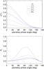 |
Fig. 1 πFn and Ps as functions of α for black, cloud-free planets with white spots occupying 4% (red, dotted line), 21% (green, dashed line), 41% (blue, dashed-dotted line), 57% (grey, dashed-triple-dotted line) and 68% (purple, long-dashed line) of the planet. |
Figure 2 shows the difference between the results from the HI-code and those from the HH-code (the latter combined with with the weighted sum approximation, as described in Appendix A). In Fig. 2, it is clear that when the planet is almost horizontally homogeneous (only 4% covered by white pixels), the maximum relative difference in flux, ΔπFn is very small (~0.64% for α = 0°), with the HI-code giving the slightly higher values. With increasing coverage, ΔπFn increases, showing a maximum value of 10% for 57% coverage in Fig. 2, to decrease again when the planet is almost homogeneously white.
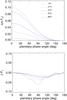 |
Fig. 2 Relative difference ΔπFn and the absolute difference ΔPs between the flux and polarization phase functions of the white spotted planets of Fig. 1 as calculated using the HI-code and the HH-code. The coverage of white spots is 4% (red, dotted line), 21% (green, dashed line), 41% (blue, dashed-dotted line), 57% (grey, dashed-tripple-dotted line) and 68% (purple, long-dashed line). |
Because the degree of polarization is itself a relative measure, we show the differences in Ps between the HI-code and the HH-code as absolute differences. As can be seen in Fig. 2, the absolute difference ΔPs is largest (~− 6% percent point around 90°) for the darkest planet and decreases towards the whiter planets. The HH-code produces at (almost) all phase angles a larger Ps than the HI-code. Interestingly, the polarization phase curve of the darkest planet is significantly less symmetrical when horizontally inhomogeneities are accurately taken into account (HI-code) than with the HH-code and the weighted sum approximation.
3.2. Planets with center continents
The second type of horizontally inhomogeneous planets have black surfaces and a circular “continent” of white pixels at the center of the planetary disk facing the observer (rotation of the planet, hence the rotation of the continent in and out of the field-of-view is not taken into account here). Figure 3 shows πFn and Ps as functions of α for planets with continents that cover from 5% to 98% of the disk. Both for the flux and the polarization, the curves for 80% and 98% coverage virtually overlap, because in these cases, the black pixels are all located along the limb of the planet and hardly contribute to the total signal. The flux phase functions in Fig. 3 have very similar shapes as those in Fig. 1, although the latter are darker for the same surface coverage of white pixels, which is not surprising since they have more black pixels on the front side of the disk. The polarization phase curves in Fig. 3 clearly have different, more asymmetrical shapes than those in Fig. 1, except for the largest coverages. The peak in the polarization phase curves indicates the phase angle where the continent disappears into the planet’s nightside.
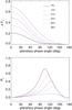 |
Fig. 3 πFn and Ps as functions of α for black, cloud-free planets with a white continent on the center of the planetary disk facing the observer, for different coverages of the continent: 5% (black, solid line), 12% (red, dashed line), 21% (blue, dashed-dotted line), 32% (green, dashed-triple-dotted line), 80% (magenta, long-dashed line) and 98% (gray, dotted line). |
Comparing the flux and polarization signals of the planets with white continents as calculated with our HI-code to the signals calculated using the HH-code (Fig. 4), it is obvious that the differences ΔπFn and ΔPs are smallest when the planetary disk is almost completely covered by the continent. In Fig. 4, the largest difference in the flux is about 33%, for a coverage of 32% and at α = 0°, with the HI-code giving the higher fluxes. The difference in polarization, ΔPs, clearly shows the strong asymmetry around α = 90° of Ps when calculated with the HI-code.
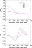 |
Fig. 4 ΔπFn and ΔPs between the phase functions of the white continent planets of Fig. 3 as calculated using the HI-code and the HH-code. The coverage of the continents is: 5% (black, solid line), 12% (red, dashed line), 21% (blue, dashed-dotted line), 32% (green, dashed-triple-dotted line), 80% (magenta, long-dashed line) and 98% (gray, dotted line) of the planetary disk. |
Figure 5 shows ΔπFn and ΔPs for the same planets except with a white surface and a black continent. Not surprisingly, for these planets, at most phase angles, πFn is smaller when calculated with the HI-code than with the HH-code for each percentage of coverage at most phase angles, because of the concentration of black pixels in the centre of the disk. The difference ΔPs is less asymmetric than for the black planets with white continents (cf. Fig. 3). The polarization phase functions as calculated using the two codes are thus similarly shaped. The maximum of the polarization phase function, however, does depend strongly on the code, and is thus sensitive to the distribution of pixels across the disk, with the HI-code yielding much higher maximum values of Ps than the HH-code, except for the smallest coverages. Indeed, for a white planet with a black continent covering 80% of the disk, Ps is almost 50% higher (around α = 80°) calculated with the HI-code than with the HH-code. Note that for this coverage, the difference in flux is relatively small (~− 10%) and similar to that for a coverage of 5%. The difference in sensitivity to the spatial distribution of albedo across the planetary disk between flux and polarization clearly illustrates the strengths of combined flux and polarization measurements.
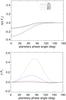 |
Fig. 5 Similar to Fig. 4, except for white, cloud-free planets with black continents. The coverage of the continents is: 5% (black, solid line), 21% (red, dashed line), 46% (blue, dashed-dotted line), and 80% (green, dashed-triple-dotted line) of the planetary disk. |
3.3. Planets with hemispherical caps
The third type of horizontally inhomogeneous planets have black surfaces and two, equally sized white caps on opposing sides of the planet. We will present results for three locations of the caps: 0° (the caps cover the “north” and the “south” poles of the planet), 45°, and 90° (the caps are on the “eastern” and “western” sides of the planetary disk). Planets with caps at 45° are not mirror-symmetric with respect to the planetary scattering plane. Therefore, Stokes parameter U will usually not be zero. In the following, we will therefore use Eq. (2) to define the degree of linear polarization instead of Eq. (3).
First, we’ll discuss the signals of planets with the caps covering the poles of the planets. Figure 6 shows πFn and P for different coverages of the caps as functions of α as calculated using the HI-code. The shape of the flux phase function is very smooth, and at α = 0°, πFn increases from 0.07 for 23% coverage, to 0.56 for 77% coverage. In the latter case, the planet is basically white with a black, equatorial belt (for a completely white planet, πFn would equal 0.7, see Fig. A.3). The polarization phase function is quite symmetric for small caps, and P decreases from almost 0.55 for 23% coverage to 0.08 for 77% coverage at α = 90° (note that the maxima of the polarization phase functions occur at somewhat smaller and larger phase angles, respectively).
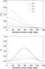 |
Fig. 6 πFn and P as functions of α for black, cloud-free planets with hemispherical caps occupying 23% (black, solid line), 43% (red, dashed line), 61% (blue, dashed-dotted line), and 77% (green, dashed-triple-dotted line) of the planet. The caps are located at the “north” and “south” poles of the planet. |
In Fig. 7, we show ΔπFn and ΔP for the planets in Fig. 6 when calculated using the HI-code and the HH-code. The difference in flux is negative for all values of α: the HI-code thus gives smaller fluxes than the HH-code for the same coverage. At α = 0°, ΔπFn is −0.14 for 23% coverage, increases up to −0.21 for 43% coverage, and decreases again to −0.07 for 77% coverage. In differences in polarization show that for small coverages, the HI-code gives significantly higher values of P than the HH-code. The reason is of course that for small coverages, the white pixels are mostly located near the limb of the planetary disk, where they contribute little to the total signal.
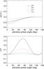 |
Fig. 7 ΔπFn and ΔPs between the phase functions of the capped planets of Fig. 6 as calculated using the HI-code and the HH-code. The caps occupy 23% (black, solid line), 43% (red, dashed line), 61% (blue, dashed-dotted line) and 77% (green, dashed-triple-dotted line) of the planet. |
Figure 8 shows πFn and P for planets with caps covering 23% of the disk for three different locations of the caps. The three different flux phase functions show the relatively small effects of different fractions of the caps being visible at a given phase angle. The polarization phase functions are all fairly symmetric around α = 90°, especially for the planet with its caps at the poles of the planet.
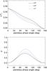 |
Fig. 8 πFn and P as functions of α for black, cloud-free planets with white, hemispherical caps that occupy 23% of the planet. The locations of the caps are: 0° (black, solid line), indicating the caps are on the “north” and “south” poles of the planet, 45° (red, dashed line), and 90° (blue, dashed-dotted line), with the caps on the “eastern” and “western” sides of the planetary disk. |
Figure 9 shows ΔπFn and ΔP for the three model planets of Fig. 8 as calculated using the HH-code and the HI-code. As can be seen, the ΔπFn are fairly independent of the caps’ position angle. This implies that it would be difficult to retrieve information about the position of the caps from the flux alone. Polarization appears to be more sensitive to the location of the caps. In particular, the ΔP are several percentage points depending on the location and on α. Around α = 90°, where exoplanets have a relatively high chance of being observed with direct detection methods, the differences in ΔP are about 0.12 for the planet with the eastern and western caps, implying that the accuracy of the polarimetry should be larger than 0.10 to be able to establish their existence.
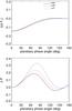 |
Fig. 9 ΔπFn and ΔPs between the phase functions of the capped planets of Fig. 8 as calculated using the HI-code and the HH-code. The cap locations are: 0° (black, solid line), 45° (red, dashed line), and 90° (blue, dashed-dotted line). |
4. Application to Earth-like planets
In this section, we present flux and polarization signals of planets with horizontally inhomogeneous Earth-like surface coverages and patchy cloud layers. In reality, the Earth exhibits a large variation in atmospheric temperature and pressure profiles, cloud properties (both on macro- and micro-scales) and surface properties. To avoid introducing too many variables, we assume a single temperature and pressure profile across our model planet, the so-called mid-latitude summer profile from McClatchey et al. (1972), a single type of cloud particles and cloud properties (optical thickness and vertical distribution), and a surface that is covered by either ocean or sand (a continent).
4.1. Surface inhomogeneities
First, we present the signals of a planet with a sandy continent surrounded by ocean. The continent extends between longitudes of ±22° and latitudes of ±50° (measured with respect to the subobserver point). The sand surface reflects Lambertian (unpolarized and isotropically) with an albedo of 0.25. This albedo is taken from the ASTER spectral library and should be representative for a sand surface on Earth at λ = 0.55 μm. The ocean is black. The planetary atmosphere is cloud-free, with a total gas optical thickness of 0.1 (no absorption), which corresponds to a wavelength of 0.55 μm.
Figure 10 shows πFn and Ps as functions of α for the model planet as calculated with our HI-code and the HH-code (combined with the weighted averages method), and, to compare, for model planets that are completely covered by sand or ocean. Both in πFn and in Ps, there are significant differences between the signals from the HI-code and the HH-code, depending on the phase angle. At α = 0°, the difference ΔπFn is ~30%. With increasing phase angle, the fraction of the continent on the planet’s nightside increases, and πFn calculated with the HI-code decreases faster than that calculated with the HH-code. The polarization phase function calculated using the HI-code is more asymmetric than that calculated using the HH-code. The largest absolute difference between the two curves is ~0.14 (14%) at α = 106°.
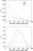 |
Fig. 10 πFn and Ps as functions of α for a model planet covered by ocean and with a center continent of sand between ±22° longitude and ±50° latitude (green, dashed-triple-dotted line). Also plotted: the functions for a homogeneous ocean planet (blue, dashed-dotted line), a homogeneous sand planet (orange, solid line) and a weighted sum of these with ~16% sand and ~84% ocean (gray, dashed line). |
Incidentally, for this planet, the flux and polarization signals calculated using the HI-code and the HH-code are virtually equal at α = 90°. At this phase angle, flux and polarization observations would thus not help to establish the existence of the continent. However, interpreting flux observations at smaller (larger) phase angles using the HH-code would result in an overestimation (underestimation) of the coverage with sand, while interpreting only polarization observations at smaller (larger) phase angles using the HH-code would result in an underestimation (overestimation) of the coverage with sand. The interpretation of the combined flux and polarization observations using the HH-code would fail and thus reveal that assuming a homogeneous mixture of sand and ocean pixels is not realistic.
4.2. Atmospheric inhomogeneities
The next model planet has a black surface, a gaseous atmosphere with optical thickness of 0.1 (no absorption), and a patchy cloud layer with an optical thickness of 2.0. The clouds are composed of liquid water particles described in size by the standard distribution of Hansen & Travis (1974), with an effective radius of 2.0 μm and an effective variance equal to 0.1 (model A particles of Karalidi et al. 2011). The single scattering albedo of our particles at 0.55 μm is 0.999534. For a detailed description of the single scattering properties of our cloud particles see Karalidi et al. (2011). The cloud layer is patchy (the clouds are composed of fully cloud covered pixels that cluster in random manner across the planetary surface) in the horizontal direction, but its vertical extension is the same all over the planet, namely from 3 km to 4 km in Earth’s atmosphere (279 K to 273 K).
Figure 11 shows πFn and P as functions of phase angle α of the model planet for different cloud coverages as calculated using the HI- and the HH-code. The flux phase functions for the different cloud coverages have different strengths, but very similar shapes. The phase functions as calculated using the HH-code have slightly sharper features near α = 0°. Note that the bump in the curves near α = 30° is the signature of the primary rainbow (see e.g. Karalidi et al. 2011): light that is scattered once by the cloud particles. As expected, the difference between the fluxes calculated with the two codes are small for small and large percentages of cloud coverage. For an intermediate, almost Earth-like, coverage of 42.3%, ΔπFn is as large as 15% at α = 0°. In this case, using the HH-code to interpret the flux reflected by the patchy cloudy planet near α = 0° would yield a cloud coverage of ~53%.
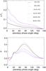 |
Fig. 11 πFn and Ps as functions of α for a model ocean planet with patchy clouds that cover 16%, 42.3%, or 83.9% of the planet. The curves as calculated using the HH-code and the weighted sum approximation are also shown. |
The polarization phase functions clearly show the different contributions of the light that is Rayleigh scattered by the gas molecules above and in particular between the patches of clouds (the strong values around α = 90°) and that of the light that is scattered by the cloud articles (the primary rainbow). Clearly, the larger the coverage of the clouds, the smaller the contribution of the purely Rayleigh scattered light to the total signal. Adding clouds to our model planet decreases the amount of purely Rayleigh scattered light, and thus decreases P around α = 90°. The strength of the primary rainbow in P is insensitive to the cloud coverage because adding clouds does not change the fraction of multiply scattered light within the clouds (the clouds have the same optical properties), which mostly determines the strength of the rainbow on these planets. The Rayleigh scattering polarization maximum around α = 90° does influence the contrast of the rainbow feature: for low cloud coverages it forms a shoulder on the Rayleigh scattering maximum, while for high coverages, it is a local maximum.
For small and large percentages of cloud coverage, the differences in the polarization phase functions due to using either the HI- or the HH-code are at most a few percent points around α = 90° (~−4% for 16%, and ~3% for 83.9% coverage). The differences are largest for the intermediate cloud coverage: about 10% for 42.3% coverage. In this case, using the HH-code to interpret the polarization reflected by the patchy cloudy planet near α = 90°, would yield a cloud coverage of ~25%. The degree of polarization calculated with the HI-code, and thus ΔP too, depends not only on the cloud coverage, but also on the locations of the clouds across the planet. Not surprisingly, this sensitivity is highest for intermediate cloud coverages.
4.3. Atmospheric and surface inhomogeneities
Finally, we present the flux and polarization signals of planets with patchy clouds (see Sect. 4.2), and a sandy continent in the middle of a black ocean (see Sect. 4.1). Figure 12 shows πFn and P as functions of α for 42.3% cloud coverage. The phase functions as calculated using the HH-code and the HI-code results for a cloudy planet without a continent are also shown.
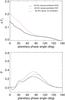 |
Fig. 12 πFn and Ps as functions of α for a model ocean planet with a central sandy continent and 42.3% cloud coverage as calculated using the HI-code (red, dashed line) and the HH-code and the weighted sum approximation (black, solid line). For comparison, the curves for a model ocean planet without the continent and with 42.3% cloud coverage are also shown (blue, dashed-dotted line). |
The continent strongly increases πFn. The increase will usually depend on the location of the clouds and the continent. In this case, the continent is located in the middle of the planetary disk, and thus has a large influence. Since only a small fraction (~8%) of the pixels on the disk contain sand, the flux calculated with the HH-code is only marginally higher than that calculated with the HH-code and without a continent (see Fig. 11). Inversely, if the HH-code would be used to interpret the flux signal of the cloudy planet with the continent, a 55% continental coverage and 24% clouds would be found.
The presence of the Lambertian reflecting continent below the clouds decreases the polarization phase function and shifts the maximum P towards larger α, when compared to the polarization phase function of the cloudy ocean planet. The primary rainbow is still visible in the phase function, albeit more like a shoulder than a local maximum.
Using polarimetry only, a straightforward fit to the polarization phase function with the HH-code would estimate the continental coverage at about 17% and the cloud coverage at 24%. When both πFn and P are taken into account the best fit is acquired for the case of 22% continental coverage and 19% cloud coverage.
5. Summary and conclusions
We have presented a numerical code that can be used to calculate disk integrated total and polarized fluxes of starlight that is reflected by horizontally inhomogeneous exoplanets, e.g. planets that are covered by oceans and continents, and/or overlaid by a patchy cloud deck.
For most types of model planets, our code for horizontally inhomogeneous planets (the HI-code) is computationally much more expensive than the code for horizontally homogeneous planets by Stam et al. (2006) combined with the so-called weighted sum approximation to simulate fluxes of horizontally inhomogeneous planets (the HH-code). In the latter method, total and polarized flux signals of different horizontally homogeneous planets are summed using weighting factors depending on which fraction of the illuminated and visible part of the horizontally inhomogeneous planet is represented by each type of planet. Only for planets with a large variation of horizontal inhomogeneities, such as a large number of different surface and cloud coverages, the computing time for the HH-code approaches that for the HI-code.
The main advantage of using the HI-code instead of the HH-code is obviously the ability to simulate signals of horizontally inhomogeneous planets. Other advantages of the HI-code are that since every pixel on the planet is treated separately, it allows taking into account effects of e.g. the non-sphericity of a planet, shadowing by planetary rings, and a spatial extension of the illuminating source.
Since for most model planets, our HI-code consumes much more computing time than the HH-code (Stam et al. 2006), it is interesting to investigate the influences of horizontal inhomogeneities on the total and polarized fluxes of starlight that is reflected by a planet. For three types of horizontally inhomogeneous planets covered by black and white surface pixels and overlaid by a gaseous atmosphere, we have calculated the fluxes and the degree of polarization as functions of the planetary phase angle α and compared them with results from the HH-code assuming the same percentage of black and white surface pixels and the same model atmosphere. Horizontal inhomogeneities can leave significant traces in both the reflected total flux πFn and the degree of linear polarization. However, while horizontal inhomogeneities appear to mostly influence the total amount of reflected flux and not so much the shape of the planet’s flux phase functions, they can strongly change the planet’s polarization phase functions in shape and strength. Indeed, fitting a planet’s polarization phase function using the HH-code would yield very different fractions of disk coverage (up to several tens of percent).
We also used the HI-code to calculate flux and polarization signals of Earth-like planets with surface and/or patchy clouds. These calculations confirmed that the shape of a planet’s flux phase function is fairly independent of the horizontal inhomogeneities. Obviously, the absolute values of the flux phase function does depend on the inhomogeneities, but it will also depend on the radius of the planet (in this paper we assumed a planetary radius equal to one), which thus would have to been known accurately to fit the flux phase function. The polarization phase function appears to be rather sensitive to the inhomogeneities, both its absolute values and the shape of the curve (e.g. location maximum value). Because the degree of polarization is a ratio, it is independent of the radius of a planet. The flux and polarization signals of planets are wavelength dependent (see e.g. Stam 2008), therefore the observability of horizontal inhomogeneities will also depend on the wavelength. In particular, at short wavelengths, the gas optical thickness is larger than at longer wavelengths, and will thus hamper the observations of the surface. Future studies could focus on which spectral bands should be combined to optimize retrieval schemes.
In the presence of liquid water clouds, the strength of the primary rainbow in the flux phase functions of Earth-like planets increases with increasing cloud coverage. Whether or not it would be detectable depends strongly on the sensitivity and stability of the observing instrument. In the polarization phase function, the strength of the rainbow is almost independent of the cloud coverage as long as the planet’s surface is very dark (i.e. does not add too much unpolarized flux to the total signal). A bright surface, such as a sandy continent, decreases the strength of the rainbow feature.
Properly accounting for horizontal inhomogeneities appears to significantly influence reflected fluxes and polarization signals, and should eventually be applied to interpret observations of horizontally inhomogeneous exoplanets or e.g. observations of Earth-shine (Sterzik et al. 2012). The HH-code (horizontally homogeneous planets combined with the weighted sum approximation), however, is still a strong tool for simulating signals to be used for the design and optimization of exoplanet observations, because its simulations cover the range of total and polarized fluxes that we can expect to observe. Because flux and polarization phase functions have different sensitivities to the inhomogeneities, a combination of flux and polarization observations would help to retrieve the actual planetary parameters.
Our results, and especially the differences between the fluxes and degrees of polarization of the reflected starlight, indicate which accuracies should be reached with flux and/or polarization observations in order to detect horizontal inhomogeneities on a planet. As such they can drive the design of instruments for exoplanet characterization. Assuming a super-Earth exoplanet (with a radius of 1.5 r⊕) orbiting a Sun-like star at 1 pc from the observer at a 40-m telescope (such as the E-ELT), a back-of-the-envelope calculation shows that a few nights of integration time (a total of 20 h) could yield an accuracy of 10-3. The phase angle of a planet in an Earth-like orbit would change by ~3° during that time. For this calculation we ignored the influence of stellar background light on the observation, and we didn’t include any actual instrument parameters, such as spectral bandwidths. Until results such as ours are combined with a realistic instrument and telescope simulator, the integration time estimate should thus be considered as a rough value.
References
- Beaulieu, J.-P., Bennett, D. P., Fouqué, P., et al. 2006, Nature, 439, 437 [NASA ADS] [CrossRef] [PubMed] [Google Scholar]
- Beaulieu, J. P., Kipping, D. M., Batista, V., et al. 2010, MNRAS, 409, 963 [NASA ADS] [CrossRef] [Google Scholar]
- Cash, W., & New Worlds Study Team 2010, in ASP Conf. Ser. 430, eds. V. Coudé Du Foresto, D. M. Gelino, & I. Ribas, 353 [Google Scholar]
- Charbonneau, D., Berta, Z. K., Irwin, J., et al. 2009, Nature, 462, 891 [NASA ADS] [CrossRef] [PubMed] [Google Scholar]
- de Haan, J. F., Bosma, P. B., & Hovenier, J. W. 1987, A&A, 183, 371 [NASA ADS] [Google Scholar]
- Ford, E. B., Seager, S., & Turner, E. L. 2001, Nature, 412, 885 [NASA ADS] [CrossRef] [PubMed] [Google Scholar]
- Hansen, J. E., & Hovenier, J. W. 1974, J. Atmos. Sci., 31, 1137 [NASA ADS] [CrossRef] [Google Scholar]
- Hansen, J. E., & Travis, L. D. 1974, Space Sci. Rev., 16, 527 [NASA ADS] [CrossRef] [Google Scholar]
- Hovenier, J. W., & van der Mee, C. V. M. 1983, A&A, 128, 1 [NASA ADS] [Google Scholar]
- Hovenier, J. W., Van der Mee, C., & Domke, H. 2004, Transfer of polarized light in planetary atmospheres: basic concepts and practical methods, Astrophys. Space Sci. Lib., 318 [Google Scholar]
- Kaltenegger, L., & Traub, W. A. 2009, ApJ, 698, 519 [NASA ADS] [CrossRef] [Google Scholar]
- Karalidi, T., Stam, D. M., & Hovenier, J. W. 2011, A&A, 530, A69 [NASA ADS] [CrossRef] [EDP Sciences] [Google Scholar]
- Keller, C. U., Schmid, H. M., Venema, L. B., et al. 2010, in SPIE Conf. Ser., 7735 [Google Scholar]
- Kemp, J. C., Henson, G. D., Steiner, C. T., & Powell, E. R. 1987, Nature, 326, 270 [NASA ADS] [CrossRef] [Google Scholar]
- Léger, A., Grasset, O., Fegley, B., et al. 2011, Icarus, 213, 1 [NASA ADS] [CrossRef] [Google Scholar]
- McClatchey, R. A., Fenn, R., Selby, J. E. A., Volz, F., & Garing, J. S. 1972, AFCRL-72.0497 (US Air Force Cambridge research Labs) [Google Scholar]
- Madhusudhan, N., & Burrows, A. 2012, ApJ, 747, 25 [NASA ADS] [CrossRef] [Google Scholar]
- Mayor, M., & Queloz, D. 1995, Nature, 378, 355 [NASA ADS] [CrossRef] [Google Scholar]
- Miller-Ricci, E., & Fortney, J. J. 2010, ApJ, 716, L74 [NASA ADS] [CrossRef] [Google Scholar]
- Mishchenko, M. I. 1990, Icarus, 84, 296 [NASA ADS] [CrossRef] [Google Scholar]
- Oakley, P. H. H., & Cash, W. 2009, ApJ, 700, 1428 [NASA ADS] [CrossRef] [Google Scholar]
- Press, W. H., Teukolsky, S. A., Vetterling, W. T., & Flannery, B. P. 1992, Numerical recipes in FORTRAN, The art of scientific computing, eds. W. H. Press, S. A. Teukolsky, W. T. Vetterling, & B. P. Flannery [Google Scholar]
- Saar, S. H., & Seager, S. 2003, in Scientific Frontiers in Research on Extrasolar Planets, eds. D. Deming, & S. Seager, ASP Conf. Ser., 294, 529 [Google Scholar]
- Seager, S., Whitney, B. A., & Sasselov, D. D. 2000, ApJ, 540, 504 [NASA ADS] [CrossRef] [Google Scholar]
- Stam, D. M. 2003, in Earths: DARWIN/TPF and the Search for Extrasolar Terrestrial Planets, eds. M. Fridlund, T. Henning, & H. Lacoste, ESA Spec. Publ., 539, 615 [Google Scholar]
- Stam, D. M., de Rooij, W. A., Cornet, G., & Hovenier, J. W. 2006, A&A, 452, 669 [NASA ADS] [CrossRef] [EDP Sciences] [MathSciNet] [Google Scholar]
- Stam, D. M., & Hovenier, J. W. 2005, A&A, 444, 275 [NASA ADS] [CrossRef] [EDP Sciences] [Google Scholar]
- Stam, D. M., Hovenier, J. W., & Waters, L. B. F. M. 2004, A&A, 428, 663 [NASA ADS] [CrossRef] [EDP Sciences] [Google Scholar]
- Stam, D. M. 2008, A&A, 482, 989 [NASA ADS] [CrossRef] [EDP Sciences] [Google Scholar]
- Sterzik, M. F., Bagnulo, S., & Palle, E. 2012, Nature, 483, 64 [NASA ADS] [CrossRef] [Google Scholar]
- Tinetti, G., Meadows, V. S., Crisp, D., et al. 2006, Astrobiology, 6, 881 [NASA ADS] [CrossRef] [PubMed] [Google Scholar]
- Tomasko, M. G., Doose, L. R., Dafoe, L. E., & See, C. 2009, Icarus, 204, 271 [NASA ADS] [CrossRef] [Google Scholar]
- Zugger, M. E., Kasting, J. F., Williams, D. M., Kane, T. J., & Philbrick, C. R. 2010, ApJ, 723, 1168 [NASA ADS] [CrossRef] [Google Scholar]
Appendix A: Testing our numerical code
Here, we present the results of testing our numerical code for horizontally inhomogeneous planets (from hereon the HI-code). We have tested our code by comparing it to results of the code for horizontally homogeneous planets Stam et al. (2006) (from hereon the HH-code).
A.1. Horizontally homogeneous planets
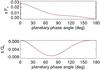 |
Fig. A.1 Normalised reflected fluxes πFn and πQn as functions of the planetary phase angle α for a black planet with a gaseous atmosphere as calculated using the HH-code (solid lines) and the HI-code (dashed lines). The solid and dashed lines coincide. |
For the first comparison between our HI-code and the HH-code, we used both codes to calculate the light reflected by a model planet with a black surface and a gaseous, Rayleigh scattering atmosphere with a total optical thickness of about 0.1. For the HI-code, the planet was divided into pixels of 2° × 2° (latitude × longitude).
Figure A.1 shows the excellent agreement between the reflected fluxes πFn and πQn as functions of phase angle α calculated using the two codes (because the planet is mirror-symmetric with respect to the reference plane, πUn = 0). The absolute difference between the fluxes calculated by the two codes is smaller than 10-5. Figure A.2 shows the degree of polarization Ps (= −Q/F) (see Eq. (3)) calculated using both codes, and the absolute difference ΔPs between the curves. ΔPs is largest around small (15°) and large (160°) phase angles, which is due to the size of the pixels. Since in the HI-code, we use one set of angles θ0, θ, Δφ, and β2 for each pixel, the larger a pixel, the less this set of angles represents the range of angles across the pixel. The error is largest for pixels along the planetary limb and terminator, and thus for the large and small phase angles (at the small angles, the degree of polarization in the centre of the disk is close to zero, making the contribution of the limb pixels thus significant). At α = 0° and 180°, Ps of the planet is zero and thus ΔPs, too.
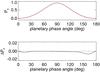 |
Fig. A.2 The degree of polarization Ps corresponding to the fluxes shown in Fig. A.1 (the two lines coincide) and the absolute difference between the two lines. |
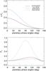 |
Fig. A.3 πFn and Ps as functions of α for a black planet (gray, dashed-triple-dotted line), a white planet (blue, dashed-dotted line), and a planet with a gaseous atmosphere and its surface overed by alternating black and white pixels (black, solid line). The latter curves coincide with those calculated using horizontally homogeneous planets and a weighted sum approximation (red, dashed line). All planets are cloud-free. |
For a model planet with a gaseous atmosphere, the differences between the results of the two codes appear to be fairly independent of the albedo of a (Lambertian reflecting) surface: with a white surface, the absolute differences in πFn and πQn, and ΔPs are similar to those with a black surface. For a model planet with a horizontally homogeneous cloud layer of optical thickness 1, composed of the model A cloud particles of Karalidi et al. (2011), and a surface albedo of 0.1, the absolute difference in the fluxes increased slightly to a maximum value of 5 × 10⁻⁵ and the maximum ΔPs increased to ~0.0062. These differences didn’t change significantly when other (e.g. larger) cloud particles were used.
The comparison with the HH-code shows that the integration across the disk by our HI-code is accurate enough for application to horizontally homogeneous planets, provided small enough pixels are used across the disk.
A.2. Horizontally inhomogeneous planets
For a second test of our HI-code, we used model planets with surfaces covered by two types of 2° × 2° pixels that alternate in longitude and latitude (they thus look like chess boards). The equator of each planet coincides with the planetary scattering plane. The planetary atmospheres are gaseous, Rayleigh scattering and have an optical thickness of 0.1. While our HI-code can handle these types of planets, the HH-code cannot. Therefore, as in Stam (2008), weighted sums of flux vectors reflected by horizontally homogeneous planets are used to approximate the flux vectors of horizontally inhomogeneous planets. The flux vector of a planet covered by J different types of pixels (with a different atmosphere and/or surface) is thus calculated using  (A.1)with πFj the flux vector of starlight reflected by a planet that is completely covered by type j pixels, and with wj the fraction of type j pixels on the horizontally inhomogeneous planet.
Figure A.3 shows πFn and Ps as functions of phase angle α for a planet with its surface covered by alternating black and Lambertian reflecting white pixels as calculated with the HI-code and the HH-code (the latter combined with the weighted sum approximation, see Eq. (A.1)). For comparison, πFn and Ps are also shown for horizontally homogeneous black and white planets.
The absolute difference between the fluxes of starlight reflected by the black-and-white planet as calculated using the HI-code and the HH-code is smaller than 7 × 10⁻⁵, and between
the degrees of polarization smaller than 0.005 across the whole phase angle range. It appears that the differences between the results of the two codes depend slightly on the surface albedo: decreasing the albedo of pixels from 1.0 to 0.24 (which is typical for a sand surface at 0.55 μm), the difference in the flux decreases to 5 × 10⁻⁵ and in the polarization to 0.004.
The comparison with the HH-code applied to horizontally homogeneous planets and using the weighted sum approximation shows that our HI-code is accurate enough for application to horizontally inhomogeneous planets, provided enough pixels are used across the disk.
All Figures
|
Fig. 1 πFn and Ps as functions of α for black, cloud-free planets with white spots occupying 4% (red, dotted line), 21% (green, dashed line), 41% (blue, dashed-dotted line), 57% (grey, dashed-triple-dotted line) and 68% (purple, long-dashed line) of the planet. |
| In the text | |
|
Fig. 2 Relative difference ΔπFn and the absolute difference ΔPs between the flux and polarization phase functions of the white spotted planets of Fig. 1 as calculated using the HI-code and the HH-code. The coverage of white spots is 4% (red, dotted line), 21% (green, dashed line), 41% (blue, dashed-dotted line), 57% (grey, dashed-tripple-dotted line) and 68% (purple, long-dashed line). |
| In the text | |
|
Fig. 3 πFn and Ps as functions of α for black, cloud-free planets with a white continent on the center of the planetary disk facing the observer, for different coverages of the continent: 5% (black, solid line), 12% (red, dashed line), 21% (blue, dashed-dotted line), 32% (green, dashed-triple-dotted line), 80% (magenta, long-dashed line) and 98% (gray, dotted line). |
| In the text | |
|
Fig. 4 ΔπFn and ΔPs between the phase functions of the white continent planets of Fig. 3 as calculated using the HI-code and the HH-code. The coverage of the continents is: 5% (black, solid line), 12% (red, dashed line), 21% (blue, dashed-dotted line), 32% (green, dashed-triple-dotted line), 80% (magenta, long-dashed line) and 98% (gray, dotted line) of the planetary disk. |
| In the text | |
|
Fig. 5 Similar to Fig. 4, except for white, cloud-free planets with black continents. The coverage of the continents is: 5% (black, solid line), 21% (red, dashed line), 46% (blue, dashed-dotted line), and 80% (green, dashed-triple-dotted line) of the planetary disk. |
| In the text | |
|
Fig. 6 πFn and P as functions of α for black, cloud-free planets with hemispherical caps occupying 23% (black, solid line), 43% (red, dashed line), 61% (blue, dashed-dotted line), and 77% (green, dashed-triple-dotted line) of the planet. The caps are located at the “north” and “south” poles of the planet. |
| In the text | |
|
Fig. 7 ΔπFn and ΔPs between the phase functions of the capped planets of Fig. 6 as calculated using the HI-code and the HH-code. The caps occupy 23% (black, solid line), 43% (red, dashed line), 61% (blue, dashed-dotted line) and 77% (green, dashed-triple-dotted line) of the planet. |
| In the text | |
|
Fig. 8 πFn and P as functions of α for black, cloud-free planets with white, hemispherical caps that occupy 23% of the planet. The locations of the caps are: 0° (black, solid line), indicating the caps are on the “north” and “south” poles of the planet, 45° (red, dashed line), and 90° (blue, dashed-dotted line), with the caps on the “eastern” and “western” sides of the planetary disk. |
| In the text | |
|
Fig. 9 ΔπFn and ΔPs between the phase functions of the capped planets of Fig. 8 as calculated using the HI-code and the HH-code. The cap locations are: 0° (black, solid line), 45° (red, dashed line), and 90° (blue, dashed-dotted line). |
| In the text | |
|
Fig. 10 πFn and Ps as functions of α for a model planet covered by ocean and with a center continent of sand between ±22° longitude and ±50° latitude (green, dashed-triple-dotted line). Also plotted: the functions for a homogeneous ocean planet (blue, dashed-dotted line), a homogeneous sand planet (orange, solid line) and a weighted sum of these with ~16% sand and ~84% ocean (gray, dashed line). |
| In the text | |
|
Fig. 11 πFn and Ps as functions of α for a model ocean planet with patchy clouds that cover 16%, 42.3%, or 83.9% of the planet. The curves as calculated using the HH-code and the weighted sum approximation are also shown. |
| In the text | |
|
Fig. 12 πFn and Ps as functions of α for a model ocean planet with a central sandy continent and 42.3% cloud coverage as calculated using the HI-code (red, dashed line) and the HH-code and the weighted sum approximation (black, solid line). For comparison, the curves for a model ocean planet without the continent and with 42.3% cloud coverage are also shown (blue, dashed-dotted line). |
| In the text | |
|
Fig. A.1 Normalised reflected fluxes πFn and πQn as functions of the planetary phase angle α for a black planet with a gaseous atmosphere as calculated using the HH-code (solid lines) and the HI-code (dashed lines). The solid and dashed lines coincide. |
| In the text | |
|
Fig. A.2 The degree of polarization Ps corresponding to the fluxes shown in Fig. A.1 (the two lines coincide) and the absolute difference between the two lines. |
| In the text | |
|
Fig. A.3 πFn and Ps as functions of α for a black planet (gray, dashed-triple-dotted line), a white planet (blue, dashed-dotted line), and a planet with a gaseous atmosphere and its surface overed by alternating black and white pixels (black, solid line). The latter curves coincide with those calculated using horizontally homogeneous planets and a weighted sum approximation (red, dashed line). All planets are cloud-free. |
| In the text | |
Current usage metrics show cumulative count of Article Views (full-text article views including HTML views, PDF and ePub downloads, according to the available data) and Abstracts Views on Vision4Press platform.
Data correspond to usage on the plateform after 2015. The current usage metrics is available 48-96 hours after online publication and is updated daily on week days.
Initial download of the metrics may take a while.