| Issue |
A&A
Volume 545, September 2012
|
|
|---|---|---|
| Article Number | A79 | |
| Number of page(s) | 19 | |
| Section | Numerical methods and codes | |
| DOI | https://doi.org/10.1051/0004-6361/201219074 | |
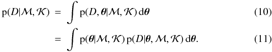
| Published online | 11 September 2012 | |
Bayesian analysis of exoplanet and binary orbits⋆
Demonstrated using astrometric and radial-velocity data of Mizar A
Max-Planck-Institut für Astronomie, Königstuhl 17, 69117
Heidelberg,
Germany
e-mail: This email address is being protected from spambots. You need JavaScript enabled to view it.
Received:
20
February
2012
Accepted:
12
July
2012
Abstract
Aims. We introduce BASE (Bayesian astrometric and spectroscopic exoplanet detection and characterisation tool), a novel program for the combined or separate Bayesian analysis of astrometric and radial-velocity measurements of potential exoplanet hosts and binary stars. The capabilities of BASE are demonstrated using all publicly available data of the binary Mizar A.
Methods. With the Bayesian approach to data analysis we can incorporate prior knowledge and draw extensive posterior inferences about model parameters and derived quantities. This was implemented in BASE by Markov chain Monte Carlo (MCMC) sampling, using a combination of the Metropolis-Hastings, hit-and-run, and parallel-tempering algorithms to explore the whole parameter space. Nonconvergence to the posterior was tested by means of the Gelman-Rubin statistic (potential scale reduction). The samples were used directly and transformed into marginal densities by means of kernel density estimation, a “smooth” alternative to histograms. We derived the relevant observable models from Newton’s law of gravitation, showing that the motion of Earth and the target can be neglected.
Results. With our methods we can provide more detailed information about the parameters than a frequentist analysis does. Still, a comparison with the Mizar A literature shows that both approaches are compatible within the uncertainties.
Conclusions. We show that the Bayesian approach to inference has been implemented successfully in BASE, a flexible tool for analysing astrometric and radial-velocity data.
Key words: astrometry / celestial mechanics / methods: data analysis / methods: statistical / techniques: interferometric / techniques: radial velocities
BASE, the computer program introduced in this article, can be downloaded at http://www.mpia.de/homes/schulze/base.html.
© ESO, 2012
1. Introduction
The search for extrasolar planets – places where one day humankind might find other forms of life in the Universe – has been a subject of scientific investigation since the nineteenth century, but only became successful in 1992 with the first confirmed discovery of an exoplanet orbiting the pulsar PSR B1257+12 (Wolszczan & Frail 1992). Still, because it is situated in an environment hostile to life as we know it, this case has been of less relevance to the public than the first detection of a Sun-like planet-host star, 51 Pegasi (Mayor & Queloz 1995). Since that time, more than 700 extrasolar planet candidates have been unveiled in more than 500 systems, more than 90 of which show signs of multiplicity (Schneider 2012).
Closely related to the detection of extrasolar planets is the characterisation of their orbits. Both these tasks now profit from the existence of a variety of observational techniques, which we briefly sketch in the following. Comprehensive reviews can be found in Perryman (2000) and Deeg et al. (2007).
Direct observational methods refer to the imaging of exoplanets (e.g. Levine et al. 2009), which reflect the light of their host stars but also emit their own thermal radiation. To overcome the major obstacle of the high brightness contrast between planet and star, techniques such as coronagraphy (Lyot 1932; Levine et al. 2009), angular differential imaging (Marois et al. 2006; Vigan et al. 2010), spectral differential imaging (Smith 1987; Vigan et al. 2010), and polarimetric differential imaging (Kuhn et al. 2001; Adamson et al. 2005) have been invented. Still, imaging has only revealed few detections and orbit determinations so far.
The most productive methods in terms of the number of detected and characterised exoplanets are of an indirect nature, observing the effects of the planet on other objects or their radiation.
Of these, transit photometry (e.g. Charbonneau et al. 2000; Seager 2008) is noteworthy because it has helped uncover more than 200 exoplanet candidates, plus over 2000 still unconfirmed candidates from the Kepler space mission (Koch et al. 2010): small decreases in the apparent visual brightness of a star during the primary or secondary eclipse point to the existence of a transiting companion. These data allow one to determine the planet’s radius and orbital inclination and may also yield information on the planet’s own radiation.
Timing methods include measurements of transit timing variations (TTV) and transit duration variations (TDV) (e.g. Holman & Murray 2005; Nascimbeni et al. 2011) of either binaries or stars known to harbour a transiting planet. The method used in the first exoplanet detection (Wolszczan & Frail 1992) is pulsar timing, which relies on slight anomalies in the exact timing of the radio emission of a pulsar and is sensitive to planets in the Earth-mass regime.
Microlensing (Mao & Paczynski 1991; Gould 2009), which accounted for about 15 exoplanet candidates, uses the relativistic curvature of spacetime due to the masses of both a lens star and its potential companion, with the latter causing a change in the apparent magnification and thus the observed brightness of a background source.
Perhaps the most well-known technique, and one of those on which this article is based, is
known as Doppler spectroscopy or radial-velocity (RV) measurements (e.g. Mayor & Queloz 1995; Lovis & Fischer 2010). With more than 500 exoplanet candidates, it has been
most successful in detecting new exoplanets and determining their orbits to date. From a set
of high-resolution spectra of the target star, a time series of the line-of-sight velocity
component of the star is deduced. These data allow one to determine the orbit in terms of
its geometry and kinematics in the orbital plane as well as the minimum planet
mass mp,min ≈ mpsini.
To derive the actual planet mass mp, the
inclination i of the orbit plane with respect to the sky plane needs to
be derived with a different method, e.g. astrometry. The RV technique is
distance-independent by principle, but signal-to-noise requirements do pose constraints on
the maximum distance to a star. Stellar variability sometimes makes this approach difficult
because it alters the line shapes and thus mimicks RV variations. The signal in stellar RVs
caused by a planet in a circular orbit has a semi-amplitude of approximately 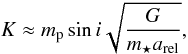 (1)where
mp,m⋆,i,G,
and arel are the masses of planet and host star, the orbital
inclination, Newton’s gravitational constant, and the semi-major axis of the planet’s orbit
relative to the star, respectively. This approximation holds for
mp ≪ m⋆, which
is true in most cases. It should be noted that the sensitivity of the RV method decreases
towards less inclined (more face-on) orbits, which is an example for the selection effects
inherent to any planet-detection method.
(1)where
mp,m⋆,i,G,
and arel are the masses of planet and host star, the orbital
inclination, Newton’s gravitational constant, and the semi-major axis of the planet’s orbit
relative to the star, respectively. This approximation holds for
mp ≪ m⋆, which
is true in most cases. It should be noted that the sensitivity of the RV method decreases
towards less inclined (more face-on) orbits, which is an example for the selection effects
inherent to any planet-detection method.
Finally, astrometry (AM; e.g. Gatewood et al. 1980;
Sozzetti 2005; Reffert 2009) – on which this work is also based – is the oldest observational
technique known in astronomy: a stellar position is measured with reference to a given point
and direction on sky. Astrometry can thus be considered as complementary to Doppler
spectroscopy, which measures the kinematics perpendicular to the sky plane. In contrast to
the latter, AM allows one to determine the orientation of the orbital plane relative to the
sky in terms of its inclination i and the position angle Ω of the line of
nodes with respect to the meridian of the target. A planet in circular orbit around its host
star displaces the latter on sky with an approximate angular semi-amplitude of 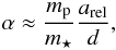 (2)where d is the distance
between the star and the observer. Again, this approximation holds for
mp ≪ m⋆.
(2)where d is the distance
between the star and the observer. Again, this approximation holds for
mp ≪ m⋆.
Imaging astrometry, in its attempt to reach sufficient presicion, still faces problems due to various distortion effects. By contrast, interferometric astrometry has been used to determine the orbits of previously known exoplanets, mainly with the help of space-borne telescopes such as Hipparcos or the Hubble Space Telescope (HST), which presently still excel their Earth-bound competitors (e.g. McArthur et al. 2010). However, instruments like PRIMA (Delplancke et al. 2000; Delplancke 2008; Launhardt et al. 2008) or GRAVITY (Gillessen et al. 2010) at the ESO Very Large Telescope Interferometer are promising to advance ground-based AM even more in the near future.
While planet-induced signals in AM and RVs are both approximately linear in planetary mass mp, they differ in their dependence on the orbital semi-major axis arel (Eqs. (1) and (2)). Doppler spectroscopy is more sensitive to smaller orbits (or higher orbital frequencies, Eq. (45)), while AM favours larger orbital separations, viz. longer periods.
In this article we introduce BASE, a Bayesian astrometric and spectroscopic exoplanet detection and characterisation tool. Its goals are to fulfil two major tasks of exoplanet science, namely the detection of exoplanets and the characterisation of their orbits. BASE has been developed to provide for the first time the possibility of an integrated Bayesian analysis of stellar astrometric and Doppler-spectroscopic measurements with respect to their companions’ signals1, correctly treating the measurement uncertainties and allowing one to explore the whole parameter space without the need for informative prior constraints. Still, users may readily incorporate prior knowledge, e.g. from previous analyses with other tools, by means of priors on the model parameters. The tool automatically diagnoses convergence of its Markov chain Monte Carlo (MCMC) sampler to the posterior and regularly outputs status information. For orbit characterisation, BASE delivers important results such as the probability densities and correlations of model parameters and derived quantities.
Because published high-precision AM observations of potential exoplanet host stars are still sparse, we used data of the well-known binary Mizar A to demonstrate the capabilities of BASE. It is also planned to gain astrophysical insights into exoplanet systems using BASE in the near future.
This article is organised as follows. Section 2 provides an overview of the most often-used methods of data analysis, including Bayes’ theorem and MCMC as theoretical and implementational foundations of this work, as well as a derivation of the necessary observable models. BASE is described in Sect. 3. In Sect. 4, the target Mizar A and the data used in this article are discussed. Section 5 presents and discusses our analysis of Mizar A. Conclusions are drawn in Sect. 6.
2. Methods and models
Data analysis is a type of inductive reasoning in that it infers general rules from specific observational data (e.g. Gregory 2005b). These general rules are described by observable models, simply called models in the following, which produce theoretical values of the observables as a function of parameters. The primary tasks of data analysis are listed in the following.
-
1.
In model selection, the relative probabilities of a set ofconcurrent models {ℳi}, chosen a priori, are assessed. Specifically, exoplanet detection tries to decide the question of whether a certain star is accompanied by a planet or not, based on available data. Additionally, model-assessment techniques can be used to determine whether the most probable model describes the data accurately enough.
-
2.
Parameter estimation aims to determine the parameters θ of a chosen model. This is specifically referred to as exoplanet characterisation (or orbit determination) in the present context.
-
3.
The purpose of uncertainty estimation is to provide a measure of the parameters’ uncertainties.
Although model selection is equally important, in what follows we focus entirely on the second and third tasks, viz. parameter and uncertainty estimation. This is because for a known binary system, only one model is appropriate, viz. two bodies orbiting each other. Accordingly, BASE can only perform model selection when it analyses data from stars for which it is a-priori unknown whether a companion exists.
2.1. Likelihoods and frequentist inference
The well-established, conventional frequentist approach to inference is touched upon only briefly here. Its name stems from the fact that it defines probability as the relative frequency of an event. Measurements are regarded as values of random variables drawn from an underlying population that is characterised by population parameters, e.g. mean and standard deviation in the case of a normal (Gaussian) population. In the following, we derive the joint probability density of the values of AM and RV data, known as the likelihood ℒ, which plays a central role in frequentist inference.
When combining data of different types, one should generally be aware that potential systematic errors may differ between the data sets, e.g. due to a calibration error in one instrument that renders the data inconsistent with each other. In this case, each data set analysed separately would imply a different result. In other instances, systematic errors in one set do not affect the other data: for example, any constant offset in radial velocity is absorbed into parameter V, which is irrelevant to the analysis of astrometric data. In the following derivation, we assumed that no systematic effects are present that led to inconsistent data.
In the following, we assumed that the error ϵi of any datum yi is statistically independent of those of all other data and consists of two components, each distributed according to a (uni- or bivariate) normal distribution with zero mean:
-
a component ϵ0,i corresponding to a nominal measurement error, whose distribution is characterised by the covariance matrix E0,i or standard deviation σ0,i given with the datum, for AM and RV data respectively, and
-
a component ϵ + ,i representing e.g. instrumental, atmospheric or stellar effects not modelled otherwise, whose distribution is characterised by scalar covariance matrix
 – assuming no correlation between
the noise in the two AM components – or
variance
– assuming no correlation between
the noise in the two AM components – or
variance  , respectively, where
τ+ and σ+ are free
noise-model parameters.
, respectively, where
τ+ and σ+ are free
noise-model parameters.
The AM data covariance matrix E0,i of
datum i, representing the uncertainty of and correlation between the
two components measured, can be written using singular-value decomposition as
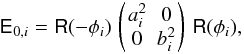 (3)where
R(·),ai,bi
and φi are the 2 × 2 passive rotation matrix,
the nominal semi-major and -minor axes of the uncertainty ellipse and the position angle
of its major axis, respectively.
(3)where
R(·),ai,bi
and φi are the 2 × 2 passive rotation matrix,
the nominal semi-major and -minor axes of the uncertainty ellipse and the position angle
of its major axis, respectively.
Using characteristic functions, it is readily shown that the sum ϵi = ϵ0,i + ϵ + ,i of the two independent error components is again normally distributed, with zero mean and covariance matrix Ei = E0,i + E+ or standard deviation , respectively.
The probability density2 of the values of
NAM two-dimensional AM
data  and NRV RV
data {vi}, known as the likelihood ℒ, is
then given by
and NRV RV
data {vi}, known as the likelihood ℒ, is
then given by 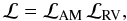 (4)where ℒAM and ℒRV are
the likelihoods pertaining to the individual data types,
(4)where ℒAM and ℒRV are
the likelihoods pertaining to the individual data types,
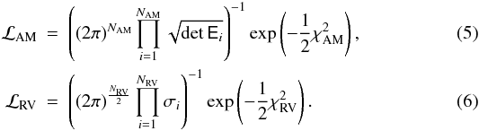 Furthermore, the sums of squares
 and
and
 are defined by
 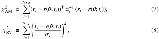 where
ri,vi
are the ith AM and RV datum,
r(·;·),v(·;·) the AM and RV model
functions and θ is the vector of model parameters. The
relevant models are derived in Sect. 2.3.
where
ri,vi
are the ith AM and RV datum,
r(·;·),v(·;·) the AM and RV model
functions and θ is the vector of model parameters. The
relevant models are derived in Sect. 2.3.
Parameter estimation.
Frequentist parameter estimation is generally equivalent to maximising ℒ or minimising
χ2 as functions of θ. The
resulting best estimates of the parameters  are therefore often called maximum-likelihood or least-squares estimates. For linear
models, χ2(θ) is a quadratic
function and consequently
can be found unambiguously by matrix inversion. In the more realistic cases of nonlinear
models, however, χ2 may have many local minima, therefore
care needs to be taken not to mistake a local minimum for the global one. Several
methods exist to this end, including evaluation of
χ2(θ) on a finite grid,
simulated annealing or genetic algorithms (e.g. Gregory
2005b).
are therefore often called maximum-likelihood or least-squares estimates. For linear
models, χ2(θ) is a quadratic
function and consequently
can be found unambiguously by matrix inversion. In the more realistic cases of nonlinear
models, however, χ2 may have many local minima, therefore
care needs to be taken not to mistake a local minimum for the global one. Several
methods exist to this end, including evaluation of
χ2(θ) on a finite grid,
simulated annealing or genetic algorithms (e.g. Gregory
2005b).
Uncertainty estimation.
Frequentist parameter uncertainties are usually quoted as confidence intervals. Procedures to derive these are designed such that when repeated many times based on different data, a certain fraction of the resulting intervals will contain the true parameters. Popular methods use bootstrapping (Efron & Tibshirani 1993) or the Fischer information matrix, which is based on a local linearisation of the model (e.g. Ford 2004). However, these methods suffer from specific caveats: the Fischer matrix is only appropriate for a quadratic-shaped χ2 in the vicinity of the minimum, and bootstrapping, which relies on modified data, may lead to severe misestimation of the parameter uncertainties, especially when these are large (Vogt et al. 2005).
2.2. Bayesian inference
Bayesian inference (e.g. Sivia 2006), which has
gained popularity in various scientific disciplines during the past few decades, defines
probability as the degree of belief in a certain hypothesis ℋ. While this is sometimes
criticised as leading to subjective assignments of probabilities, Bayesian probabilities
are not subjective if they are based on all relevant
knowledge  ,
hence different people having the same knowledge will assign them the same value (e.g.
Sivia 2006). Thus, Bayesian probabilities are
conditional on the knowledge ,
and this conditionality should be stated explicitly, as in the following equations.
,
hence different people having the same knowledge will assign them the same value (e.g.
Sivia 2006). Thus, Bayesian probabilities are
conditional on the knowledge ,
and this conditionality should be stated explicitly, as in the following equations.
2.2.1. Bayes’ theorem
In the eighteenth century, Thomas Bayes laid the foundation of a new approach to
inference with what is now known as Bayes’ theorem (Bayes
& Price 1763). For the purpose of parameter and uncertainty estimation, the
hypothesis ℋ refers to the values of model parameters θ,
and Bayes’ theorem can be expressed as  (9)where p(·) is a probability (density).
Furthermore,
D ≡ {(ti,yi)}
is the set of pairs of observational times3 and
corresponding data values, and ℳ denotes the particular model assumed. As mentioned
above, all probabilities are also conditional on the
knowledge ,
including statements on the types of parameters and the parameter space Θ (which we
assume to be a subset of Rk with k ∈ N) as
well as the noise model.
(9)where p(·) is a probability (density).
Furthermore,
D ≡ {(ti,yi)}
is the set of pairs of observational times3 and
corresponding data values, and ℳ denotes the particular model assumed. As mentioned
above, all probabilities are also conditional on the
knowledge ,
including statements on the types of parameters and the parameter space Θ (which we
assume to be a subset of Rk with k ∈ N) as
well as the noise model.
Using Bayes’ theorem, the aim is to determine the posterior
 ,
i.e. the probability distribution of the parameters θ in
light of the data D, given the model ℳ and prior
knowledge .
The other terms, located on the right-hand side of the theorem, are explained below.
,
i.e. the probability distribution of the parameters θ in
light of the data D, given the model ℳ and prior
knowledge .
The other terms, located on the right-hand side of the theorem, are explained below.
-
The term prior refers to the probability distribution
 of the parameters θ given only the model and prior
knowledge ;
it characterises the knowledge about the parameters present before considering the
data. For objective choices of priors, based on classes of parameters, see
Sect. A.
of the parameters θ given only the model and prior
knowledge ;
it characterises the knowledge about the parameters present before considering the
data. For objective choices of priors, based on classes of parameters, see
Sect. A. -
The likelihood
 is the probability distribution of the data values D, given the
times of observation, the model and the parameters. It is introduced in the
context of frequentist inference in Sect. 2.1.
is the probability distribution of the data values D, given the
times of observation, the model and the parameters. It is introduced in the
context of frequentist inference in Sect. 2.1. -
The evidence is the probability distribution of the data values D, given the times of observation and the model but neglecting the parameter values,
 It equals the integral of the product
of prior and likelihood over the parameter space Θ and plays the role of a
normalising constant, which is hard to calculate in practice, however.
It equals the integral of the product
of prior and likelihood over the parameter space Θ and plays the role of a
normalising constant, which is hard to calculate in practice, however.
It may be instructive here to note that the frequentist approach of maximising the
likelihood
is equivalent to maximising the posterior when assuming uniform
priors .
This can be seen by inserting  into Eq. (9), which leads to
 (12)However, this maximum-likelihood approach
ignores the fact that uniform priors are not always the most objective choice (see
Appendix A) and the posterior cannot be fully
characterised just by the position of its maximum. Still, the latter can be used as a
posterior summary in the Bayesian framework (Sect. 2.2.2).
(12)However, this maximum-likelihood approach
ignores the fact that uniform priors are not always the most objective choice (see
Appendix A) and the posterior cannot be fully
characterised just by the position of its maximum. Still, the latter can be used as a
posterior summary in the Bayesian framework (Sect. 2.2.2).
2.2.2. Posterior inference
Sampling from the posterior.
To estimate the normalised posterior  ,
i.e. the probability distribution of the parameters θ in
light of the data, N samples of the parameter vector
,
i.e. the probability distribution of the parameters θ in
light of the data, N samples of the parameter vector
 are collected using the Markov chain
Monte Carlo method (MCMC; e.g. Gilks et al.
1996) in the variant described by the Metropolis-Hastings algorithm (MH;
Metropolis et al. 1953; Hastings 1970), which performs a random walk through parameter
space. The distribution of these samples – excluding the first
M < N burn-in samples, which are still strongly
correlated with the starting state θ(0) –
converges to the posterior
are collected using the Markov chain
Monte Carlo method (MCMC; e.g. Gilks et al.
1996) in the variant described by the Metropolis-Hastings algorithm (MH;
Metropolis et al. 1953; Hastings 1970), which performs a random walk through parameter
space. The distribution of these samples – excluding the first
M < N burn-in samples, which are still strongly
correlated with the starting state θ(0) –
converges to the posterior  in the limit of many samples if the chain obeys certain regularity conditions (e.g.
Roberts 1996). Methods for setting the
starting state θ(0) and detecting convergence
are described in Sect. 3.4.
in the limit of many samples if the chain obeys certain regularity conditions (e.g.
Roberts 1996). Methods for setting the
starting state θ(0) and detecting convergence
are described in Sect. 3.4.
Starting from the current chain link θ(j + 1) ∈ Θ, the following steps lead to the next link, according to the MH algorithm and the hit-and-run sampler (step 1; Boneh & Golan 1979; Smith 1980):
-
1.
Set up a candidate C:
-
(a)
sample a direction, viz. a random unit vector d ∈ Rk from an isotropic density over the k-dimensional unit sphere;
-
(b)
sample a (signed) distance r from a uniform distribution over the interval { r′ ∈ R:θ(j) + r′d ∈ Θ } ;
-
(c)
set candidate C ≡ θ(j) + rd;
-
(a)
-
2.
calculate the acceptance probability
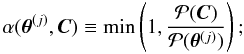 (13)
(13) -
3.
draw a random number β from a uniform distribution over the interval [0,1] ;
-
4.
if β ≤ α, accept the candidate, i.e. set the next link θ(j + 1) ≡ C; otherwise, θ(j + 1) ≡ θ(j).
The hit-and-run sampler, compared to alternatives like the Gibbs sampler (Geman & Geman 1984), favours exploring of the whole parameter space Θ without becoming “trapped” in the vicinity of a local posterior maximum (Gilks et al. 1996).
Because only the ratio of two posterior values is used (step 2), the normalising
evidence  – a constant that is difficult to determine, as mentioned above – is irrelevant in the
MH algorithm.
– a constant that is difficult to determine, as mentioned above – is irrelevant in the
MH algorithm.
Marginalisation and density estimation.
Obviously, the posterior mode alone reveals only one particular aspect of the posterior. However, as a density over k > 2 dimensions, the posterior cannot be displayed unambiguously in a figure.
To obtain a plottable summary of the posterior, a set of marginal
posteriors  ,
i.e. probability densities over each of the
parameters θi, and joint marginal
posteriors
,
i.e. probability densities over each of the
parameters θi, and joint marginal
posteriors  over two parameters, can be estimated. Theoretically, these densities are derived from
the posterior density by marginalisation, viz. integration over all other parameters,
over two parameters, can be estimated. Theoretically, these densities are derived from
the posterior density by marginalisation, viz. integration over all other parameters,
 where
where
 and
and  .
Practically, marginal posteriors are estimated by only considering
component i of the collected
samples
.
Practically, marginal posteriors are estimated by only considering
component i of the collected
samples  and performing a density estimation
based on them. Joint marginal posteriors are derived analogously, based on
components i and j.
and performing a density estimation
based on them. Joint marginal posteriors are derived analogously, based on
components i and j.
Several density estimators exist for deriving a density from a set of samples. One of them – the oldest and probably most popular type, known as the histogram – has several drawbacks: its shape depends on the choice of origin and bin width, and when used with two-dimensional data, a contour diagram cannot easily be derived from it. Generalising the histogram to kernel density estimation over one or two dimensions, the samples can be represented more accurately and unequivocally (Silverman 1986).
Below, we refer only to the simpler one-dimensional case. There, the kernel estimator
can be written as  (16)where x is a scalar
variable, K(·) the kernel, σker the
window width and X(j) are the underlying
samples. As detailed by Silverman (1986), the
efficiency of various kernels in terms of the achievable mean integrated square error
is very similar, and therefore the choice of kernel can be based on other
requirements. Since no differentiability is required for the estimated densities and
computational effort plays an important practical role, a triangular kernel,
(16)where x is a scalar
variable, K(·) the kernel, σker the
window width and X(j) are the underlying
samples. As detailed by Silverman (1986), the
efficiency of various kernels in terms of the achievable mean integrated square error
is very similar, and therefore the choice of kernel can be based on other
requirements. Since no differentiability is required for the estimated densities and
computational effort plays an important practical role, a triangular kernel,
 (17)was selected for estimating the marginal
posteriors. The window width is chosen following the recommendations of Silverman (1986),
(17)was selected for estimating the marginal
posteriors. The window width is chosen following the recommendations of Silverman (1986), 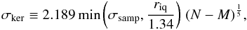 (18)where
σsamp,riq,N
and M are the sample standard deviation, the interquartile range of
the samples, number of samples and burn-in length, respectively.
(18)where
σsamp,riq,N
and M are the sample standard deviation, the interquartile range of
the samples, number of samples and burn-in length, respectively.
Periodogram mode.
By default, the window width for marginal posteriors is based on the MCMC sample standard deviation σsamp (Eq. (18)). If there are multiple maxima, however, this can lead to artificially broad peaks, which can be particularly problematic for the orbital frequency f (see Sect. 2.3), which plays an important role in distinguishing different solutions in orbit-related parameter estimation. Therefore, BASE includes a periodogram mode, in which the window width of the marginal posterior of f (a Bayesian analogon to the frequentist periodogram) is reduced according the following procedure.
-
1.
Initially assume a default window width as given byEq. (18);
-
2.
estimate the marginal posterior of f and find its local maximum fmax nearest to posterior mode
 ,
as well as the local minimum fmin nearest to
fmax;
,
as well as the local minimum fmin nearest to
fmax; -
3.
calculate the marginal-posterior standard deviation σ′ over the half-peak between fmax and fmin;
-
4.
re-calculate the window width using Eq. (18), with
 replacing
σsamp;
replacing
σsamp; -
5.
repeat step 2, but only consider local minima with ordinates
 in order not to be misled by weak marginal-posterior fluctuations;
 -
6.
repeat steps 3 and 4.
Model parameters used by BASE.
Quantities derived from model parameters.
Parameter estimation.
To obtain a single most probable estimate of the parameters, the posterior
density
can be summarised by the posterior mode  , i.e. the point where the posterior
assumes its maximum value,
, i.e. the point where the posterior
assumes its maximum value, 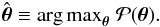 (19)This point, also known as the maximum
a-posteriori (MAP) parameter estimate, can be approximated by the MCMC sample with
highest posterior density, based on the values of
(19)This point, also known as the maximum
a-posteriori (MAP) parameter estimate, can be approximated by the MCMC sample with
highest posterior density, based on the values of
 already calculated during sampling. This approximation neglects the finite spacing
between samples.
already calculated during sampling. This approximation neglects the finite spacing
between samples.
Alternatively, the following scalar summaries can be inferred from the samples or,
for the marginal mode, from the marginal
posteriors  :
:
-
mean or expectation
 ,
,
 (20)
(20) -
median
 ,
,
 (21)
(21) -
marginal mode
 ,
,
 (22)
(22)
Uncertainty estimation.
For uncertainty estimation, highest posterior-density intervals (HPDIs) can be
derived from the posterior samples. For any given C ∈ R with
0 < C < 1, a
HPDI IHPD ≡ [a,b] is defined as the
smallest interval over which the posterior contains a probability C,
 (23)BASE automatically calculates HPDIs of
probability contents 50%, 68.27%, 95%, 95.45%, 99%, and 99.73%; others may be added on
user request.
(23)BASE automatically calculates HPDIs of
probability contents 50%, 68.27%, 95%, 95.45%, 99%, and 99.73%; others may be added on
user request.
In contrast to frequentist confidence intervals, HPDIs are generally not symmetric, meaning that their midpoint does not correspond to the best estimate. This is because the marginal posteriors may be asymmetric, including any amount of skew.
It should also be noted that HPDIs are not useful with multimodal posteriors because several modes cannot be meaningfully summarised by one interval per dimension, nor by a single best estimate.
To quantify linear dependencies between parameters, the a posteriori Pearson
correlation coefficient, 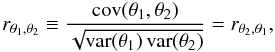 (24)can be inferred from the samples. There
may also be nonlinear correlations between parameters that are not described by the
correlation coefficients. One should also be aware that for strong linear or
non-linear relationships between parameters, uncertainties of single parameters as
characterised by HPDIs may not be meaningful.
(24)can be inferred from the samples. There
may also be nonlinear correlations between parameters that are not described by the
correlation coefficients. One should also be aware that for strong linear or
non-linear relationships between parameters, uncertainties of single parameters as
characterised by HPDIs may not be meaningful.
We stress that the (joint) marginal posteriors can – and should – always be referred to, especially when best estimates and/or HPDIs do not adequately characterise the posterior. The availability of these more informative densities is one of the advantages of a Bayesian approach with posterior sampling.
2.3. Observable models
Independent of the chosen approach to inference – frequentist or Bayesian –, theoretical values of the observables need to be calculated and compared to the data by means of the likelihood. To this end, an observable model is set up for each relevant type of data, i.e. a function f(θ;t) of the model parameters θ and time t. An overview of all model parameters used in this work is given in Table 1, while Table 2 lists quantities that can be derived from them.
In this section, we only sketch the derivation of the observable models, beginning with a single-planet system. For an in-depth treatment of celestial mechanics, the interested reader is referred e.g. to Moulton (1984).
2.3.1. Stellar motion in the orbital plane
Newton’s Law of Gravity governs the motion of a non-relativistic two-body system of star and planet, whose centre of mass (CM) rests in some inertial reference frame. A solution to it is given by both the star and the planet moving in elliptical Keplerian orbits with a fixed common orbital plane and each with one focus coinciding with the CM.
To describe the stellar position, whose variation is observable with astrometry and
Doppler spectroscopy, we set up a coordinate system S1 whose
origin is identical to the CM, z-axis perpendicular to the orbital
plane and the vector from the CM to the periapsis orientated in positive
x-direction. In S1, the stellar
barycentric position is given by 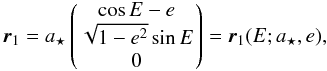 (25)where
a⋆ is the semi-major axis,
e the eccentricity and E the eccentric anomaly.
(25)where
a⋆ is the semi-major axis,
e the eccentricity and E the eccentric anomaly.
The time-dependent eccentric anomaly is determined implicitly by Kepler’s equation,
 (26)where
f = P-1 is the orbital frequency,
P the orbital period, t1 the time of
first measurement and M(·) the mean anomaly, which varies uniformly
over the course of an orbit. Furthermore, following Gregory (2005a), we use
(26)where
f = P-1 is the orbital frequency,
P the orbital period, t1 the time of
first measurement and M(·) the mean anomaly, which varies uniformly
over the course of an orbit. Furthermore, following Gregory (2005a), we use 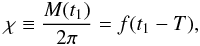 (27)with T standing for the
last time the periapsis was passed prior to t1 (time of
periapsis). Kepler’s equation is transcendental and needs to be solved numerically to
obtain E for every relevant combination of e and
M.
(27)with T standing for the
last time the periapsis was passed prior to t1 (time of
periapsis). Kepler’s equation is transcendental and needs to be solved numerically to
obtain E for every relevant combination of e and
M.
BASE performs a one-time pre-calculation of E over an (e,M)-grid, which, because of the monotonicity of E as an (implicit) function of e and M, allows one to reduce the effort of numerically solving Eq. (26) by providing lower and upper bounds on E.
By reference to Eqs. (25) and (26), it is readily shown that the stellar coordinates are periodic functions of χ with period 1. We therefore call χ a cyclic parameter and treat it as lying in the range [0,1).
2.3.2. Transformation into the reference system
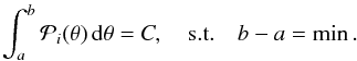
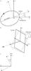 |
Fig. 1 Definition of the angles ω⋆,i,Ω. a) From S1 to S2, the star and its sense of rotation about the CM are indicated; the dotted line marks the major axis of the orbital ellipse. b) From S2 to S3, the observer and line of sight are indicated. c) From S3 to S4, the positive x4-axis points northward along the meridian of the CM. |
To derive the stellar barycentric position as seen from the perspective of an observer, we transform S1 into a new coordinate system S4 by three successive rotations. These are described by three Euler angles, termed in our case argument of the periapsis ω⋆, inclination i and position angle of the ascending node Ω, and are carried out as follows (Fig. 1):
-
1.
Rotate S1 about its z1-axis by (−ω⋆) such that the ascending node 4 of thestellar orbit lies on the positive x2-axis.
-
2.
Rotate S2 about its x2-axis by (+ i) such that the new z3-axis passes through the observer.
-
3.
Rotate S3 about its z3-axis by (− Ω) such that the new x4-axis is parallel to the meridian of the CM and points in a northern direction.
Thus, the stellar barycentric position has new coordinates 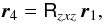 (28)with matrix
 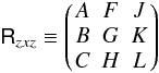 (29)defining the rotations; its components are
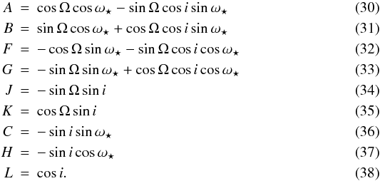 A,B,F,and
G are known as the Thiele-Innes constants, first introduced by Thiele (1883).
A,B,F,and
G are known as the Thiele-Innes constants, first introduced by Thiele (1883).
By taking the time derivative of Eq. (28), we obtain the stellar velocity in S4,
 (39)
(39)
2.3.3. Relation to the planetary orbit
By reference to the above results, the observables of AM and RV are easily derived (Sect. 2.3.4). Based on the following simple relation, they can be parameterised by quantities pertaining to the planetary instead of the stellar orbit.
According to the definition of the CM, the line connecting star and planet contains the
CM and the ratio of their respective distances from the CM equals the inverse mass
ratio,  (40)where C, S and P stand for CM, star and
planet, respectively. This implies a simple relation between the orbits of the star and
the planet as follows. The two bodies orbit the CM with a common orbital
frequency f and time of periapsis T. With regard to
the corresponding periapsis, they always have the same eccentric
anomaly E. Their orbital shapes, viz.
eccentricities e, are identical as well.
(40)where C, S and P stand for CM, star and
planet, respectively. This implies a simple relation between the orbits of the star and
the planet as follows. The two bodies orbit the CM with a common orbital
frequency f and time of periapsis T. With regard to
the corresponding periapsis, they always have the same eccentric
anomaly E. Their orbital shapes, viz.
eccentricities e, are identical as well.
Furthermore, the two bodies share the same sense of orbital revolution, hence those nodes of both orbits which lie on the positive x2-axis are ascending. Consequently, the only Euler angle that differs between stellar and planetary orbit is the argument of periapsis, which differs by π because star and planet are in opposite directions from the CM.
2.3.4. Observables
To express the stellar barycentric position as a two-dimensional angular position, we
performed a final transformation of S4 into a spherical
coordinate system S5 with radial, elevation and azimuthal
coordinates (r,δ,α). Its origin is identical with the observer, its
reference plane coincides with the
(y4,z4)-plane and its fixed
direction is −z4. In S5, the
radial coordinate of the CM equals a
distance d = 1AU ϖ-1, with
ϖ being the parallax. Stellar coordinates
r4 therefore correspond to a two-dimensional
angular position  (41)in S5, where
δ and α are called the declination and right
ascension, respectively. Using Eqs. (25), (28) and (29), the model function for the angular
position of the star with respect to the CM becomes
(41)in S5, where
δ and α are called the declination and right
ascension, respectively. Using Eqs. (25), (28) and (29), the model function for the angular
position of the star with respect to the CM becomes  (42)with
a′ ≡ ϖa⋆(1AU)-1.
In practice, complications arise because the stellar position is often measured relative
to a physically unattached reference star, whose distance and motion differ, and not
relative to the unobservable CM. By contrast, for a visual binary, the companion can be
used as a reference, yielding the simple model described below.
(42)with
a′ ≡ ϖa⋆(1AU)-1.
In practice, complications arise because the stellar position is often measured relative
to a physically unattached reference star, whose distance and motion differ, and not
relative to the unobservable CM. By contrast, for a visual binary, the companion can be
used as a reference, yielding the simple model described below.
Other astrometric effects may be caused by the accelerated motion of Earth-bound observers around the solar system barycentre (SSB). This is discussed for the case of the binary Mizar A in Sect. 2.3.5.
In contrast to astrometry, RV data are usually automatically transformed into an
inertial frame resting with respect to the SSB (e.g. Lindegren & Dravins 2003), which allows the Earth’s motion to be neglected
in this model and treats the observer’s rest frame as being inertial. The model function
for the stellar radial velocity measured by an observer is thus given by
 , with
 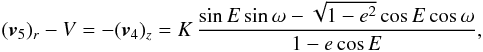 (43)where V is the RV offset,
consisting of the radial velocity of the CM plus an offset due to the specific
calibration of the instrument – which therefore differ, in general, between RV data
sets – and K is the RV semi-amplitude, which can be expressed as
(43)where V is the RV offset,
consisting of the radial velocity of the CM plus an offset due to the specific
calibration of the instrument – which therefore differ, in general, between RV data
sets – and K is the RV semi-amplitude, which can be expressed as
![Mathematical equation: \begin{equation} K = 2\pi\PMf\PMaS\sin\PMi = \sqrt[3]{2\pi\gravConst\PMf}\,\PMmP(\PMmP+\PMmS)^{-\frac{2}{3}}\sin\PMi.\label{eq_RV_amplitude_II} \end{equation}](/articles/aa/full_html/2012/09/aa19074-12/aa19074-12-eq227.png) (44)The last equality holds because of Kepler’s
third law,
(44)The last equality holds because of Kepler’s
third law, 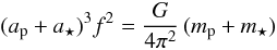 (45)and the definition of the CM (Eq. (40)). Owing to Eq. (44), only one of
a⋆,K needs to be
employed in the AM and RV models; for BASE, K was adopted.
(45)and the definition of the CM (Eq. (40)). Owing to Eq. (44), only one of
a⋆,K needs to be
employed in the AM and RV models; for BASE, K was adopted.
As an aside, in the literature (e.g. Gregory
2005a) often a different version of Eq. (43) is employed that involves ν instead of
E and the alternative definition
 (see Table 2).
Binary system.
If the primary and secondary binary components assume the roles of star and planet, respectively, the above reasoning also yields the observables of a binary system.
For visual binaries, AM measurements often refer to the position of the secondary
with respect to the primary. From the definition of the CM, it follows that the orbit
of the secondary with respect to the primary is identical with its barycentric orbit
but scaled by a factor  , or with the semi-major axis equaling
the sum of the two components’ barycentric semi-major axes,
, or with the semi-major axis equaling
the sum of the two components’ barycentric semi-major axes, 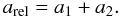 (46)Thus, the AM model of Eq. (42) can be used for a binary
with arel replacing
a⋆,
ω2 + π replacing
ω⋆ and
(46)Thus, the AM model of Eq. (42) can be used for a binary
with arel replacing
a⋆,
ω2 + π replacing
ω⋆ and 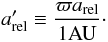 (47)Equation (43) yields the RV of component i if
K is replaced by
(− 1)i + 1Ki
and ω by ω2. If AM and RV data are
combined, BASE uses K1,2 instead of
a1,2 and calculates arel
using the equivalent of Eq. (44) in
combination with Eq. (46).
(47)Equation (43) yields the RV of component i if
K is replaced by
(− 1)i + 1Ki
and ω by ω2. If AM and RV data are
combined, BASE uses K1,2 instead of
a1,2 and calculates arel
using the equivalent of Eq. (44) in
combination with Eq. (46).
2.3.5. Effects of the motion of observer and CM
If we consider the observer, whose position relative to the CM defines the orientation of S2......11...5, to be located on Earth and therefore to be subject to Earth’s accelerated motion around the SSB, the angles Ω,i,ω as defined above are not constant but rather functions of time; an additional source of their variation is the (assumedly linear) proper motion of the CM. Consequently, these angles are not appropriate constant model parameters even within a timespan of a few months. Furthermore, the systems S2......11...5 defined above are not strictly inertial, which renders the simple coordinate transformations invalid. However, we argue below that the variation in these angles is so weak that these effects are indeed negligible in the context of this work.
Because AM determines instantaneous positions, it is directly influenced by changes in the positions of the observer and the CM. In the following, we assess for Mizar A the greatest possible magnitude of a change in the AM position Δr ≡ |Δr| due to angular changes ΔΩ,Δi,Δω > 0, which are in turn caused by the varying relative position of observer and CM. Finally, we compare Δr to the AM measurement uncertainties.
An upper limit on each of the angular changes
ΔΩ,Δi,Δω can be derived from the proper motion of
the CM and the annual parallax from the Earth’s motion, as  (48)where the first term corresponds to the
annual parallax and μ is the magnitude of the CM’s proper motion. For
the second term, we have
(48)where the first term corresponds to the
annual parallax and μ is the magnitude of the CM’s proper motion. For
the second term, we have  .
.
Using
sin(x + ξ) ≈ sinx + ξcosx,
for ξ ≪ 1, along with Eqs. (30)–(35) and (48) as well as the final results for
Ω,i,ω and ϖ (using the
values  from Table B.1) and the proper motion from
Table 3 yields the following maximum changes of
the Thiele-Innes constants:
from Table B.1) and the proper motion from
Table 3 yields the following maximum changes of
the Thiele-Innes constants:  Hence, with
 ,
,  and the final posterior
median
and the final posterior
median  (Table B.2), we obtain the maximum change in relative angular position of the two
components,
(Table B.2), we obtain the maximum change in relative angular position of the two
components,  (55)Comparison with Table 4 reveals that this is more than two orders of
magnitude smaller than the median AM measurement uncertainty, proving that the motions
of the Earth and the CM of Mizar A can indeed be neglected.
(55)Comparison with Table 4 reveals that this is more than two orders of
magnitude smaller than the median AM measurement uncertainty, proving that the motions
of the Earth and the CM of Mizar A can indeed be neglected.
Basic physical properties of Mizar A.
Published data for Mizar A used in this work.
3. BASE – Bayesian astrometric and spectroscopic exoplanet detection and characterisation tool
We have developed BASE, a computer program for the combined Bayesian analysis of AM and RV data according to Sect. 2, for the following main reasons.
-
A statistically well-founded, reliable tool was needed that was able to perform a complete Bayesian parameter and uncertainty estimation, along with model selection (only for planetary systems, not detailed in this article).
-
We aimed to combine astrometry and Doppler-spectroscopy analyses.
-
A possibility to include knowledge from earlier analyses was needed.
-
Finding all relevant solutions across a multidimensional, high-volume parameter space Θ was required. A more detailed knowledge of the parameters than a best estimate and a confidence interval can provide is especially important when the data do not constrain the parameters well, e.g. when only few data have been recorded or the signal-to-noise ratio is low (as can be the case for lightweight planets or young host stars).
BASE is a highly configurable command-line tool developed in Fortran 2008 and compiled with GFortran (Free Software Foundation 2011a). Options can be used to control the program’s behaviour and supply information such as the stellar mass or prior knowledge (see Sect. 3.1). Any option can be supplied in a configuration file and/or on the command line.
3.1. Prior knowledge
Any model parameter can be assigned a prior probability density in one of three forms:
-
a fixed value;
-
a user-defined shape, i.e. a set
 ;
;
-
a range (either in combination with a specific shape, which is then clipped to the given range, or else using one of the standard prior shapes detailed in Sect. A).
Any parameter for which no such option is present is assigned a default prior shape and range to pose the weakest possible restraints justified by the data, the model, and mathematical/ physical considerations.
3.2. Physical systems and modes of operation
As mentioned above, BASE is capable of analysing data for two similar types of systems, whose physics have been described in Sect. 2.3. These are systems with
-
1.
one observable component that may be accompanied by one ormore unobserved bodies (generally referred to as planetarysystems here for simplicity); in this normal mode, the number ofcompanions can be set to a value ranging from zero to nine, or a listof such values, in which case several runs are conducted and theoutcome is compared in terms of model selection;
-
2.
two observable, gravitationally bound components (referred to as binary stars); this mode of operation is called binary mode.
3.3. Types of data
Observational data of the following types can be treated by BASE:
-
AM data, whose observable, in the case of binary targets, is therelative angular position of the two binary components. Each datarecord consists of a date, the angular position(αcosδ,δ) or (ρ,θ) in a cartesian or polar coordinate system, and its standard uncertainty ellipse, given by (a,b,φ);
-
RV data, where each data record consists of a date and the observed stellar radial velocity as well as its uncertainty.
3.4. Computational techniques
In the following, we describe some computational techniques implemented in BASE that are relevant to the present work.
Improved exploration of parameter space.
To enhance the mixing, i.e. rapidness of exploration of the parameter space, of Markov
chains produced by the Metropolis-Hastings (MH) algorithm (Sect. 2.2.2) and decrease their attraction by local posterior modes, the
parallel tempering (PT) algorithm (e.g. Gregory
2005b) is employed one level above MH. Its function is to create in parallel
n chains of length N,
 each sampled by an independent MH
procedure, where the cold chain k = 1 uses an unmodified
likelihood ℒ(·), while the others, the heated chains, use as replacement
ℒ(·)γ(k) with the positive
tempering parameter γ(k) < 1. After
nswap samples of each chain, two chains
k ≥ 1 and k + 1 ≤ n are randomly
selected and their last links, denoted here by
θ(k) and
θ(k + 1), are swapped with
probability
each sampled by an independent MH
procedure, where the cold chain k = 1 uses an unmodified
likelihood ℒ(·), while the others, the heated chains, use as replacement
ℒ(·)γ(k) with the positive
tempering parameter γ(k) < 1. After
nswap samples of each chain, two chains
k ≥ 1 and k + 1 ≤ n are randomly
selected and their last links, denoted here by
θ(k) and
θ(k + 1), are swapped with
probability  (56)which ensures that the distributions of
both chains remain unchanged.
(56)which ensures that the distributions of
both chains remain unchanged.
This procedure allows states from the “hotter” chains, which explore parameter space more freely, to “seep through” to the cold chain without compromising its distribution. Conclusions are only drawn from the samples of the cold chain.
In contrast to MCMC sampling, which is sequential in nature, the structure of PT allows one to exploit the multiprocessing facilities provided by many modern computing architectures. For this purpose, BASE uses the OpenMP API (OpenMP Architecture Review Board 2008) as implemented for GFortran by the GOMP project (Free Software Foundation 2011b).
Assessing convergence.
As a matter of principle, it cannot be proven that a given Markov chain has converged to the posterior. However, convergence may be meaningfully defined as the degree to which the chain does not depend on its initial state θ(0) any more. This can be determined on the basis of a set of independent chains – in our case, the cold chains of m independent PT procedures – started at different points in parameter space. These starting states should be defined such that for each of their components, they are overdispersed with respect to the corresponding marginal posteriors.
Since the marginal posteriors are difficult to obtain before the actual sampling, BASE determines the starting states by repeatedly drawing, for each parameter, a set of m samples from the prior using rejection sampling; the repetition is stopped as soon as the sample variance exceeds the corresponding prior variance, which yields a set of starting states overdispersed with respect to the prior. Assuming that the prior variance exceeds the marginal-posterior variance, the overdispersion requirement is met.
Such a test, using the potential scale reduction (PSR) or Gelman-Rubin statistic, was proposed by Gelman & Rubin (1992) and was later refined and corrected by Brooks & Gelman (1998). It is repeatedly carried out during sampling and, in the case of a positive result, sampling is stopped before the user-defined maximum runtime and/or number of samples have been reached. It may also sometimes be useful to abort sampling manually, which can be done at any time.
The statistic is calculated with respect to each parameter θ
separately, using the post-burn-in samples5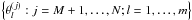 of θ provided by the
m independent chains. It compares the actual variances of
θ within the chains built up thus far to an estimate of the
marginal-posterior (i.e. target) variance of θ, thus estimating how
closely the chains have approached convergence.
of θ provided by the
m independent chains. It compares the actual variances of
θ within the chains built up thus far to an estimate of the
marginal-posterior (i.e. target) variance of θ, thus estimating how
closely the chains have approached convergence.
The PSR is defined as 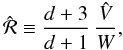 (57)where
 is an estimate of the marginal-posterior variance, d the estimated
number of degrees of freedom underlying the calculation of
,
and W the mean within-sequence variance. The quantities are defined as
is an estimate of the marginal-posterior variance, d the estimated
number of degrees of freedom underlying the calculation of
,
and W the mean within-sequence variance. The quantities are defined as
 \arraycolsep1.75ptwhere B
is the between-sequence variance and
ν ≡ N − M; a horizontal bar denotes
the mean taken over the set of samples obtained by varying the omitted indexes.
\arraycolsep1.75ptwhere B
is the between-sequence variance and
ν ≡ N − M; a horizontal bar denotes
the mean taken over the set of samples obtained by varying the omitted indexes.
Owing to the initial overdispersion of starting states,
overestimates the marginal-posterior variance in the beginning and subsequently
decreases. Furthermore, while the chains are still exploring new areas of parameter
space, W underestimates the marginal-posterior variance and increases.
Thus, as convergence to the posterior is accomplished, . Therefore, we can assume
convergence as soon as the PSR has fallen below a threshold . If BASE is run with
ℛ ∗ ≡ 1, sampling is continued up to the user-defined length or duration,
respectively.
For cyclic parameters (Sect. 2.3), the default lower and upper prior bounds are equivalent, which needs to be taken into account when calculating the PSR. Thus, BASE uses the modified definition of the PSR by Ford (2006) for these parameters.
4. Target and data
Mizar A (ζ1 Ursae
Majoris, HD 116656, HR 5054), the first spectroscopic binary discovered, is of
double-lined type (SB II; Pickering 1890). Its basic
physical properties are summarised in Table 3.
Together with the spectroscopic binary Mizar B, it
forms the Mizar quadruple system, seen from Earth
as a visual binary with the components separated by about
 . Mizar is the first double star discovered
by a telescope and also the first one to be imaged photographically (Bond 1857).
. Mizar is the first double star discovered
by a telescope and also the first one to be imaged photographically (Bond 1857).
At an apparent angular separation of about  , or 74 ± 39 kAU spatial distance, Mizar is
accompanied by Alcor, which has recently turned out to be a spectroscopic binary itself
(Mamajek et al. 2010). Mizar and Alcor, also known
as the “Horse and Rider”, form an easy naked-eye double star, while it is still a matter of
debate whether or not they constitute a physically bound sextuplet.
, or 74 ± 39 kAU spatial distance, Mizar is
accompanied by Alcor, which has recently turned out to be a spectroscopic binary itself
(Mamajek et al. 2010). Mizar and Alcor, also known
as the “Horse and Rider”, form an easy naked-eye double star, while it is still a matter of
debate whether or not they constitute a physically bound sextuplet.
Published data used in this article are displayed in Figs. 7, 8 along with the model functions determined by BASE and their properties are summarised in Table 4. Using a Coudé spectrograph at the 1.93-m telescope at Observatoire Haute Provence, Prevot (1961) obtained 17 optical photographic spectra of the light of Mizar A combined with that of electric arcs or sparks between iron electrodes. For each of the 13 individual stellar lines identified in the spectra, one intermediate radial-velocity value per binary component was obtained by comparison with a set of reference lines of iron. Finally, a set of 17 pairs of RVs for the two components was calculated as arithmetic means of the corresponding intermediate values. The RV measurement uncertainty is not given by Prevot (1961) and was therefore estimated in the course of the present work, as described in Sect. 5.
High-precision AM data of Mizar A were first obtained by Hummel et al. (1995) using the Mark III optical interferometer on Mount Wilson, California (Shao et al. 1988), with baseline lengths between 3 and 31 m. It measured the squared visibilities and their uncertainties at positions sampled over the aperture plane due to Earth’s rotation. The visibilities can be modelled as a function of the diameters, magnitude differences, and relative angular positions (ρ,θ) of the binary components, Armstrong et al. (1992). These authors also describe a procedure to derive one angular position for each night of observation from a corresponding set of visibilities, which was adopted by Hummel et al. (1995) to obtain initial estimates of the orbital parameters. These positional data are also relevant for the present work. Hummel et al. (1995) also performed a direct fit to the squared visibilities to derive final estimates of the component diameters and orbital parameters.
Later, a descendant instrument, the Navy Prototype Optical Interferometer (NPOI) at Lowell observatory, Arizona (Armstrong et al. 1998), was used by Hummel et al. (1998) to obtain more accurate results using three siderostats, viz. three baselines at a time. This allowed a better calibration using the closure phase6, which is independent of atmospheric turbulence. Similarly as before, Hummel et al. (1998) separately fitted binary orbits directly to the visibility data and also to the positional angles derived for each night, concluding that the respective results agree well with each other and that those parameters in common with spectroscopic analyses are compatible with Prevot (1961); they also performed a fit to both AM and RV data to obtain their final parameter estimates.
While Hummel et al. (1998) did not include the older, less accurate Mark III data in their analysis, we present a combined treatment of all published data, i.e. the AM positions of Hummel et al. (1995) and Hummel et al. (1998) along with the RV data of Prevot (1961).
5. Analysis and results
Analysis passes carried out sequentially.
To illustrate the features of BASE and demonstrate its validity, we used the tool to analyse all published data of Mizar A. This section details the steps taken in and the results of our analysis. Its general goal was, given uninformative prior knowledge, to search the parameter space as comprehensively as possible to find and characterise the a posteriori most probable solution together with its uncertainty and other characteristics. For reasons detailed below, once the RV data had been prepared, several runs of BASE (Table 5) were manually conducted, each using priors derived from the previous pass, with relatively uninformative priors in the first step.
In this analysis, our approach was to regard all nominal measurement uncertainties as accurate by setting parameters characterising additional noise in AM (τ+) as well as RV (σ+) data to zero.
Astrometric data alone allow one to constrain neither the RV offset V nor the amplitudes K1,K2 but only the sum K1 + K2 (Sect. 2.3.4). By contrast, these parameters can be constrained using spectroscopic data alone, or AM and RV data both. However, the AM data reduce the relative weight of the spectroscopic data and thus make the determination of these parameters harder. We found in the course of this work that by an iterative approach, starting with a first pass using only RV data, this difficulty could be resolved.
In all passes, BASE was configured to build up eight parallel chains, including the cold chain, using the parallel-tempering technique (detailed in Sect. 3.4). 108 posterior samples were collected, the first 10% of which were assumed to be burn-in samples. In the final pass, two PT procedures were employed to enable a test of convergence to the posterior, which reduced the number of samples collected with unchanged memory requirements to 5 × 10⁷. Convergence was not assessed in earlier passes, because convergence was difficult to reach as long as several distinct solutions existed within the prior support.
5.1. Preparation of RV data
Assuming appropriate measurement uncertainties is a prerequisite for the proper relative weighting of the different data types when combining them. Because these uncertainties are not quoted by Prevot (1961) for the spectroscopic data, we estimated them according to the following method.
First, we assumed that each RV datum vi is
the sum of the model
value v(θtrue;ti)
and an error ei, where
θtrue are the true parameter values and the
errors are independent and identically Gaussian-distributed with an unknown standard
deviation σ. Furthermore, we assumed that the model parameters found in
a particular analysis are identical with θtrue.
It follows that the uncertainty σ can be estimated as the sample standard
deviation of the set of residuals  .
.
Thus, based on the sample standard deviation of the best-fit residuals of Prevot (1961), viz. 2.13 km s-1, we
initially assumed a conservative value of 2.50 km s-1 for all data. To
quantify the measurement uncertainties based on our own inference, we then conducted a
preliminary analysis similar to pass A described in the next subsection, from which we
finally inferred σ = 2.05 km s-1. In addition, we took a
more correct alternative approach to estimating the RV uncertainties by assuming a
relatively low value of σ = 2.00 km s-1 and allowing for
higher noise via σ+, which led to an estimate
 deviating by less than 1.7% from our
previous estimate.
deviating by less than 1.7% from our
previous estimate.
5.2. Pass A: first constraints on RV parameters
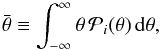
Pass A: initial prior ranges.
 |
Fig. 2 Pass A: marginal posteriors of RV amplitudes K1 (top, solid line), K2 (top, dashed line) and offset V (bottom), all plotted over the approximate range of the corresponding 99% HPDI. |
To facilitate the determination of the RV parameters K1,K2 and V, a first pass using only RV data was carried out, as mentioned above. It used uninformative priors (Sect. A and Table 1), with bounds listed in Table 6.
Figure 2 shows the resulting marginal posteriors (see Sect. 2.2.2) of the RV offset V and the amplitudes K1,K2, with the abscissae approximately corresponding to the 99% HPDIs. These marginal posteriors represent much tighter constraints on the parameters than the corresponding priors do.
5.3. Pass B: combining all data
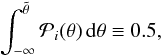
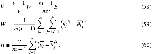
Providing as new priors the marginal posteriors of all RV parameters e,f,χ,ω2,V,K1 and K2 from pass A, constrained to the corresponding 99% HPDIs IHPD,99%, and again using uninformative priors on the additional parameters (Table 7), the AM data were added and BASE was run again. Using the resulting posterior samples, BASE was additionally invoked in periodogram mode to refine the kernel window width for the marginal posterior of f as described in Sect. 2.2.2. (This refinement was not used in pass A in order not to constrain the frequency too tightly before adding the AM data, because the combined data are expected to correspond to a marginally differing frequency.)
The resulting marginal posterior (Fig. 3) exhibits a very strong mode around 0.04869 d-1, whose height is 8.1 times that of the next lower peak. Over the range of its mode, the marginal posterior contains a total probability of 45.0%. Most other parameters in this stage have very broad and/or multimodal marginal posteriors, hinting at different solutions still probable within the prior support.
Pass B: prior ranges for additional AM parameters.
 |
Fig. 3 Pass B: marginal posterior of orbital frequency f, plotted over the range of the corresponding 99% HPDI. This is a Bayesian analogon to the frequentist periodogram. |
5.4. Pass C: selecting the frequency f
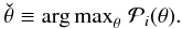
For the next pass, the prior of f was provided by the marginal posterior of pass B (Fig. 3), constrained to the range of the marginal mode. For all other parameters, priors were identical with the previous marginal posteriors, constrained to IHPD,99%.
With the frequency thus restrained, the pass produced unimodal marginal posteriors in all parameters except for ω2 and Ω.
The marginal posteriors of the argument of periapsis ω2 and the position angle of the ascending node Ω exhibited small local maxima located at a distance of −1.02π and + 1.03π from their marginal modes, respectively (indicated by triangles in Fig. 4). This can be explained by the fact that the Thiele-Innes constants (Eqs. (30)–(33)), which appear in the AM model, contain products of sin(·) and/or cos(·) functions with ω2 and Ω as arguments. These products retain their values when ω2 and Ω are both shifted by π – with opposite signs, since the marginal modes of these angles lie in different halves of the interval [0,2π). Consequently, the AM model function is invariant with respect to such shifts. (Thus, when analysing only AM data, it cannot be determined which node is ascending, hence Ω is defined only over the interval [0,π) and refers to the first node.) Owing to the combination with RV data, which independently constrain ω2 (Eq. (43)), the ambiguity is strongly reduced, as illustrated by the very small subpeaks in Fig. 4 – though it is not completely resolved.
As another result from this pass, the high correlation coefficient of the two angles, rω2,Ω = −0.62, expresses the strong negative linear relationship between them introduced by the possibility of a contrarious change.
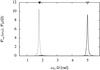 |
Fig. 4 Pass C: marginal posteriors of the argument of periapsis ω2 (solid line) and position angle of the ascending node Ω (dashed line), plotted over the approximate range of the corresponding 99% HPDIs. Triangles indicate the positions of small local maxima located approximately ± π from the corresponding marginal modes. |
5.5. Passes D and E: selecting ω2 and Ω and refining results
In pass D, the ambiguity in ω2 and Ω was resolved by selecting the range around their marginal modes via the new priors. For all other parameters, priors were again identical to the previous marginal posteriors, constrained to IHPD,99%. All resulting marginal posteriors turned out to be unimodal, corresponding to a single solution as opposed to several clearly distinct orbital solutions.
As a final step, pass E was conducted to refine the results by using all previous marginal posteriors, constrained to IHPD,99%, as new priors, thus confining the parameter space a priori to the most probable solution.
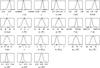 |
Fig. 5 Marginal posteriors of parameters e,f,χ,ω2,i,Ω,ϖ,V,K1,K2 (see also Table 1) and derived quantities P,T,d,ρ,Kalt,1,Kalt,2,m1,m2,a1,a2,arel (Table 2) with marginal-posterior medians (dotted line) and 68.27% HPDIs (dashed lines), from the final pass. Abscissae ranges are identical with the corresponding 95% HPDIs. Ordinate values were omitted but follow from normalisation. Open triangles on the upper abscissae indicate the MAP estimates. Open circles on the lower abscissae bound the confidence intervals given by or derived from Prevot (1961), while open triangles refer to the intervals of Hummel et al. (1998). Some of these literature estimates are not plotted because they are outside the abscissa range; for f and χ, no literature uncertainty estimate is available. For derivations and numerical values, see Tables B.1 and B.2. |
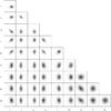 |
Fig. 6 Two-parameter joint marginal posterior
densities |
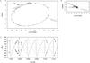 |
Fig. 7 AM and RV data and models calculated with the MAP parameter estimates (Table B.1). a) AM data (uncertainty ellipses, solid lines), model (large ellipse, solid line) and residual vectors (dashed lines). b) Residual AM error ellipses. c) RV data and model for primary (normal error bars, solid line) and secondary (hourglass-shaped error bars, dotted line). The horizontal dashed line indicates the RV offset V. RV residuals are presented in Fig. 8. |
 |
Fig. 8 All data types: from top to bottom: AM data and model (δ coordinate); AM residuals Δδ; AM data and model (αcosδ coordinate); AM residuals Δ(αcosδ); RV data and model v (primary: solid line, secondary: dotted line, RV offset V: horizontal dashed line); RV residuals Δv (primary: normal error bars, secondary: dashed error bars, model: dashed line). AM error bars are defined as the sides of the smallest rectangle orientated along the coordinate axes and containing the respective error ellipse. Abscissa values are mean anomalies M (Eq. (26)), i.e. times folded with respect to the MAP estimates of the time of periapsis T and period P. |
 |
Fig. 9 Distribution of normalised residuals of AM data (long-dashed line), RV data
(short-dashed) and all data (solid), along with the standard normal
distribution |
(Joint) marginal posteriors and correlations.
The final marginal posteriors of all model parameters, plotted over the corresponding 95% HPDIs, are shown in Fig. 5, along with the medians, 68.27% HPDIs (corresponding in probability content to the frequentist 1-σ confidence intervals) and MAP estimates. For comparison, literature estimates and confidence intervals are also included, where permitted by the abscissa range.
Linear and nonlinear dependencies between a pair of parameters may be qualitatively judged by means of the joint marginal posteriors (Sect. 2.2.2) shown in Fig. 6. The inclinations of their equiprobability contours with respect to the coordinate axes are related to the corresponding correlation coefficients. Some joint marginal posteriors exhibit clear deviations from bivariate normal distributions, illustrating that a Gaussian approximation of the likelihood by use of the Fischer matrix (Sect. 2.1) would be inappropriate.
Table B.3 lists the final posterior correlation coefficients. When these attain high absolute values, model-related equations can sometimes serve as an explanation.
For example, the highly negative correlation between f and χ is related to Eq. (26) in the following way. Given data and estimated model parameters, let tm be the time midway between the first and last observations, and Em the eccentric anomaly at tm. Now increase f by a small amount. This can be balanced by a small decrease of χ (or, equivalently, by increasing the time of periapsis T) such that the eccentric anomaly at tm again equals Em. This contrarious change of f and χ, as opposed to leaving only one of them altered, will make E deviate less, on average, over the total timespan; i.e. the model will fit the data better. The relation between f and χ so introduced is indicated by their negative correlation coefficient.
As another example, the highly negative correlation coefficient
ω2 and Ω can be understood by reference to Eqs. (30)–(33), which describes the Thiele-Innes constants of the AM model as
follows. In the case of edge-on orbits (inclination i = 0), these
expressions simplify to sums or differences of cos(·) and sin(·) functions, the
arguments being ω2 + Ω or
ω2 − Ω, with both arguments appearing equally often. An
additional simplification is observed for face-on orbits
( ), where the Thiele-Innes constants are
A = G = −cos(Ω + ω2) and
B = −F = −sin(Ω + ω2).
Thus, for orbits nearly face-on, the strong appearance of the
sum Ω + ω2 introduces a negative correlation between the
two angles, because their contrarious change can lead to the same value of the model
function. For Doppler-spectroscopic data, this is counteracted by the fact that the RV
model function does not contain Ω.
), where the Thiele-Innes constants are
A = G = −cos(Ω + ω2) and
B = −F = −sin(Ω + ω2).
Thus, for orbits nearly face-on, the strong appearance of the
sum Ω + ω2 introduces a negative correlation between the
two angles, because their contrarious change can lead to the same value of the model
function. For Doppler-spectroscopic data, this is counteracted by the fact that the RV
model function does not contain Ω.
Models and residuals.
Figure 7 presents all data with the models calculated from the MAP estimates listed in Table B.1, as well as residual vectors and error ellipses for astrometry. While this analysis used both the older (Hummel et al. 1995) and newer (Hummel et al. 1998) AM in combination with RV data (Prevot 1961), the AM model is very similar to the one calculated by Hummel et al. (1998, Fig. 11) using only the newer AM data because of the overall agreement in parameters.
Figure 8 shows all data, models and residuals, separately by coordinate for AM. The abscissa corresponds to the mean anomaly M (Eq. (26)), i.e. the plots are folded with respect to a time of periapsis T and period P corresponding to the posterior mode. Again, due to the similarity in parameters, the folded RV plot in Fig. 8 is very similar to the corresponding figure in Prevot (1961).
To assess the distribution of the residuals and compare it to a normal distribution,
thus checking the validity of our noise model, we normalised the residuals of both data
types as follows. For AM, we defined the normalised residual as a signed version of the
Mahalanobis distance (Mahalanobis 1936) between
the observed and the modelled values,  (61)with sign
![Mathematical equation: \begin{equation} s_i \defby \sgn\left((\UNCERTELLphi_i-\RESIDphi_i)(\pi-[\UNCERTELLphi_i-\RESIDphi_i])\right), \end{equation}](/articles/aa/full_html/2012/09/aa19074-12/aa19074-12-eq362.png) (62)where
ϕi and
φi are the position angles of the
residual and of the uncertainty ellipse (see Sect. 2.1), respectively. This definition allows us to write, according to
Eq. (7),
(62)where
ϕi and
φi are the position angles of the
residual and of the uncertainty ellipse (see Sect. 2.1), respectively. This definition allows us to write, according to
Eq. (7),
 (63)For RV data, we define
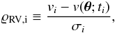 (64)which analogously yields
 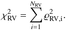 (65)The distributions of normalised residuals
of both data types individually as well as of all data, estimated using kernel density
estimation (Sect. 3.4), are shown in Fig. 9. Table 8 lists
the p-values of the Kolmogorov-Smirnov statistic, which relates each
distribution to the standard normal distribution
(65)The distributions of normalised residuals
of both data types individually as well as of all data, estimated using kernel density
estimation (Sect. 3.4), are shown in Fig. 9. Table 8 lists
the p-values of the Kolmogorov-Smirnov statistic, which relates each
distribution to the standard normal distribution  .
.
The p-value equals the probability, under the
hypothesis  that the normalised residuals are randomly drawn from
,
to observe a distribution of normalised residuals that differs at least as much from
as is actually the case. This difference is quantified here by the Kolmogorov-Smirnov
statistic. Denoting the hypothesis of such an observation by ℋobs, the
p-value can be expressed as
that the normalised residuals are randomly drawn from
,
to observe a distribution of normalised residuals that differs at least as much from
as is actually the case. This difference is quantified here by the Kolmogorov-Smirnov
statistic. Denoting the hypothesis of such an observation by ℋobs, the
p-value can be expressed as  .
We note that according to the Bayes theorem, this is not equal to the “inverse”
probability
.
We note that according to the Bayes theorem, this is not equal to the “inverse”
probability  of the residuals coming from the normal distribution, given the observation.
For the AM residuals, as well as for all residuals, a heavy-tailed distribution
(Fig. 9) is observed and the low
p-value indicates a minute probability of such an observation under
,
i.e. the normalised residuals comply poorly with the standard normal
distribution .
This reflects the fact that several AM data points are outliers with respect to the
observable and noise model (Fig. 7). We interpret
this in terms of systematic effects in the measurements that are not contained in our
noise model. In contrast, the normalised RV residuals are more normally-distributed, and
there are no such severe outliers (Figs. 7 and
8).
According to the principle of maximum entropy, given only the mean and variance of a distribution, the normal distribution has maximum information-theoretic entropy, equivalent to minimum bias or prejudice with respect to the missing information (e.g. Kapur 1989). Still, it is well-known that this widely used noise model is relatively prone to outliers; Lange et al. (1989) have suggested to replace it by a non-standardised t-distribution, resulting in the down-weighting of outliers. This distribution can be derived from the normal distribution under the assumption that the noise variance is unknown with a certain probability distribution. The t-distribution has an additional unknown degrees-of-freedom parameter ν ∈ R; for ν = 1, it resembles the Cauchy-distribution.
In contrast, our approach has been to regard every datum with its standard deviation as accurate, which also implies that we have not discarded any data as outliers. Under this assumption, deviating from the maximum-entropy principle by selecting a different distribution introduces prior “knowledge” that we may not actually have and thus potentially biases the results.
6. Conclusions
We have presented BASE, a novel and highly configurable tool for Bayesian parameter and uncertainty estimation with respect to model parameters and additional derived quantities, which can be applied to AM as well as RV data of both exoplanet systems and binary stars. With user-specified or uninformative prior knowledge, it employs a combination of Markov chain Monte Carlo (MCMC) and several other techniques to explore the whole parameter space and collect samples distributed according to the posterior distribution. We presented a new, simple method of refining the window width of one-dimensional kernel density estimation, which is used to derive marginal posterior densities.
We derived the observable models from Newton’s law of gravitation, neglecting the motion of the observer and the target system, which we showed is justified in the case of Mizar A. After sketching how we estimated the RV uncertainties that are missing in the original publication (Prevot 1961), we detailed our analysis of all publicly available AM and RV data of Mizar A. It consists of five consecutive stages and has produced estimates of the values, uncertainties, and correlations of all model parameters and derived quantities, as well as marginal posterior densities over one and two dimensions.
As illustrated in Fig. 5 and Table B.1, our new results exhibit overall compatibility with previous literature values; this is also the case for the models in Fig. 7, whose plots differ only slightly from those published earlier. Several outliers in the AM data are visible in the distribution of the corresponding normalised residuals, which deviates significantly more from a standard normal distribution than that of the RV residuals. Nevertheless, it is not necessary to remove outliers for our program to finish successfully.
In the near future, we plan to apply BASE to a potential exoplanet host star. In this study one of the aims will be to determine the existence probability of a planetary companion.
Model parameters: new and previous results.
Derived quantities: new and previous results.
Although most methods described in this introduction apply to any kind of companion to a star, we refer here to companions as “exoplanets”, irrespective of whether they are able to sustain hydrogen or deuterium burning.
Throughout, we use the term probability density wherever it refers to a continuous quantity, as opposed to probability for discrete quantities. Probability distribution, denoted by p(·), is a generic term used for both cases.
In general, ti is the value of an independent variable, which may e.g. be temporal or spatial. We assumed the measurement durations to be short in comparison with the characteristic time of orbital motion, given by the orbital period, and thus the observations to take place at points in time ti which are known exactly.
The ascending node is the point of intersection of the orbit and the sky plane where the moving object passes away from the observer. In step 2, a positive rotation angle is used to ensure that the node is indeed ascending (Fig. 1b).
Because the burn-in length M cannot be determined in advance, BASE considers a fixed but configurable fraction of samples to belong to the burn-in phase at any time.
The closure phase φcl is the phase of the product of three visibilities, each pertaining to a different baseline.
Acknowledgments
We wish to thank David W. Hogg, Sabine Reffert, René Andrae, and Mathias Zechmeister for fruitful discussions, and an anonymous referee for comments that have improved the quality and clarity of this article. This research has made use of the SIMBAD database and VizieR catalogue access tool, operated at CDS, Strasbourg, France, as well as NASA’s Astrophysics Data System.
References
- Adamson, A., Aspin, C., Davis, C., et al. 2005, Astronomical Polarimetry: Current Status and Future Directions, ASP Conf. Ser., 343 [Google Scholar]
- Armstrong, J. T., Mozurkewich, D., Vivekanand, M., et al. 1992, AJ, 104, 241 [NASA ADS] [CrossRef] [Google Scholar]
- Armstrong, J. T., Mozurkewich, D., Rickard, L. J., et al. 1998, ApJ, 496, 550 [NASA ADS] [CrossRef] [Google Scholar]
- Bayes, M., & Price, M. 1763, Philosoph. Trans., 53, 370 [Google Scholar]
- Bond, G. 1857, MNRAS, 17, 230 [NASA ADS] [Google Scholar]
- Boneh, A., & Golan, A. 1979, in Third European Congress on Operations Research, EURO III, Amsterdam [Google Scholar]
- Brooks, S. P., & Gelman, A. 1998, J. Computat. Graphic. Statist., 7, 434 [Google Scholar]
- Charbonneau, D., Brown, T. M., Latham, D. W., & Mayor, M. 2000, ApJ, 529, L45 [NASA ADS] [CrossRef] [PubMed] [Google Scholar]
- Deeg, H. J., Belmonte, J. A., & Aparicio, A. 2007, Extrasolar Planets (Cambridge University Press) [Google Scholar]
- Delplancke, F. 2008, New Astron. Rev., 52, 199 [NASA ADS] [CrossRef] [Google Scholar]
- Delplancke, F., Leveque, S. A., Kervella, P., Glindemann, A., & D’Arcio, L. 2000, in SPIE Conf. Ser. 4006, eds. P. Léna, & A. Quirrenbach, 365 [Google Scholar]
- Efron, B., & Tibshirani, R. 1993, An introduction to the bootstrap, Monographs on statistics and applied probability (Chapman & Hall) [Google Scholar]
- Ford, E. B. 2004, in The Search for Other Worlds, eds. S. S. Holt, & D. Deming, ASP Conf. Ser., 713, 27 [Google Scholar]
- Ford, E. B. 2006, ApJ, 642, 505 [NASA ADS] [CrossRef] [Google Scholar]
- Free Software Foundation. 2011a, GFortran, http://gcc.gnu.org/fortran/ [Google Scholar]
- Free Software Foundation. 2011b, GOMP, http://gcc.gnu.org/projects/gomp/ [Google Scholar]
- Gatewood, G., Breakiron, L., Goebel, R., et al. 1980, Icarus, 41, 205 [NASA ADS] [CrossRef] [Google Scholar]
- Gelman, A., & Rubin, D. B. 1992, Stat. Sci., 7, 457 [Google Scholar]
- Geman, S., & Geman, D. 1984, Pattern Analysis and Machine Intelligence, IEEE Transactions on, PAMI-6, 721 [Google Scholar]
- Gilks, W. R., Richardson, S., & Spiegelhalter, D. J. 1996, Markov Chain Monte Carlo in Practice, 1st edn. (London: Chapman & Hall) [Google Scholar]
- Gillessen, S., Eisenhauer, F., Perrin, G., et al. 2010, in SPIE Conf. Ser., 7734 [Google Scholar]
- Gould, A. 2009, in ASP Conf. Ser. 403, ed. K. Z. Stanek, 86 [Google Scholar]
- Gregory, P. C. 2005a, ApJ, 631, 1198 [NASA ADS] [CrossRef] [Google Scholar]
- Gregory, P. C. 2005b, Bayesian Logical Data Analysis for the Physical Sciences: A Comparative Approach with Mathematica Support (Cambridge: Cambridge University Press) [Google Scholar]
- Hastings, W. K. 1970, Biometrika, 57, 97 [Google Scholar]
- Hoffleit, D., & Jaschek, C. 1982, The Bright Star Catalogue (Yale University Observatory) [Google Scholar]
- Holman, M. J., & Murray, N. W. 2005, Science, 307, 1288 [NASA ADS] [CrossRef] [PubMed] [Google Scholar]
- Hummel, C. A., Armstrong, J. T., Buscher, D. F., et al. 1995, AJ, 110, 376 [NASA ADS] [CrossRef] [Google Scholar]
- Hummel, C. A., Mozurkewich, D., Armstrong, J. T., et al. 1998, AJ, 116, 2536 [NASA ADS] [CrossRef] [Google Scholar]
- Kapur, J. 1989, Maximum-Entropy Models in Science and Engineering (Wiley) [Google Scholar]
- Koch, D. G., Borucki, W. J., Basri, G., et al. 2010, ApJ, 713, L79 [NASA ADS] [CrossRef] [Google Scholar]
- Kuhn, J. R., Potter, D., & Parise, B. 2001, ApJ, 553, L189 [NASA ADS] [CrossRef] [Google Scholar]
- Lange, K. L., Little, R. J. A., & Taylor, J. M. G. 1989, J. Am. Statist. Assoc., 84, 881 [Google Scholar]
- Launhardt, R., Queloz, D., Henning, T., et al. 2008, in SPIE Conf. Ser., 7013 [Google Scholar]
- Levine, M., Soummer, R., Arenberg, J., et al. 2009, in The Astronomy and Astrophysics Decadal Survey, 2010, 37 [Google Scholar]
- Lindegren, L., & Dravins, D. 2003, A&A, 401, 1185 [NASA ADS] [CrossRef] [EDP Sciences] [Google Scholar]
- Lovis, C., & Fischer, D. 2010, Radial Velocity Techniques for Exoplanets (University of Arizona Press), 27 [Google Scholar]
- Lyot, B. 1932, ZAp, 5, 73 [Google Scholar]
- Mahalanobis, P. C. 1936, in Proc. National Institute of Science, India, 2, 49 [Google Scholar]
- Mamajek, E. E., Kenworthy, M. A., Hinz, P. M., & Meyer, M. R. 2010, AJ, 139, 919 [NASA ADS] [CrossRef] [Google Scholar]
- Mao, S., & Paczynski, B. 1991, ApJ, 374, L37 [NASA ADS] [CrossRef] [Google Scholar]
- Marois, C., Lafrenière, D., Doyon, R., Macintosh, B., & Nadeau, D. 2006, ApJ, 641, 556 [Google Scholar]
- Mayor, M., & Queloz, D. 1995, Nature, 378, 355 [NASA ADS] [CrossRef] [Google Scholar]
- McArthur, B. E., Benedict, G. F., Barnes, R., et al. 2010, ApJ, 715, 1203 [NASA ADS] [CrossRef] [Google Scholar]
- Metropolis, N., Rosenbluth, A. W., Rosenbluth, M. N., Teller, A. H., & Teller, E. 1953, J. Chem. Phys., 21, 1087 [NASA ADS] [CrossRef] [Google Scholar]
- Moulton, F. 1984, An Introduction to Celestial Mechanics, Dover Books on Astronomy (Dover Publications) [Google Scholar]
- Nascimbeni, V., Piotto, G., Bedin, L. R., & Damasso, M. 2011, A&A, 527, A85 [NASA ADS] [CrossRef] [EDP Sciences] [Google Scholar]
- OpenMP Architecture Review Board. 2008, OpenMP, http://openmp.org/ [Google Scholar]
- Perryman, M. A. C. 2000, Rep. Progr. Phys., 63, 1209 [NASA ADS] [CrossRef] [Google Scholar]
- Perryman, M. A. C., Lindegren, L., Kovalevsky, J., et al. 1997, A&A, 323, L49 [NASA ADS] [Google Scholar]
- Pickering, E. C. 1890, The Observatory, 13, 80 [NASA ADS] [Google Scholar]
- Prevot, L. 1961, J. Observateurs, 44, 83 [NASA ADS] [Google Scholar]
- Reffert, S. 2009, New Astron. Rev., 53, 329 [NASA ADS] [CrossRef] [Google Scholar]
- Roberts, G. O. 1996, in Markov Chain Monte Carlo in Practice, 1st edn., eds. W. R. Gilks, S. Richardson, & D. J. Spiegelhalter (London: Chapman & Hall), 45 [Google Scholar]
- Schneider, J. 2012, The Extrasolar Planets Encyclopædia, http://exoplanet.eu/catalog.php [Google Scholar]
- Seager, S. 2008, Space Sci. Rev., 135, 345 [NASA ADS] [CrossRef] [Google Scholar]
- Shao, M., Colavita, M. M., Hines, B. E., Staelin, D. H., & Hutter, D. J. 1988, A&A, 193, 357 [NASA ADS] [Google Scholar]
- Silverman, B. 1986, Density estimation for statistics and data analysis, Monographs on statistics and applied probability (Chapman and Hall) [Google Scholar]
- Sivia, D. S. 2006, Data Analysis – A Bayesian Tutorial, 2nd edn. (Oxford: Oxford University Press) [Google Scholar]
- Smith, R. L. 1980, in Bulletin of the TIMS/ORSA Joint National Meeting, Washington, DC, 101 [Google Scholar]
- Smith, W. H. 1987, PASP, 99, 1344 [NASA ADS] [CrossRef] [Google Scholar]
- Sozzetti, A. 2005, PASP, 117, 1021 [NASA ADS] [CrossRef] [Google Scholar]
- Thiele, T. N. 1883, Astron. Nachr., 104, 245 [NASA ADS] [CrossRef] [Google Scholar]
- Tolbert, C. R. 1964, ApJ, 139, 1105 [NASA ADS] [CrossRef] [Google Scholar]
- van Leeuwen, F. 2007, Astrophys. Space Sci. Library 350, Hipparcos, the New Reduction of the Raw Data (Springer Verlag) [Google Scholar]
- Vigan, A., Moutou, C., Langlois, M., et al. 2010, MNRAS, 407, 71 [NASA ADS] [CrossRef] [Google Scholar]
- Vogt, S. S., Butler, R. P., Marcy, G. W., et al. 2005, ApJ, 632, 638 [NASA ADS] [CrossRef] [Google Scholar]
- Wolszczan, A., & Frail, D. A. 1992, Nature, 355, 145 [NASA ADS] [CrossRef] [Google Scholar]
Appendix A: Encoding prior knowledge
By means of the prior, Bayesian analysis allows one to incorporate knowledge obtained earlier, e.g. using different data. When no prior knowledge is available for some model parameter, except for its allowed range, maximum prior ignorance about the parameter can be encoded by a prior of one of the following functional forms for the most common classes of location and scale parameters (Gregory 2005b; Sivia 2006).
-
For a location parameter, we demand that the prior be invariantagainst a shift Δ in the parameter, i.e.
 (A.1)which leads to the uniform prior
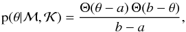 (A.2)where Θ(·),a, and
b are the Heaviside step function, the lower and the upper prior
bounds. Here, we note that the frequentist approach, lacking an explicit definition
of the prior, corresponds to the implicit assumption of a uniform prior for all
parameters.
(A.2)where Θ(·),a, and
b are the Heaviside step function, the lower and the upper prior
bounds. Here, we note that the frequentist approach, lacking an explicit definition
of the prior, corresponds to the implicit assumption of a uniform prior for all
parameters. -
A positive scale parameter, which often spans several decades, is characterised by its invariance against a stretch of the coordinate axis by a factor ϕ, i.e.
 (A.3)which is solved by the Jeffreys prior,
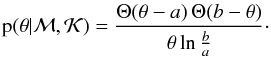 (A.4)That a uniform prior would be
inappropriate for this parameter is also illustrated by the fact that it would
assign higher probabilities to θ lying in a higher decade of
[a,b] than in a lower.
(A.4)That a uniform prior would be
inappropriate for this parameter is also illustrated by the fact that it would
assign higher probabilities to θ lying in a higher decade of
[a,b] than in a lower. -
If the lower prior bound of a scale parameter is zero, e.g. for the RV semi-amplitude K, a modified Jeffreys prior is used. It has the form
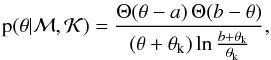 (A.5)where θk is
the knee of the prior. For θ ≪ θk, this
prior is approximately uniform, while it approaches a Jeffreys prior for
θ ≫ θk.
(A.5)where θk is
the knee of the prior. For θ ≪ θk, this
prior is approximately uniform, while it approaches a Jeffreys prior for
θ ≫ θk.
Appendix B: Numerical posterior summaries
The following tables list the numerical values of several posterior summaries. Those in Tables B.1 and B.2 are derived from the marginal posteriors (Fig. 5), while the correlation coefficients in Table B.3 reflect linear relations between parameters and, in this respect, can be regarded as summaries of the joint marginal posteriors (Fig. 6).
Compared to the underlying densities, all of these summaries are incomplete. Still, they are useful e.g. for the calculation of model functions or comparison with literature results.
Pearson correlation coefficients of pairs of parameters.
All Tables
All Figures
|
Fig. 1 Definition of the angles ω⋆,i,Ω. a) From S1 to S2, the star and its sense of rotation about the CM are indicated; the dotted line marks the major axis of the orbital ellipse. b) From S2 to S3, the observer and line of sight are indicated. c) From S3 to S4, the positive x4-axis points northward along the meridian of the CM. |
| In the text | |
|
Fig. 2 Pass A: marginal posteriors of RV amplitudes K1 (top, solid line), K2 (top, dashed line) and offset V (bottom), all plotted over the approximate range of the corresponding 99% HPDI. |
| In the text | |
|
Fig. 3 Pass B: marginal posterior of orbital frequency f, plotted over the range of the corresponding 99% HPDI. This is a Bayesian analogon to the frequentist periodogram. |
| In the text | |
|
Fig. 4 Pass C: marginal posteriors of the argument of periapsis ω2 (solid line) and position angle of the ascending node Ω (dashed line), plotted over the approximate range of the corresponding 99% HPDIs. Triangles indicate the positions of small local maxima located approximately ± π from the corresponding marginal modes. |
| In the text | |
|
Fig. 5 Marginal posteriors of parameters e,f,χ,ω2,i,Ω,ϖ,V,K1,K2 (see also Table 1) and derived quantities P,T,d,ρ,Kalt,1,Kalt,2,m1,m2,a1,a2,arel (Table 2) with marginal-posterior medians (dotted line) and 68.27% HPDIs (dashed lines), from the final pass. Abscissae ranges are identical with the corresponding 95% HPDIs. Ordinate values were omitted but follow from normalisation. Open triangles on the upper abscissae indicate the MAP estimates. Open circles on the lower abscissae bound the confidence intervals given by or derived from Prevot (1961), while open triangles refer to the intervals of Hummel et al. (1998). Some of these literature estimates are not plotted because they are outside the abscissa range; for f and χ, no literature uncertainty estimate is available. For derivations and numerical values, see Tables B.1 and B.2. |
| In the text | |
|
Fig. 6 Two-parameter joint marginal posterior
densities |
| In the text | |
|
Fig. 7 AM and RV data and models calculated with the MAP parameter estimates (Table B.1). a) AM data (uncertainty ellipses, solid lines), model (large ellipse, solid line) and residual vectors (dashed lines). b) Residual AM error ellipses. c) RV data and model for primary (normal error bars, solid line) and secondary (hourglass-shaped error bars, dotted line). The horizontal dashed line indicates the RV offset V. RV residuals are presented in Fig. 8. |
| In the text | |
|
Fig. 8 All data types: from top to bottom: AM data and model (δ coordinate); AM residuals Δδ; AM data and model (αcosδ coordinate); AM residuals Δ(αcosδ); RV data and model v (primary: solid line, secondary: dotted line, RV offset V: horizontal dashed line); RV residuals Δv (primary: normal error bars, secondary: dashed error bars, model: dashed line). AM error bars are defined as the sides of the smallest rectangle orientated along the coordinate axes and containing the respective error ellipse. Abscissa values are mean anomalies M (Eq. (26)), i.e. times folded with respect to the MAP estimates of the time of periapsis T and period P. |
| In the text | |
|
Fig. 9 Distribution of normalised residuals of AM data (long-dashed line), RV data
(short-dashed) and all data (solid), along with the standard normal
distribution |
| In the text | |
Current usage metrics show cumulative count of Article Views (full-text article views including HTML views, PDF and ePub downloads, according to the available data) and Abstracts Views on Vision4Press platform.
Data correspond to usage on the plateform after 2015. The current usage metrics is available 48-96 hours after online publication and is updated daily on week days.
Initial download of the metrics may take a while.