| Issue |
A&A
Volume 544, August 2012
|
|
|---|---|---|
| Article Number | A83 | |
| Number of page(s) | 11 | |
| Section | Cosmology (including clusters of galaxies) | |
| DOI | https://doi.org/10.1051/0004-6361/201118485 | |
| Published online | 01 August 2012 | |
Domain of validity for pseudo-elliptical NFW lens models
Mass distribution, mapping to elliptical models, and arc cross section
1 Instituto de Cosmologia, Relatividade e Astrofísica – ICRA, Centro Brasileiro de Pesquisas Físicas, Rua Dr. Xavier Sigaud 150, CEP 22290-180, Rio de Janeiro, RJ, Brazil
e-mail: This email address is being protected from spambots. You need JavaScript enabled to view it.
2 Laboratório Interinstitucional de e-Astronomia – LIneA, Rua Gal. José Cristino 77, CEP 20921-400, Rio de Janeiro, RJ, Brazil
Received: 18 November 2011
Accepted: 4 June 2012
Abstract
Context. Owing to their computational simplicity, models with elliptical potentials (pseudo-elliptical) are often used in gravitational lensing applications, in particular for mass modeling using arcs and for arc statistics. However, these models generally lead to negative mass distributions in some regions and to dumbbell-shaped surface density contours for high ellipticities.
Aims. We revisit the physical limitations of the pseudo-elliptical Navarro-Frenk-White (PNFW) model, focusing on the behavior of the mass distribution close to the tangential critical curve, where tangential arcs are expected to be formed. We investigate the shape of the mass distribution on this region and the presence of negative convergence. We obtain a mapping from the PNFW to the NFW model with elliptical mass distribution (ENFW). We compare the arc cross section for both models, aiming to determine a domain of validity for the PNFW model in terms of its mass distribution and for the cross section.
Methods. We defined a figure of merit to i) measure the deviation of the iso-convergence contours of the PNFW model to an elliptical shape, ii) assigned an ellipticity εΣ to these contours, iii) defined a corresponding iso-convergence contour for the ENFW model. We computed the arc cross section using the “infinitesimal circular source approximation”.
Results. We extend previous work by investigating the shape of the mass distribution of the PNFW model for a broad range of the potential ellipticity parameter ε and characteristic convergence Ks. We show that the maximum value of ε to avoid dumbbell-shaped mass distributions is explicitly dependent on Ks, with higher ellipticities (ε ≃ 0.5, i.e., εΣ ≃ 0.65) allowed for small Ks. We determine a relation between the ellipticity of the mass distribution εΣ and ε valid for any ellipticity. We also derive the relation of characteristic convergences, obtaining a complete mapping from PNFW to ENFW models, and provide fitting formulae for connecting the parameters of both models. Using this mapping, the cross sections for both models are compared, setting additional constraints on the parameter space of the PNFW model such that it reproduces the ENFW results. We also find that the negative convergence regions occur far from the arc formation region and should therefore not be a problem for studies with gravitational arcs.
Conclusions. We conclude that the PNFW model is well-suited to model an elliptical mass distribution on a larger ε–Ks parameter space than previously expected. However, if we require the PNFW model to reproduce the arc cross section of the ENFW well, the ellipticity is more restricted, particularly for low Ks. The determination of a domain of validity for the PNFW model and the mapping to ENFW models could have implications for the use of PNFW models for the inverse modeling of lenses and for fast arc simulations, for example.
Key words: gravitational lensing: strong / galaxies: clusters: general / galaxies: halos / dark matter
© ESO, 2012
1. Introduction
Gravitational arcs are powerful probes of the mass distribution in galaxies (Koopmans et al. 2009; Barnabè et al. 2011; Suyu et al. 2012) and galaxy clusters (Kovner 1989; Miralda-Escudé 1993a; Hattori et al. 1997) and can be used to constrain cosmological models (Bartelmann et al. 1998; Oguri et al 2001; Golse et al. 2002; Bartelmann et al. 2003; Jullo et al. 2010). The main techniques employed to extract information from gravitational arcs have been arc statistics (i.e. counting the number of arcs in lens samples, Wu & Hammer 1993; Grossman &Saha 1994; Bartelmann & Weiss 1994) and inverse modeling (i.e. “deprojecting” the arcs in individual lens systems to determine the lens and the source, Kneib et al. 1993; Keeton 2001; Golse et al. 2002; Wayth & Webster 2006; Jullo et al. 2007, 2010). The first requires large samples of arcs while the second needs detailed information on the lensing systems, typically imaging from space and lens and source redshifts.
These applications have triggered arc searches in surveys covering large areas (Gladders et al. 2003; Estrada et al. 2007; Cabanac et al. 2007; Kneib et al. 2010; More et al. 2011; Belokurov et al. 2009; Kubo et al. 2010), in large spectrocospic surveys (Bolton et al. 2008; Brownstein et al. 2012), and in surveys targeting known clusters (Luppino et al. 1999; Zaritsky & Gonzalez 2003; Smith et al. 2005; Hennawi et al. 2008; Makler et al. 2010; Richard et al. 2010b; Kausch et al. 2010; Furlanetto et al. 2012). Upcoming wide field imaging surveys, such as the Dark Energy Survey (Abbott et al. 2005; Annis et al. 2005) and the Large Synoptic Survey Telescope (Stubbs et al. 2004; Ivezic et al. 2008), will lead to the identification of larger samples of arcs in thousands of galaxies and galaxy clusters, well suited for arc statistics. Moreover, deep observations from space combined with massive spectroscopy have been obtained for a limited number of clusters and were used for detailed mass modeling (see, e.g., Broadhurst et al. 2005; Richard et al. 2010a; Jullo et al. 2010).
The simplest models that can account for some observed properties of arcs (multiplicity, relative positions, morphology) are built from axial models by introducing an ellipticity either on the mass distribution (elliptical models, Schramm 1990; Barkana 1998; Keeton 2001; Oguri et al. 2003) or on the lensing potential (pseudo-ellitpical models, Blandford & Kochanek 1987; Kassiola & Kovner 1993; Kneib 2002). Most parametric analyses of arcs, both for the inverse modeling (Jullo et al. 2007) and for arc statistics (Oguri 2002; Oguri et al. 2003), involve one or more elliptical/pseudo-elliptical models (adding, in some cases, external shear and substructures).
Elliptical models, whose surface density is constant over ellipses, are more realistic than pseudo-elliptical ones. For example, elliptical models are motivated by the results of N-body simulations, which show that dark matter halos are triaxial (Jing & Suto 2002; Macciò et al. 2007), such that their overall mass distribution can be modeled at first order by ellipsoids, whose surface density contours are elliptical. In contrast, the surface density of pseudo-elliptical models generally has a pathological behavior, exhibiting regions where it takes negative values (Blandford & Kochanek 1987) and presenting a “dumbbell” (or “peanut”) shape for high ellipticities (Kovner 1989; Schneider et al. 1992; Kassiola & Kovner 1993), which does not represent the mass distribution of most physical systems.
On the other hand, pseudo-elliptical models provide simple analytic solutions for some lensing quantities, allowing for fast numerical methods to be implemented, whereas elliptical models require the computation of integrals, which are more demanding numerically (Schramm 1990; Keeton 2001). Therefore, studies that require numerous evaluations of the lensing quantities often employ pseudo-elliptical models. For example, several studies using arc simulations have used these models (Oguri 2002; Meneghetti et al. 2003, 2007). Popular codes for lens inversion (Golse et al. 2002; Wayth & Webster 2006; Jullo et al. 2007) are implemented using this type of model, too.
It is therefore relevant to determine a “domain of validity” for pseudo-elliptical models such that the negative convergence appears far from the arc-forming region and the shape of their mass distribution is closer to elliptical. The determination of such a validity region could be useful, for example, to evaluate if a set of model parameters derived from the inversion of a system with arcs using the pseudo-elliptical Navarro-Frenk-White (PNFW) model is physically acceptable. Even for methods that use the elliptical model (ENFW) for lens inversion (Keeton 2001; Suyu et al. 2012), the PNFW could be useful, within its domain of validity, for a faster coarser probing of the parameter space that would subsequently need to be refined with the elliptical model.
Once a pseudo-elliptical model is found to be acceptable, it is nevertheless necessary to provide a correspondence to an elliptical model. This would be necessary, for example, to compare results derived from the mass modeling using observed arcs with theoretical predictions. We therefore need to establish a mapping among the parameters of the two models. This mapping could also be used to replace an elliptic model by its corresponding pseudo-elliptic in lensing simulations.
In this paper we focus on the widely used PNFW model and investigate its domain of validity as well as the mapping to the corresponding ENFW. To test the equivalence among the two models we compute the cross section for arc formation, from which we obtain additional constraints on the model parameters.
The outline of this paper is as follows: in Sect. 2 we briefly review the PNFW lens model, introducing the conventions and parameter ranges to be used throughout this work. In Sect. 3 we discuss the region of arc formation and derive physical limits of the PNFW mass distribution in this region. In Sect. 4 we consider two ways for assigning an ellipticity to the PNFW surface density. In Sect. 5 we obtain a mapping from the PNFW to the ENFW models. In Sect. 6 we compare the arc cross sections of the two models using the mapping relations. In Sect. 7 we present the summary and concluding remarks. In Appendix A we present useful relations to derive some lensing functions for pseudo-elliptical models. In Appendix B we provide fitting formulae for the limits on the mass distribution of the PNFW model and for the mapping to the ENFW.
2. The pseudo-elliptical NFW lens model
2.1. Circular NFW lens model
From N-body simulations Navarro, Frenk & White (NFW) found that the radial (i.e. angle-averaged) density profile of dark matter haloes approximately follows the universal function (Navarro et al. 1996, 1997) 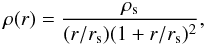 (1)where rs is the scale radius and ρs is the characteristic density of the halo. This profile has been widely used to represent the dark matter mass distribution galaxy to cluster scales and will be employed throughout this work.
From the density profile (1), defining the dimensionless Cartesian coordinates in the lens plane1, x = ξ/rs, the convergence, deflection angle, shear, and lensing potential are given by (Bartelmann 1996): 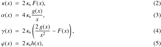 where the functions F(x), g(x) and h(x) are defined in Golse & Kneib (2002, hereafter GK02) and the characteristic convergence, κs, is given by
  (6)with the critical surface mass density
  (7)where DOL, DLS and DOS are the angular-diameter distances between the observer and lens (at redshift zL), lens and source (at redshift zS), and observer and source, respectively (Schneider et al. 1992; Mollerach & Roulet 2002).
Notice that with the choice of dimensionless coordinates x, the lensing functions are independent of rs. Naturally, dimensional quantities have to be scaled accordingly to recover their physical units. For example, angular quantities have to be multiplied by rs/DOL to be in radians.
2.2. Pseudo-elliptical models
To construct “elliptical models” from a given radial density profile, the radial coordinate x is replaced by  (8)such that the ellipticity is given by
  (9)where we assume that a2 > a1, such that the major axis of the ellipse is along x1.
This substitution can be performed on the projected mass distribution, κ(x) → κ(xε), leading to elliptical mass distributions (Bourassa et al. 1973; Bourassa & Kantowski 1975; Bray 1984). An alternative is to construct pseudo-elliptical models, by making the substitution in the lensing potential, ϕ(x) → ϕ(xε), which leads to simple analytic expressions for the lensing functions (GK02; Kassiola & Kovner 1993; Oguri 2002; Jullo et al. 2007). In particular the convergence and the components of the shear are given by (see Appendix A) ![Mathematical equation: \begin{eqnarray} &&\kappa_\varepsilon(\vec{x})=\mathcal{A}\,\kappa(x_\varepsilon) -\mathcal{B}\,\gamma(x_\varepsilon)\cos{2\phi_\varepsilon} \label{kappa_pnfw},\\[2.5mm] &&\gamma_{1\varepsilon}(\vec{x}) = \mathcal{B}\,\kappa(x_\varepsilon)-\mathcal{A}\, \gamma(x_\varepsilon)\cos{2\phi_\varepsilon}, \\[2.5mm] &&\gamma_{2\varepsilon}(\vec{x}) = -\sqrt{\mathcal{A}^2-\mathcal{B}^2}\, \gamma(x_\varepsilon)\sin{ 2\phi_\varepsilon},\\[2.5mm] &&\gamma_\varepsilon^2(\vec{x}) = \mathcal{A}^2\gamma^2(x_\varepsilon)-2\mathcal{A}\, \mathcal {B}\, \kappa(x_\varepsilon)\gamma(x_\varepsilon)\cos{2\phi_\varepsilon} \nonumber \\[2.5mm] & & \phantom{\gamma_\varepsilon^2(\vec{x})~~~~~} +\mathcal{B}^2\left[\kappa^2(x_\varepsilon)-\sin^2{2\phi_\varepsilon} \gamma^2(x_\varepsilon) \right]\label{gamma_pnfw}, \end{eqnarray}](/articles/aa/full_html/2012/08/aa18485-11/aa18485-11-eq32.png) \arraycolsep1.75ptwhere
\arraycolsep1.75ptwhere  ,
,  , and κ(xε) and γ(xε) are the convergence and shear of a circular model evaluated at xε, respectively.
The PNFW model is obtained by introducing the ellipticity on the NFW lens potential (Eq. (5)), where we denote the characteristic convergence (Eq. (6)) by  .
.
In this paper we adopt the convention (Blandford & Kochanek 1987; GK02)  (14)such that the ellipticity of the lensing potential (Eq. (9)) is given by
  (15)and the ellipticity parameter ε is defined in the range 0 ≤ ε < 1.
Using this convention, Eqs. (10) and (13) yield Eqs. (17) and (19) of GK022. Another common choice of parameterization is a1 = 1/(1 − ε), a2 = 1 − ε. In this case the ellipticity of the potential is simply given by εϕ = ε and Eqs. (10)–(13) yield the same expressions for the lensing functions as, for example, in Lima et al. (2010)3.
To obtain the maximum value of to be used in this paper we considered the most extreme lensing systems expected in nature, with4M200 = 4 × 10¹⁵ h-1 M⊙, zL = 1.6, zS = 7 (Oguri & Blandford 2009). The values of rs were obtained from the distribution of the concentration parameter c = r200/rs, p(c | M,z = 0), derived from N-body simulations by Neto et al. (2007) with redshift scaling given in Macciò et al. (2008). From M200, c, zL, and zS we obtained the characteristic convergence by applying the relations for the spherical NFW model (Eqs. (1), (5), and (7), see, e.g., Caminha et al., in prep.), where we chose the ΛCDM matter and cosmological constant density parameters as Ωm = 0.3 and ΩΛ = 0.7, respectively. We generated many realizations of the c–M200 relation, converted them to characteristic convergence, and took the 95% upper limit of the derived distribution as its maximum value, which leads to  . This sets an inclusive upper limit for , at least within the ΛCDM framework.
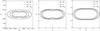 |
Fig. 1 Critical curve (Rλ = ∞), curves of constant distortion (Rλ = ± Rth) and κε contours associated to each Rλ curve (solid lines) for Rth = 10 and |


3. Physical limits of the PNFW mass distribution
We focused on the mass distribution in the vicinity of the region of tangential arc5 formation. The arcs are usually defined as images with length-to-width ratio L/W above a given threshold Rth. For infinitesimal circular sources this ratio can be determined from the radial and tangential eigenvalues of the Jacobian matrix of the lens mapping, λr and λt, respectively (Wu & Hammer 1993; Bartelmann & Weiss 1994; Hamana & Futamase 1997):  (16)where Rλ: = λr/λt, with λr = 1 − κ + γ and λt = 1 − κ − γ.
Fixing a value for Rth determines a region limited by the curves Rλ = ± Rth (constant distortion curves), where gravitational arcs are expected to be formed. Although condition (16) does not hold for images of sources crossing the tangential caustic (merger arcs, Rozo et al. 2008; Ferreira 2010), nor for large or noncircular sources, the curves defined above still provide a typical scale for the region of arc formation. A common choice for the threshold is Rth = 10, which we adopted in this work (unless explicitly stated otherwise). The tangential critical curve is given by the condition Rλ = ∞. In Fig. 1 these curves are shown for a few combinations of and ε.
Once a domain for arc formation has been established, we need to associate to this region iso-convergence contours, denoted by κε contours, which define the shape of the mass distribution. We chose to match the κε contours to the Rλ = ± Rth curves at the major axis (x2 = 0), since most arcs are expected to be formed close to this region (see, e.g., Dalal et al. 2004; Comerford et al. 2006; Meneghetti et al. 2007; More et al. 2011). This definition is illustrated in Fig. 1, where distortion curves and their associated iso-convergence contours are shown. We will use this choice throughout this paper and refer to the κε contour by the value of Rλ associated to it.
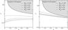 |
Fig. 2 Negative convergence of the PNFW model. Solid lines show the intersection of κε = 0 contours with x2 axis. Other lines correspond to the intersection of the iso-convergence contours associated to Rλ = Rth curves with the x2 axis. Left panel: κs = 0.1. Right panel: κs = 1.5. |
A fundamental problem of pseudo-elliptical models is the presence of regions with negative mass distribution (Kassiola & Kovner 1993). For the PNFW model parameterized as in Eq. (14), negative κε contours form lobes oriented along the x2 axis. These regions occur far from the lens center and for any ε > 0. The κε = 0 contours are independent of and the nearest point to the region of tangential arc formation is located on the x2 axis. For example, in Fig. 1, for ε = 0.3,0.35, and 0.45, negative values of κε arise at x2 = ± 10.5,7.3 and 4.3, respectively, well outside the range of these plots.
We have verified that the κε = 0 contours do not intersect the iso-convergence contours associated to the | Rλ | = Rth curves in the whole ε and range, as can be seen in Fig. 2. As expected, the negative convergence lobes approach the Rλ = const. curves as the ellipticity increases, but never intersects these regions, even down to Rth = 1.25. The lower the characteristic convergence, the farther is the negative convergence region from the arc formation region. Therefore, the formation of tangential arcs occurs far from the κε < 0 regions, and can be ignored in the context of this paper.
Now we turn to the shape of the κε contours. Given the chosen orientation of the major axis, for contours that are close to elliptical, the maximum value of x2 ( ) is located at x1 = 0. On the other hand, for dumbbell-shaped contours is located at x1 ≠ 0. This simple property can be used to determine the maximum value of ε (εmax) such that for ε > εmax a dumbbell-shape emerges. This is shown schematically in Fig. 3. For a given , we started with a low value of ε and computed for the κε contours associated to each Rλ curve. As the ellipticity parameter is increased, εmax is attained when the point corresponding to starts to be located at x1 ≠ 0. Repeating this procedure for any value of and Rλ leads to the function
  .
.
We found that this function is weakly dependent on Rλ. For example, the absolute difference  is at most 0.03 for Rth = 4, corresponding to a fractional difference of about 10%, in the whole range. This maximum difference decreases to 0.01 for Rth = 10. Thus, it is sufficient to define
 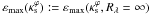 in the arc formation region. This function is shown in Fig. 4. Clearly εmax depends on , decreasing for high characteristic convergences. For low values of , εmax converges to 0.5. In Appendix B.1 we provide a best-fitting function to
  , which could be useful, for example, to check if a given solution from inverse modeling has a physically meaningful mass distribution. The limits on the shape of the iso-convergence contours will be revisited in the next section by measuring the deviation with respect to an elliptical shape.
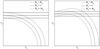 |
Fig. 3 Sketch of the method for determining the maximum value of ε to avoid dumbell-shaped κε contours associated to the Rλ = const. curves. Left panel: shape of the iso-convergence contours for ε < εmax. Right panel: shape of the iso-convergence contours for ε > εmax. |
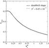 |
Fig. 4 Maximum value of the ellipticity to avoid dumbbell-shaped mass distributions in the region close to the Rλ = ∞ contour as a function of |

4. Ellipticity of the PNFW mass distribution
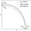 |
Fig. 5 Illustration of the methods used to associate the PNFW mass distribution to elliptical contours. In the GK method, aGK and bGK correspond to the semi-major and semi-minor axes of the ellipse (dashed line) passing through the intersection of the iso-convergence contour (solid line) with the x1 and x2 axes. In the EF method, aEF and bEF correspond to the semi-major and semi-minor axes of the best-fitting ellipse (dash-dotted line) obtained by minimizing Eq. (18). |
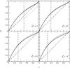 |
Fig. 6 Ellipticity of the PNFW mass distribution εΣ from the elliptical fit ( |

We adopted two procedures to associate an ellipticity εΣ to each κε contour and to measure its deviation from an elliptical shape. In the first, we followed GK02 and define the semi-major axis aGK and semi-minor axis bGK as the intersections of the κε contour with the x1 and x2 axes, respectively (see Fig. 5), such that the ellipticity is 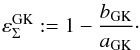 (17)The second procedure is to fit the κε contour by an ellipse. For this sake we introduce a figure-of-merit that represents the mean weighted squared fractional radial difference between the contour and the ellipse
 ![Mathematical equation: \begin{equation} \mathcal{D}^ 2 :=\frac{\sum_{i=1}^N\,w_i[r(\phi_{i})-r_\Sigma(\phi_{i}) ]^2 } {\sum_{i=1}^N w_i\, r^2(\phi_{i})}, \label{gof-ef} \end{equation}](/articles/aa/full_html/2012/08/aa18485-11/aa18485-11-eq119.png) (18)where N is the number of points on the κε contour, φi is their polar angle, wi = φi − φi − 1 is a weight accounting for a possible non-uniform distribution of φi, r(φi) is the radial coordinate of the κε contour and rΣ(φi) is the radial coordinate of the ellipse, given by
(18)where N is the number of points on the κε contour, φi is their polar angle, wi = φi − φi − 1 is a weight accounting for a possible non-uniform distribution of φi, r(φi) is the radial coordinate of the κε contour and rΣ(φi) is the radial coordinate of the ellipse, given by ![Mathematical equation: \begin{equation} r_\Sigma=\left[\left(\frac{\cos{\phi}}{a}\right)^2+ \left(\frac{\sin{\phi}}{b}\right)^2\right]^{-1/2}, \label{first-elipse} \end{equation}](/articles/aa/full_html/2012/08/aa18485-11/aa18485-11-eq124.png) (19)where a and b are the semi major and minor axes, respectively. The form of
(19)where a and b are the semi major and minor axes, respectively. The form of  in Eq. (18) was chosen to be scale-invariant and independent of the discretization6. Owing to the symmetry of the κε contour, it is sufficient to compute in the first quadrant of the lens plane.
The best-fitting ellipse is found by minimizing , for which we used the MINUIT code (James 1998). The resulting best-fitting values from this elliptical fit (EF) method, aEF and bEF, yield the ellipticity 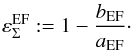 (20)When the iso-convergence contours are close to elliptical, we expect the results from both methods to be very similar. However, differences could emerge for high values of ε, especially in the dumbbell-shape regime. Another difference that will be discussed in Sect. 5 arises when assigning a κε contour to the derived ellipse.
We may associate an ellipticity to the iso-convergence contours related to each distortion curve. However, the functions  are weakly dependent on Rλ close to the arc formation region. For example, the absolute differences
  are at most 0.01 for Rth = 10 and 0.02 for Rth = 4. Therefore, we chose the ellipticity associated to the convergence at the critical curve (Rλ = ∞) as the ellipticity in the arc formation region. In Fig. 6 the resulting values for
  (dashed lines) and
  (solid lines) are shown as a function of ε, for
  , 1.0, and 1.5.
As expected, the two ellipticity measures agree very well for low values of ε. For example, for ε = 0.25,  is at most 0.03 on the whole range. As can be seen in Fig. 6, although the behavior of the two functions is qualitatively very similar in the whole ellipticity range, noticeable differences appear precisely for the values of ε (shown in Fig. 4) close to where the dumbbell-shape arises.
The minimum value of the figure-of-merit (18)  can be used as a goodness of fit and hence as an estimator of the departure from the elliptical shape. By setting a threshold on a maximum value of ε can be determined, for each , such that does not exceed this threshold, ensuring a small deviation from the elliptical shape. In particular, setting this threshold at 4.5 × 10⁻⁴ avoids the dumbbell-shaped mass distribution, as shown in Fig. 4. Thus, a small deviation from the elliptical shape is deeply connected to the avoidance of dumbbell shapes. Both conditions impose similar restrictions on the ellipticity and imply that the PNFW could be used to model the mass distribution in the region of arc formation for ε below the limits given in Fig. 4 and Eq. (B.1).
The validity of the PNFW to represent elliptical mass distributions was also investigated in GK02. They considered a single value of the characteristic convergence and investigated the shape of the mass distribution as a function of the distance of the κε contour to the lens center. They provide a fitting function for εΣ as a function of  and ε, valid for ε < 0.25. Their lensing potential depth is expressed in terms of a characteristic velocity vc, connected to the NFW profile parameters by (Golse et al. 2002)
  (21)Using the values in GK02 (vc = 2000 km s-1, rs = 150 kpc, zL = 0.3, and zS = 1), assuming Ωm = 0.3, ΩΛ = 0.7, and H0 = 65 km s-1 Mpc-1, and using Eqs. (6) and (7) yields
  . Our results for
  reproduce their fit to within 2% down to its limit of validity.
On the other hand, by exploring a large interval of  , we find that higher values of ε may be allowed, at least in the region of arc formation. In particular, values as high as ε ≃ 0.5 (corresponding to εΣ ≃ 0.65, see Fig. 6) are permitted for low . It is therefore useful to provide a fit that is valid beyond ε = 0.25 and includes the dependence of the ellipticity with . Such a fitting function for
  is shown in Appendix B.2, which is valid in the whole range of ε and the range of considered in this paper.
5. Mapping among the PNFW and ENFW models
The ENFW model is constructed by replacing κ(x) in Eq. (2) by κ(xεΣ) (see Sect. 2.2), where xεΣ is chosen as (Caminha et al., in prep.)  (22)such that εΣ is the ellitpicity of the mass distribution. In this case we denote the NFW characteristic convergence by
  .
.
We constructed a mapping among the PNFW and ENFW models such that their mass distribution is similar on the arc formation region. In other words, for each pair (, ε) we associated a corresponding pair of the ENFW model parameters (, εΣ), where is the characteristic convergence of the associated ENFW model. The ellipticity of the ENFW mass distribution εΣ is simply given by the ellipticity associated to the κε contours, as discussed in Sect. 4, with approximate expressions given in Appendix B.2.
The determination of is numerically more complex and involves an ambiguity on how to perform the matching among models. We have chosen to perform the matching at aEF, i.e., at the intersection of the best-fitting ellipse to the κε contour associated to a given Rλ = const. curve with the x1 axis. We have considered two possibilities: i) matching the value of the ENFW convergence at aEF with the PNFW convergence associated to the Rλ = const. curve, ii) matching the position of Rλ = const. curve of the ENFW model, i.e. such that it intersects the x1 axis at aEF. For any pair (, ε) we fixed the ellipticity of the ENFW model as  and obtained following the two procedures above.
The two possibilities described above yield very similar values for down to high ellipticites. For example, taking as reference the κε associated to the critical curve (i.e. to Rλ = ∞), the maximum difference of among the two procedures for  and ε = 0.8 is 3% and this difference decreases substantially for lower ellipticities and
  . On the other hand, if instead of using aEF as reference position for the association of we use aGK, the results are still very similar for
  , but may differ substantially for higher ellipticities.
As described above, convergences can be matched for κε contours associated to any Rλ curve. We verified that the derived characteristic convergence is almost constant in the region of tangential arc formation. Indeed, the absolute differences  are at most 0.005 (0.01), for
  and 0.01 (0.03), for
  , with Rth = 10 (Rth = 4), and ε < 0.6. Therefore, as in the εΣ case, we chose the characteristic convergence in the region of arc formation as the value of
  calculated at the intersection of Rλ = ∞ with the x1 axis. As will be discussed in Sect. 6, we chose method (ii) to make the association between the two models.
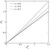 |
Fig. 7 Relation among the characteristic convergences of the PNFW and ENFW models for some values of the parameter ε calculated at the tangential critical curve (Rλ = ∞) at x2 = 0. The solid line shows the |
In Fig. 7 we show as a function of for some values of ε. As expected, for ε = 0 we have  , but this equality does not hold for non-zero ellipticities. In particular, is always larger than its corresponding , and the difference between them increases with ε. In Appendix B.3 we provide a fitting function for .
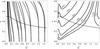 |
Fig. 8 Comparison between arc cross sections. Left panel: contours of constant arc cross section in terms of the PNFW parameters. Solid lines correspond to |

6. Comparison of the arc cross section
The efficiency of a lens to produce arcs is quantified by the arc cross section  , which is defined as the area in the source plane that generates images with L/W ≥ Rth, weighted by the multiplicity of the images (i.e. multiply imaged regions are counted multiple times, see e.g., Meneghetti et al. 2003). The computation of the arc cross section usually requires extensive arc simulations, which are computationally expensive (Miralda-Escudé 1993b; Bartelmann & Weiss 1994; Meneghetti et al. 2001, 2003; Oguri et al. 2003). However, in the infinitesimal circular source approximation, Eq. (16), the cross section can be obtained directly from the local mapping from lens to source plane. In this case is easily computed in the lens plane (in dimensionless coordinates) by (see, e.g., Fedeli et al. 2006; Caminha et al., in prep.)
 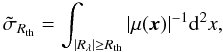 (23)where
  is the magnification and the integral is performed over a region with local distortion above the given threshold (i.e., the arc formation region introduced in Sect. 3 and used in the preceding sections). Since the mapping between the PNFW and ENFW models was constructed in that region, the cross section is well suited to check if this mapping, obtained from matching the mass distribution, also holds for other lensing quantities, in this case the magnification.
If the PNFW can be used to replace the ENFW in some applications (for example, arc statistics), we would expect the predictions for to be similar for both models, at least in the region where the PNFW provides an adequate description for the mass distribution. On the other hand, if the predictions do not match in this region, they can be used to set additional constraints on the PNFW model.
To compare the cross section for both models we defined a regular grid in the ( ) parameter space and mapped each point to (
 ) using the procedures described in Sect. 5. The cross sections
  and
and  were computed for each set of parameters from Eq. (23) using the expressions for λr(x) and λt(x) of the corresponding model. The computation for the ENFW model was taken from Caminha et al. (in prep.). The result for both cross sections is shown in the left panel of Fig. 8 where contours of constant are displayed. Visually, the arc cross sections of both models are similar in the region ε < εmax.
To quantify the difference between and , we computed the relative difference 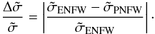 (24)We have computed this fractional difference using the various possibilities for associating ENFW model parameters to PNFW parameters discussed in Sect. 5. Although those definitions generally yield similar values for , the value of
  can vary substantially, since the cross section is very sensitive to κs. Comparing the matches at aEF and aGK, the latter gives a fractional difference at least 50% higher than the former and this difference increases substantially with . The difference between the methods (i) and (ii) is much smaller and is not very sensitive to , but in general procedure (ii) leads to smaller differences in the cross section than method (i). We chose therefore to define the matching among models using method (ii) at aEF and compared the cross sections using this choice.
In the right panel of Fig. 8 the contours of constant relative difference are shown. Our results show that for ε < εmax,  can be as high as 30% for low values of . Thus, even in the region where the ENFW and PNFW mass distributions are similar, there can be substantial deviations on the cross section.
We may combine the constraints from the shape of the mass distribution and by assuming a maximum fractional deviation for the cross section. For example, for a maximum deviation of 10%, the joint constraint leads to a region limited approximately by the lines 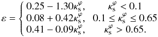 (25)Within this region the PNFW model can reproduce both the local mapping and the mass distribution of the ENFW model.
7. Summary and concluding remarks
Motivated by its potential applications for gravitational arcs, we revisited the PNFW model, seeking to determine domains of validity in terms of the mass distribution and the arc cross section. We have shown that the lensing functions of pseudo-elliptical models have simple analytic expressions (Eqs. (10)–(13)) for any choice of the parameterization of the ellipticity.
We analyzed the PNFW mass distribution, in the “arc formation region” limited by the constant distortion curves (Rλ = ± Rth) by associating κε contours to these curves. We verified that the convergence never takes negative values in this region. Since the results obtained in this work are weakly dependent on Rth, for Rth > 4, we chose the critical curve (Rλ → ∞) to derive the final relations summarized below.
We determined the maximum value of the potential ellipticity parameter, , such as to avoid dumbbell-shaped mass distributions. The results (Fig. 4) enlarge the domain of applicability of the PNFW model to describe the mass distribution, at least in the arc formation region, beyond the commonly adopted value of ε ≃ 0.25, allowing values as high as ε = 0.5 for low values of .
We introduced the figure-of-merit  (Eq. (18)) to quantify the deviation of the κε contours from the elliptical shape. Setting a maximum value for at 4.5 × 10⁻⁴ also avoids dumbbell-shaped mass distribution (Fig. 4), showing that the contours deviate from the elliptical shape on the verge of the emergence of the dumbbell shape.
The function can be used to assign a best-fitting ellipse to the κε contour and hence to obtain an ellipticity εΣ for the mass distribution (EF method). We showed that the ellipticites εΣ obtained from this method are almost identical to the method in GK02, especially for low ellipticities. However, the EF is better suited to assign an iso-convergence contour to the κ contour. Furthermore, using the EF allows one to match between the PNFW and the ENFW models in a way that minimizes the difference between cross sections.
We provided fitting functions for  (Eqs. (B.2), (B.3)), extending the results of GK02, in the arc formation region, for any value of ε and including the dependence on . Going to higher ellipticities is relevant, given that values as high as ε ≃ 0.5 (corresponding to εΣ ≃ 0.65, see Fig. 6) are allowed in the arc formation region.
From N-body simulations, it is found that the probability distribution of the projected ellipticity peaks at about εΣ = 0.5, with only a small fraction of the halos having εΣ > 0.6 (Oguri et al. 2003). Converting  to εΣ we found that values of εΣ > 0.5 are allowed in the whole investigated range of . Therefore, the PNFW would provide a good description of the ENFW mass distribution for most expected values of εΣ.
By associating the iso-convergence contours of the PNFW to the ENFW close to the tangential critical curve, we obtained a relation among characteristic convergences . Fitting functions for this relation are provided in Appendix B.3 (for the case (ii) discussed in Sect. 5). Combined with the relation among ellipticities, this function completes the mapping of the parameters ( ) of the PNFW model to the parameters (
 ) of the ENFW model.
To test the mapping in a practical application we compared the predictions for a quantity that is useful in arc statistics. We computed the arc cross sections for both the PNFW and ENFW models and compared their predictions by matching the model parameters using this mapping. We did not find a direct connection between and εmax (which has a similar shape as a function of as the contours of constant ), although the cross section was computed in the region where the mapping is obtained. In other words, the limits derived from the shape of the mass distribution do not match those from cross section.
We may use this result to set additional constraints on the parameters of the PNFW model, by requiring an agreement with the ENFW for  in addition to the condition
  . This would ensure that the mass distribution as well as the local mapping (represented by the magnification μ) are well reproduced by the PNFW. Approximate limits of this combined restriction, imposing an agreement of about 10% for the cross sections, are given in Eq. (25).
This new restriction should now be tested in other applications, especially with simulations using finite sources, to check if the PNFW and ENFW can be mapped to reproduce the same physical results. This would validate the use of pseudo-elliptical models for simulations and the inverse problem, providing the relation to the associated elliptical model.
In Eq. (1)  , where z is the coordinate on the lens–observer direction and ξ = | ξ | is the coordinate perpendicular to the line-of-sight (lens plane).
After accounting for the known typo, in Eq. (19) of GK02 (cos22φε → sin22φε). We thank the authors for pointing this out on the lenstool code (Jullo et al. 2007) at http://www.oamp.fr/cosmology/lenstool/.
After rotating the lens by π/2 to follow their convention.
Where M200 is defined as the mass contained within a radius r200 enclosing a region with mean density 200 times the critical density of the Universe at zL and h is the Hubble parameter in units of 100 Mpc km-1 s.
Radial arcs are more difficult to observe because they are hidden by the light of the lens, since they are formed in the central region of the lenses and are usually fainter images (Miralda-Escudé 1991; Bartelmann 2003).
A convergence to within about 1% is achieved for N = 100 for the parameter ranges considered here.
Acknowledgments
We thank the anonymous referee for useful comments and suggestions that led to considerable improvements on this manuscript. H. S. Dúmet-Montoya is funded by CNPq (PDJ/162989/2011-3), FAPERJ (“Nota 10” fellowship, E-26/101.784/2010), and the PCI/MCTI program at CBPF (301.860/2011-4). G. B. Caminha is funded by CNPq and CAPES. M. Makler is partially supported by CNPq (grants 312876/2009-2 and 486138/2007-0) and FAPERJ (grant E-26/110.516/2012). We also acknowledge the support of the Laboratório Interinstitucional de e-Astronomia (LIneA) operated jointly by the Centro Brasileiro de Pesquisas Físicas (CBPF), the Laboratório Nacional de Computação Científica (LNCC) and the Observatório Nacional (ON) and funded by the Ministry of Science, Technology and Innovation (MCTI).
References
- Abbott, T., Aldering, G., Annis, J., et al. (The Dark Energy Survey Collaboration) 2005 [arXiv:astro-ph/0510346] [Google Scholar]
- Annis, J., Bridle, S., Castander, F. J., et al. 2005 [arXiv:astro-ph/0510195] [Google Scholar]
- Barkana, R. 1998, ApJ, 502, 531 [NASA ADS] [CrossRef] [Google Scholar]
- Bartelmann, M. 1996, A&A, 313, 697 [NASA ADS] [Google Scholar]
- Bartelmann, M. 2003, in Matter and Energy in Clusters of Galaxies, eds. S. Bowyer, & Chorng-Yuan Hwang, ASP Conf. Proc., 203, 255 [Google Scholar]
- Bartelmann, M., & Weiss, A. 1994, A&A, 287, 1 [NASA ADS] [Google Scholar]
- Bartelmann, M., Huss, A., Colberg, J. M., et al. 1998, A&A, 330, 1 [NASA ADS] [Google Scholar]
- Bartelmann, M., Meneghetti, M., Perrota, F., et al. 2003, A&A, 409, 449 [NASA ADS] [CrossRef] [EDP Sciences] [Google Scholar]
- Barnabè, M., Czoske, O., Koopmans, L. V. E., et al. 2011, MNRAS, 415, 2215 [NASA ADS] [CrossRef] [Google Scholar]
- Blandford, R. D., & Kochanek, C. S. 1987, ApJ, 321, 658 [NASA ADS] [CrossRef] [Google Scholar]
- Belokurov, V., Evans, N. W., Hewett, P. C., et al. 2009, MNRAS, 392, 104 [NASA ADS] [CrossRef] [Google Scholar]
- Bourassa, R. R., Kantowski, R., & Norton, T. D. 1973, ApJ, 185, 747 [NASA ADS] [CrossRef] [Google Scholar]
- Bolton, A. S., Burles, S., Koopmans, L. V. E., et al. 2008, ApJ, 682, 964 [NASA ADS] [CrossRef] [Google Scholar]
- Bourassa, R. R., & Kantowski, R. 1975, ApJ, 195, 13 [NASA ADS] [CrossRef] [Google Scholar]
- Bray, I. 1984, MNRAS, 208, 511 [NASA ADS] [Google Scholar]
- Broadhurst, T., Benítez, N., Coe, D., et al. 2005, ApJ, 621, 53 [NASA ADS] [CrossRef] [Google Scholar]
- Brownstein, J. R., Bolton, A. S., Schlegel, D. J., et al. 2012, ApJ, 744, 41 [NASA ADS] [CrossRef] [Google Scholar]
- Cabanac, R. A., Alard, C., Dantel-Fort, M., et al. 2007, A&A, 461, 813 [NASA ADS] [CrossRef] [EDP Sciences] [Google Scholar]
- Comerford, J. M., Meneghetti, M., Bartelmann, M., et al. 2006, ApJ, 642, 39 [NASA ADS] [CrossRef] [Google Scholar]
- Dalal, N., Holder, G., & Hennawi, J. F. 2004, ApJ, 609, 50 [NASA ADS] [CrossRef] [Google Scholar]
- Estrada, J., Annis, J., Diehl, H. T., et al. 2007, ApJ, 660, 1176 [NASA ADS] [CrossRef] [Google Scholar]
- Fedeli, C., Meneghetti, M., Bartelmann, M., et al. 2006, A&A, 447, 419 [NASA ADS] [CrossRef] [EDP Sciences] [Google Scholar]
- Ferreira, P. 2010, MSc Thesis, Federal University of Rio de Janeiro [Google Scholar]
- Furlanetto, C., Santiago, B. X., Makler, M., et al. 2012, MNRAS submitted [Google Scholar]
- Gladders, M. D., Hoekstra, H., Yee, H. K. C., et al. 2003, ApJ, 593, 48 [NASA ADS] [CrossRef] [Google Scholar]
- Golse, G., & Kneib, J.-P. 2002, A&A, 390, 821 (GK02) [NASA ADS] [CrossRef] [EDP Sciences] [Google Scholar]
- Golse, G., Kneib, J.-P., & Soucail, G. 2002, A&A, 387, 788 [NASA ADS] [CrossRef] [EDP Sciences] [Google Scholar]
- Grossman, S. A., & Saha, P. 1994, ApJ, 431, 74 [NASA ADS] [CrossRef] [Google Scholar]
- Hamana, T., & Futamase, T. 1997, MNRAS, 286, L7 [NASA ADS] [CrossRef] [Google Scholar]
- Hattori, M., Watanabe, K., & Yamashita, K. 1997, A&A, 319, 764 [NASA ADS] [Google Scholar]
- Hennawi, J. F., Gladders, M. D., Oguri, M., et al. 2008, AJ, 135, 664 [NASA ADS] [CrossRef] [Google Scholar]
- Ivezic, Z., Tyson, J. A., Allsman, R., et al. (the LSST Collaboration) 2008 [arXiv:astro-ph/0805.2366] [Google Scholar]
- James. F. 1998, MINUIT: Function Minimization and Error Analysis, CERN Program Library Long Writeup D506 [Google Scholar]
- Jing, Y. P., & Suto, Y. 2002, ApJ, 574, 538 [NASA ADS] [CrossRef] [Google Scholar]
- Jullo, E., Kneib, J.-P., Limousin, M., et al. 2007, New J. Phys., 9, 447 [Google Scholar]
- Jullo, E., Natarajan, P., Kneib, J.-P., et al. 2010, Science, 329, 924 [NASA ADS] [CrossRef] [PubMed] [Google Scholar]
- Kassiola, A., & Kovner, I. 1993, ApJ, 417, 450 [NASA ADS] [CrossRef] [Google Scholar]
- Kausch, W., Schindler, S., Erben, T., et al. 2010, A&A, 513, A8 [NASA ADS] [CrossRef] [EDP Sciences] [Google Scholar]
- Keeton, C. R. 2001, unpublished [arXiv:astro-ph/0102340] [Google Scholar]
- Kneib, J.-P. 2002, in The Shapes of Galaxies and Their Halos. Proc. of the Yale Cosmology Workshop, ed. P. Natarajan (World Scientific Publishing Co. Pte. Ltd), 50 [Google Scholar]
- Kneib, J.-P., Mellier, Y., Fort, B., et al. 1993, A&A, 273, 367 [NASA ADS] [Google Scholar]
- Kneib, J.-P., Van Waerbeke, L., Makler, M., et al. 2010, CFHT/Megacam High-Resolution Imaging of the SDSS Stripe 82, CFHT projects 10BF023, 10BC022, 10BB009 [Google Scholar]
- Koopmans, L. V. E., Bolton, A., Treu, T., et al. 2009, ApJ, 703, L51 [NASA ADS] [CrossRef] [Google Scholar]
- Kovner, I. 1989, ApJ, 337, 621 [NASA ADS] [CrossRef] [Google Scholar]
- Kubo, J. M., Allam, S. S., Drabek, E., et al. 2010, ApJ, 724, 137 [Google Scholar]
- Lima, M., Jain, B., & Mark, D. 2010, MNRAS, 406, 2352 [NASA ADS] [CrossRef] [Google Scholar]
- Luppino, G. A., Goia, I. M., Hammer, F., et al. 1999, A&A, 136, 117 [Google Scholar]
- Macciò, A. V., Dutton, A. A., van den Bosch, F. C., et al. 2007, MNRAS, 378, 55 [NASA ADS] [CrossRef] [Google Scholar]
- Macciò, A. V., Dutton, A. A., & van den Bosch, F. C. 2008, MNRAS, 391, 1940 [NASA ADS] [CrossRef] [Google Scholar]
- Makler, M., Cypriano, E., Santiago, B., et al. 2010, SOAR Gravitational Arc Survey, SOAR projects SO2008B-015, SO2010B-023 [Google Scholar]
- Meneghetti, M., Yoshida, N., Bartelmann, M., et al. 2001, MNRAS, 325, 435 [NASA ADS] [CrossRef] [Google Scholar]
- Meneghetti, M., Bartelmann, M., & Moscardini, L. 2003, MNRAS, 340, 105 [NASA ADS] [CrossRef] [Google Scholar]
- Meneghetti, M., Bartelmann, M., Jenkins, A., et al. 2007, MNRAS, 381, 171 [NASA ADS] [CrossRef] [Google Scholar]
- Miralda-Escudé, J. 1991, ApJ, 370, 1 [NASA ADS] [CrossRef] [Google Scholar]
- Miralda-Escudé, J. 1993a, ApJ, 403, 497 [NASA ADS] [CrossRef] [Google Scholar]
- Miralda-Escudé, J. 1993b, ApJ, 403, 509 [NASA ADS] [CrossRef] [Google Scholar]
- Mollerach, S., & Roulet, E. 2002, Gravitational Lensing and Microlensing (World Scientific Publishing Co. Pte. Ltd.) [Google Scholar]
- More, A., Cabanac, R., More, S., et al. 2012, ApJ, 749, 38 [Google Scholar]
- Navarro, J. F., Frenk, C. S., & White, S. D. M. 1996, ApJ, 462, 563 [NASA ADS] [CrossRef] [Google Scholar]
- Navarro, J. F., Frenk, C. S., & White, S. D. M. 1997, ApJ, 490, 493 [NASA ADS] [CrossRef] [Google Scholar]
- Neto, A. F., Gao, L., Bett, P., et al. 2007, MNRAS, 381, 1450 [NASA ADS] [CrossRef] [Google Scholar]
- Oguri, M. 2002, ApJ, 573, 51 [NASA ADS] [CrossRef] [Google Scholar]
- Oguri, M., & Blandford, R. D. 2009, MNRAS, 392, 930 [NASA ADS] [CrossRef] [Google Scholar]
- Oguri, M., Taruya, A., & Suto, Y. 2001, ApJ, 559, 572 [NASA ADS] [CrossRef] [Google Scholar]
- Oguri, M., Lee, J., & Suto, Y. 2003, ApJ, 599, 7; erratum 2004, 608,1175 [NASA ADS] [CrossRef] [Google Scholar]
- Richard, J., Kneib, J.-P., Limousin, M., et al. 2010a, MNRAS, 402, L44 [NASA ADS] [CrossRef] [Google Scholar]
- Richard, J., Smith, G. P., Kneib, J.-P., et al. 2010b, MNRAS, 404, 325 [NASA ADS] [Google Scholar]
- Rozo, E., Nagai, D., Keeton, C., et al. 2008, ApJ, 687, 22 [NASA ADS] [CrossRef] [Google Scholar]
- Schneider, P., Elhers, J., & Falco, E. E. 1992, Gravitational lenses (Berlin: Springer-Verlag) [Google Scholar]
- Schramm, T. 1990, A&A, 231, 19 [NASA ADS] [Google Scholar]
- Smith, G. P., Kneib, J.-P., Smail, I., et al. 2005, MNRAS, 359, 417 [NASA ADS] [CrossRef] [Google Scholar]
- Stubbs, C. W., Sweeney, D., Tyson, J. A., et al. 2004, BAAS, 36 [Google Scholar]
- Suyu, S. H., Hensel, S. W., McKean, J. P., et al. 2012, ApJ, 750, 10 [NASA ADS] [CrossRef] [Google Scholar]
- Wayth, R. B., & Webster, R. L. 2006, MNRAS, 372, 1187 [NASA ADS] [CrossRef] [Google Scholar]
- Wu, X. P., & Hammer, F. 1993, MNRAS, 262, 187 [NASA ADS] [CrossRef] [Google Scholar]
- Zaritsky, D., & Gonzalez, A. H. 2003, ApJ, 584, 691 [NASA ADS] [CrossRef] [Google Scholar]
Appendix A: Lensing functions for pseudo-elliptical models
To derive the lensing functions for pseudo-elliptic models, it is useful to introduce the following coordinate transformation: 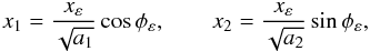 (A.1)where
  and
and  . The Jacobian matrix of this transformation is
 ![Mathematical equation: \appendix \setcounter{section}{1} \begin{eqnarray} \mathcal{J}(\vec{x},\vec{x}_\varepsilon)&=&\left[\!\begin{array}{c c} \frac{1}{\sqrt{{a_{1}}}}\cos{\phi_\varepsilon} &\; -\frac{x_\varepsilon}{\sqrt{{a_{1}}}}\sin{\phi_\varepsilon} \\ \frac{1}{\sqrt{{a_{2}}}}\sin{\phi_\varepsilon} &\; \frac{x_\varepsilon}{\sqrt{{a_{2}}}}\cos{\phi_\varepsilon} \end{array}\!\right]. \label{jacob_transf-vx1-vxe} \end{eqnarray}](/articles/aa/full_html/2012/08/aa18485-11/aa18485-11-eq215.png) (A.2)Since the gradient operator transforms as
(A.2)Since the gradient operator transforms as  , we have
  Using the expressions above, the deflection angle (αε(x) = ∇xϕ(xε)) for an elliptical potential reads (GK02)
  (A.5)where α(xε) is the deflection angle of a circular model evaluated at x = xε.
Taking the partial derivatives of each component of the angle deflection and using Eqs. ((A.3), (A.4)) it is straightforward to obtain ![Mathematical equation: \appendix \setcounter{section}{1} \begin{eqnarray} \partial_{x_1}\alpha_{1}(\vec{x})&=& a_{1}\left[\frac{{\rm d}\alpha(x_\varepsilon)}{{\rm d} x_\varepsilon}\cos^2{\phi_\varepsilon} +\frac{\alpha(x_\varepsilon)}{x_\varepsilon}\sin^2{\phi_\varepsilon}\right], \label{comp_x_elad}\\[1mm] \partial_{x_2}\alpha_{2}(\vec{x})&=& a_{2}\left[\frac{{\rm d}\alpha(x_\varepsilon)}{{\rm d} x_\varepsilon}\sin^2{\phi_\varepsilon} +\frac{\alpha(x_\varepsilon)}{x_\varepsilon}\cos^2{\phi_\varepsilon} \right],\label{comp_y_elad}\\[1mm] \partial_{x_2}\alpha_{1}(\vec{x})&=&\frac{\sqrt{a_{1}a_{2}}}{2} \left[\frac{{\rm d}\alpha(x_\varepsilon)}{{\rm d} x_\varepsilon}-\frac{\alpha(x_\varepsilon)}{x_\varepsilon}\right]\sin{2\phi_\varepsilon}\nonumber \\[1mm] &=& \partial_{x_1}\alpha_{2}(\vec{x}) \label{comp_xy_elad}. \end{eqnarray}](/articles/aa/full_html/2012/08/aa18485-11/aa18485-11-eq222.png) Using the relations for the lensing functions for circular potentials
Using the relations for the lensing functions for circular potentials ![Mathematical equation: \appendix \setcounter{section}{1} \begin{eqnarray} \kappa(x)=\frac{1}{2}\left[\frac{\alpha(x)}{x} + \frac{{\rm d}\alpha(x)}{{\rm d} x}\right], \,\, \gamma(x)=\frac{1}{2}\left[\frac{\alpha(x)}{x}- \frac{{\rm d}\alpha(x)}{{\rm d} x}\right],\label{gamma_circ} \end{eqnarray}](/articles/aa/full_html/2012/08/aa18485-11/aa18485-11-eq223.png) (A.9)it is possible to express Eqs. (A.6)–(A.8) as a function of κ(xε) and γ(xε), i.e.
(A.9)it is possible to express Eqs. (A.6)–(A.8) as a function of κ(xε) and γ(xε), i.e. ![Mathematical equation: \appendix \setcounter{section}{1} \begin{eqnarray} \partial_{x_1}\alpha_{1}(\vec{x})&=& a_{1}\left[\kappa(x_\varepsilon)-\gamma(x_\varepsilon)\cos{2\phi_\varepsilon}\right], \label{comp_x_elad2}\\[1mm] \partial_{x_2}\alpha_{2}(\vec{x})&=& a_{2}\left[\kappa(x_\varepsilon)+\gamma(x_\varepsilon)\cos{2\phi_\varepsilon}\right],\label{comp_y_elad2}\\[1mm] \partial_{x_2}\alpha_{1}(\vec{x})&=&-\sqrt{a_{1}a_{2}}\gamma(x_\varepsilon) \sin{2\phi_\varepsilon}=\partial_{x_1}\alpha_{2}(\vec{x}). \label{comp_xy_elad2} \end{eqnarray}](/articles/aa/full_html/2012/08/aa18485-11/aa18485-11-eq224.png) Applying the usual definitions for the convergence and shear in terms of the deflection angle, we obtain Eqs. ((10)–(13)).
Applying the usual definitions for the convergence and shear in terms of the deflection angle, we obtain Eqs. ((10)–(13)).
Appendix B: Fitting formulae for εmax and for the PNFW-ENFW mapping
B.1. Fitting formula for εmax.
Applying the procedure outlined in Sect. 3, we obtained the maximum value εmax to avoid the dumbbell-shaped mass distribution as a function of . For  we have εmax = 0.5 (corresponding to the plateau in Fig. 4). For higher values of this function is well fitted by a Padé approximant of the form
  (B.1)where a0 = 0.502, a1 = −0.301, a2 = 0.043, a3 = 0.078, a4 = −0.037 and b0 = 0.932, b1 = 0.092, b2 = −0.107, which provides an excellent fit (χ2 < 4 × 10⁻⁶), for values of in the range [0.1,1.5] .
B.2. Fitting formulae for the ellipticity of the mass distribution of the PNFW model
We have verified that the ratio εΣ/ε is well-fitted by a third-order polynomial in ε for the whole range of this parameter,  (B.2)The values of the coefficients ci are obtained from this fit for each in the considered range. These functions are in turn fitted by Padé approximants of the form
  (B.3)where the coefficients dn and em are given in Table B.1.
Results from the regression analysis using the Padé approximant for  .
.
We verified that the combination of (B.2) and (B.3) is indeed a good approximation for the ellipticity of the convergence contours in the region associated to the curves Rλ = ± Rth. For example, the absolute difference  is at most 10-3 in the whole range of ε and .
B.3. Fitting formulae for mapping characteristic convergences
The relation between the characteristic convergence of the PNFW model () and the characteristic convergence of the ENFW model () is fitted by a quadratic function in  (B.4)By construction p0(ε) → 0, p1(ε) → 1, and p2(ε) → 0 as ε → 0.
We divide the regression analysis into two ranges of . For  we choose p0(ε) = 0 and found that p1(ε) and p2(ε) are well-fitted by
  (B.5)with coefficients gn, hn and kn given in Table B.2 (which are valid for ε ≤ 0.8). We check the accuracy of Eq. (B.4) with p1(ε) and p2(ε) given above by computing the χ2 for
  and ε ≤ 0.6, and we found that it is less than 3 × 10⁻⁹ in this range of parameter values.
Results from the regression analysis using a polynomial form for p1(ε) and a Padé approximant for p2(ε).
For  the functions p0(ε) and p2(ε) are well fitted by polynomials
  (B.6)with coefficients qn given in Table B.3, whereas p1(ε) is fitted by
  (B.7)with s1 = −0.353,s2 = −0.0270,s3 = −0.133 and t1 = −0.339,t2 = −0.473, which gives χ2 = 8.55 × 10⁻⁷ for values of ε ≤ 0.8 in the considered range.
Results from the regression analysis using polynomial forms for p0 and p2.
We have also checked the accuracy of Eq. (B.4) with p0(ε), p1(ε), and p2(ε) given above for values of the convergence close to the critical curves. We computed  and found that it is at most 10-2 for ε ≤ 0.6. The χ2 of the fit is less than 9 × 10⁻⁵ in the same parameter range.
All Tables
Results from the regression analysis using a polynomial form for p1(ε) and a Padé approximant for p2(ε).
All Figures
|
Fig. 1 Critical curve (Rλ = ∞), curves of constant distortion (Rλ = ± Rth) and κε contours associated to each Rλ curve (solid lines) for Rth = 10 and |
| In the text | |
|
Fig. 2 Negative convergence of the PNFW model. Solid lines show the intersection of κε = 0 contours with x2 axis. Other lines correspond to the intersection of the iso-convergence contours associated to Rλ = Rth curves with the x2 axis. Left panel: κs = 0.1. Right panel: κs = 1.5. |
| In the text | |
|
Fig. 3 Sketch of the method for determining the maximum value of ε to avoid dumbell-shaped κε contours associated to the Rλ = const. curves. Left panel: shape of the iso-convergence contours for ε < εmax. Right panel: shape of the iso-convergence contours for ε > εmax. |
| In the text | |
|
Fig. 4 Maximum value of the ellipticity to avoid dumbbell-shaped mass distributions in the region close to the Rλ = ∞ contour as a function of |
| In the text | |
|
Fig. 5 Illustration of the methods used to associate the PNFW mass distribution to elliptical contours. In the GK method, aGK and bGK correspond to the semi-major and semi-minor axes of the ellipse (dashed line) passing through the intersection of the iso-convergence contour (solid line) with the x1 and x2 axes. In the EF method, aEF and bEF correspond to the semi-major and semi-minor axes of the best-fitting ellipse (dash-dotted line) obtained by minimizing Eq. (18). |
| In the text | |
|
Fig. 6 Ellipticity of the PNFW mass distribution εΣ from the elliptical fit ( |
| In the text | |
|
Fig. 7 Relation among the characteristic convergences of the PNFW and ENFW models for some values of the parameter ε calculated at the tangential critical curve (Rλ = ∞) at x2 = 0. The solid line shows the |
| In the text | |
|
Fig. 8 Comparison between arc cross sections. Left panel: contours of constant arc cross section in terms of the PNFW parameters. Solid lines correspond to |
| In the text | |
Current usage metrics show cumulative count of Article Views (full-text article views including HTML views, PDF and ePub downloads, according to the available data) and Abstracts Views on Vision4Press platform.
Data correspond to usage on the plateform after 2015. The current usage metrics is available 48-96 hours after online publication and is updated daily on week days.
Initial download of the metrics may take a while.