© ESO, 2012

1. Introduction

The selection between a collection of candidate models is important in all fields of astronomy, but especially so when the purpose is to extract weak planetary signals from noisy data. The ability to tell whether a signal is present in data as reliably as possible is essential in several searches for low-mass exoplanets orbiting nearby stars. This is the case regardless of whether these searches are made using: the Doppler spectroscopy method, e.g. the Anglo-Australian Planet Search (e.g. Tinney et al. 2001; Jones et al. 2002, and references therein), High-Accuracy Radial Velocity Planet Searcher (HARPS; e.g. Mayor et al. 2003; Lovis et al. 2011, and references therein), or Hich Resolution Echelle Spectrometer (HIRES; e.g. Vogt et al. 1994, 2010, and references therein); by searching photometric transits, e.g. Convection Rotation and Planetary Transits (CoROT; e.g. Barge et al. 2007; Hébrard et al. 2011, and references therein) and WASP (e.g. Collier Cameron et al. 2007; Faedi et al. 2011, and references threrein); or other possible techniques, such as astrometry (e.g. Benedict et al. 2002; Pravdo & Shaklan 2009) and transit timing (e.g. Holman & Murray 2005), or other current or future methods.

Using Bayesian tools, it is possible to determine the relative probabilities for each statistical model in some selected collection of models to assess their relative performances, or relative ability to explain the data in a probabilistic manner. This is also important in the context of being able to assess their inability to explain several data sets in terms of the model inadequacy of Tuomi et al. (2011). In particular, when different statistical models contain different numbers of planets orbiting the target star, assessing their relative posterior probabilities given the measurements is extremely important for detecting all the signals in the data (e.g. Gregory 2005, 2007a,b; Tuomi & Kotiranta 2009; Tuomi 2012) and to avoid the detection of false positives (e.g. Bean et al. 2010; Tuomi 2011). However, the determination of the posterior probabilities requires the ability to calculate marginal integrals that are complicated multidimensional integrals of likelihood functions and priors over the whole parameter space. While there are several methods of estimating the values of these integrals, those that are computationally simple and easy to implement are more often than not the poorest in terms of accuracy and convergence properties (e.g. Kass & Raftery 1995; Clyde et al. 2007; Ford & Gregory 2007). There are also more complicated methods for estimating multidimensional integrals, but they may lead to more difficult computational problems themselves than typical data analyses, which makes it difficult to use them in practice.

Because of these difficulties and the need to be able to assess the marginal integrals reliably, we introduce a simple method for estimating the marginal integrals in practice if a statistically representative sample from the parameter posterior density exists. As such a sample is usually calculated when assessing the posterior densities of model parameters using posterior sampling algorithms (e.g. Metropolis et al. 1953; Hastings 1970; Haario et al. 2001), the ability to use the very same sample in determining the marginal integral is extremely useful in practice. There are methods for taking advantage of the posterior sample in this manner (e.g. Newton & Raftery 1994; Kass & Raftery 1995; Chib & Jeliazkov 2001; Clyde et al. 2007), but their performance, despite some studies (e.g. Kass & Raftery 1995; Ford & Gregory 2007), is not generally well-known, especially in astronomical problems, and some of these methods may also require samplings from other densities simultaneously, such as the prior density or the proposal density of the Metropolis-Hastings (M-H) output, which makes their application difficult.

In this article, we introduce a simple method that can be used to obtain accurate estimates of the marginal integral. We test our estimate, which is called the truncated posterior-mixture (TPM) estimate, in scenarios where the marginal integral can be calculated accurately using simple existing methods. The deviance information criterion (DIC, Spiegelhalter et al. 2002) is asymptotically an accurate estimate when the sample size, i.e. the sample drawn from the posterior density, increases and can be used if the posterior is a multivariate Gaussian. Therefore, we compare our estimate with the DIC estimate in such cases to test its accuracy in practice. If it is accurate in practice, our estimate is applicable whenever a statistically representative sample from the posterior is available because we do not make any assumptions regarding the shape of the posterior density when deriving the TPM estimate. The only assumptions are that such a sample exists and is statistically representative. We also calculate the marginal likelihoods using the simple Akaike information criterion (AIC) for small sample sizes (Akaike 1973; Burnham & Anderson 2002), the harmonic mean (HM) estimate, which is a special case of the TPM with poor convergence properties, and the one-block Metropolis-Hastings (OBMH) method of Chib & Jeliazkov (2001), which requires the simultaneous sampling of posterior and proposal densities. Kass & Raftery (1995) and Clyde et al. (2007) give detailed summaries of different methods in the context of model selection problems.

Finally, we also test the performance of the TPM estimate and the effects of prior choice in simple cases where it is possible to calculate the marginal integral by using a sample from the prior (with the common mean estimate) and/or using direct numerical integration. Finally, we show the undesirable effects of Bartlett’s paradox on the marginal integrals and demonstrate that the TPM estimate actually circumvents these effects in practice.

2. Estimating marginal integrals

In the Bayesian context, models in some a priori selected collection can be assigned relative numbers representing the probabilities of having observed the data m if the model is the correct one. Therefore, for k different models ℳ₁,...,ℳ_k, these probabilities are calculated as 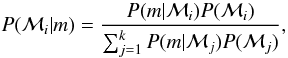$\mathit{P}\mathrm{\left(}{\mathrm{ℳ}}_{\mathit{i}}\mathrm{\right|}\mathit{m}\mathrm{)}\mathrm{=}\frac{\mathit{P}\mathrm{\left(}\mathit{m}\mathrm{\right|}{\mathrm{ℳ}}_{\mathit{i}}\mathrm{\left)}\mathit{P}\mathrm{\right(}{\mathrm{ℳ}}_{\mathit{i}}\mathrm{)}}{{\sum }_{\mathit{j}\mathrm{=}\mathrm{1}}^{\mathit{k}}\mathit{P}\mathrm{\left(}\mathit{m}\mathrm{\right|}{\mathrm{ℳ}}_{\mathit{j}}\mathrm{\left)}\mathit{P}\mathrm{\right(}{\mathrm{ℳ}}_{\mathit{j}}\mathrm{)}}\mathit{,}$(1)where P(ℳ_i) are the prior probabilities of the different models and the marginal integrals, which are sometimes called the marginal likelihoods, are defined as 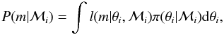$\mathit{P}\mathrm{\left(}\mathit{m}\mathrm{\right|}{\mathrm{ℳ}}_{\mathit{i}}\mathrm{)}\mathrm{=}\mathrm{\int }\mathit{l}\mathrm{(}\mathit{m}\mathrm{\left|}{\mathit{\theta }}_{\mathit{i}}\mathit{,}{\mathrm{ℳ}}_{\mathit{i}}\mathrm{\right)}\mathit{\pi }\mathrm{\left(}{\mathit{\theta }}_{\mathit{i}}\mathrm{\right|}{\mathrm{ℳ}}_{\mathit{i}}\mathrm{)}\mathrm{d}{\mathit{\theta }}_{\mathit{i}}\mathit{,}$(2)where l denotes the likelihood function and π(θ | ℳ_i) is the prior density of the parameters.

The truncated posterior-mixture estimate that approximates the marginal integral is defined as (see Appendix) $\begin{array}{ccc}\mathit{P̂}\mathrm{TPM}& \mathrm{=}& [\sum _{\mathit{i}\mathrm{=}\mathrm{1}}^{\mathit{N}}\frac{{\mathit{l}}_{\mathit{i}}{\mathit{p}}_{\mathit{i}}}{\mathrm{(}\mathrm{1}\mathrm{-}\mathit{\lambda }\mathrm{)}{\mathit{l}}_{\mathit{i}}{\mathit{p}}_{\mathit{i}}\mathrm{+}\mathit{\lambda }{\mathit{l}}_{\mathit{i}\mathrm{-}\mathit{h}}{\mathit{p}}_{\mathit{i}\mathrm{-}\mathit{h}}}]\\ & & \mathrm{\times }[\sum _{\mathit{i}\mathrm{=}\mathrm{1}}^{\mathit{N}}\frac{{\mathit{p}}_{\mathit{i}}}{\mathrm{(}\mathrm{1}\mathrm{-}\mathit{\lambda }\mathrm{)}{\mathit{l}}_{\mathit{i}}{\mathit{p}}_{\mathit{i}}\mathrm{+}\mathit{\lambda }{\mathit{l}}_{\mathit{i}\mathrm{-}\mathit{h}}{\mathit{p}}_{\mathit{i}\mathrm{-}\mathit{h}}}{]}^{-1}\mathit{,}\end{array}$(3)where l_i is the value of the likelihood function at θ_i, p_i is the value of the prior density at θ_i, and λ ∈  [0,1]  and h ∈ N are parameters that control the convergence and accuracy properties of the estimate. While it is easy to select h – it only needs to be large enough for θ_i and θ_i − h to be independent – selecting parameter λ is more difficult. If λ is too large, the sample from the posterior is not close to the sample drawn from the importance sampling function g in the Eq. (A.6) in the Appendix, and the resulting estimate of the marginal is biased. Conversely, too small values of λ, while making the estimate more accurate, decrease its convergence rate because the estimate asymptotically approaches the HM estimate that is known to have extremely poor convergence properties (see the Appendix and Kass & Raftery 1995). Therefore, we test different values of λ to find the best choice in applications. We note, however, that when θ_i and θ_i − h are independent, i.e. when h is large enough given the mixing properties of the Markov chain used to draw a sample from the posterior density, the TPM can converge to the marginal integral. The reason is that, as is clear from Eq. (3), occasional very small values of l_i, which consequently have a large impact on the sums in the estimate, do not decelerate the convergence as much as they would in the HM estimate because it is unlikely that l_i − h is also small at the same time. This is the key feature of the TPM estimate that ensures its relatively rapid convergence.

We estimate the integral in Eq. (2) using five methods. The HM estimate (see Appendix), the truncated posterior-mixture estimate introduced here, the DIC, AIC, and the OBMH method of Chib & Jeliazkov (2001). While the DIC is a reasonably practical estimate in certain cases, it requires that the posterior is unimodal and symmetric and can be approximated as a multivariate Gaussian density, which is only rarely the case in applications. It can be easily calculated by using both the average of the likelihoods and the likelihood of the parameter mean, which also reveals why the posterior needs to be unimodal and symmetric to obtain reliable results. These mean values do not reflect the properties of the posterior in cases of skewness and multiple modes, not to mention nonlinear correlations between some parameters in vector θ. The DIC is asymptotically accurate when the sample size becomes large (Spiegelhalter et al. 2002). We do not consider the HM estimate to be a trustworthy one but calculate its value because it is a special case of the truncated posterior-mixture estimate when λ = 0 (or 1). The AIC could provide a reasonably accurate estimate in practice, and therefore we compare its performance in various scenarios. However, it relies on the maximum-likelihood parameter estimate, and therefore does not take into account the prior information about the model parameters. Its accuracy also decreases as either the amount of parameters in the model increases or the number of measurements decreases. Finally, we calculate the OBMH estimate (Chib & Jeliazkov 2001). While this estimate appears to provide reliable results, e.g. the number of companions orbiting Gliese 581 determined in Tuomi (2011) was supported by additional data (Forveille et al. 2011), its performance has not been throughly studied with examples. It is also computationally more expensive than the TPM estimate, and indeed the other estimates compared here, because it requires the simultaneous sampling from the proposal density of the M-H algorithm.

When assessing the convergence of our TPM estimate given some selection of λ, we say that it has converged if the estimate at the ith member of the Markov chain, namely , satisfies for all k > 0 and some small number r, in accordance with the standard definition of convergence. However, in practice, we use the logarithms of and a value of r = 0.1 on the logarithmic scale for simplicity. For practical reasons, we also approximate the estimate as having converged if the convergence condition holds for 0 < k < 10⁵. While all the estimates except the AIC (which is based only on the maximum likelihood value) are more likely to converge the larger sample they are based on, we only plot this convergence for the TPM estimate. For DIC, HM, and OBMH, we calculate the final estimate using the mean and standard deviation of values from several samplings.

3. Prior effects on marginal integrals

Because the marginal integrals in Eq. (2) are integrals over the product of the likelihood function and the prior probability density of the model parameters, the choice of prior has an effect on these integrals for different models. One such choice for the standard model of radial velocity data was proposed in Ford & Gregory (2007) and applied in e.g. Feroz et al. (2011) and Gregory (2011). In particular, this prior limits the parameter space of jitter amplitude σ_j to [0, K₀], that of reference velocity γ to [–K₀, K₀], and that of the velocity amplitude of the ith planet, K_i, to [0, K₀(P_min/P_i)^1/3], where P_min is the shortest allowed periodicity and P_i is the orbital period of the ith planet. Ford & Gregory (2007) propose that the hyperparameter K₀ should be set to 2129 ms^-1, which corresponds to a maximum planet-star mass-ratio of 0.01.

We assume for simplicity that P_min = P_i, which leads to a constant prior for the parameter K_i. It then follows that the prior probability density of a k-Keplerian model has a multiplicative constant coefficient proportional to ${\mathit{K}}_{\mathrm{0}}^{\mathrm{-}\mathrm{2}\mathrm{-}\mathit{k}}$, which corresponds to the hypervolume of the parameter space of the k-Keplerian model. Because this constant also scales the marginal integral in Eq. (2), it can be seen that increasing K₀ can make the posterior probability of any planetary signal insufficient to claim a detection, because the ratio P(m | ℳ_k)/P(m | ℳ_k − 1) is proportional to ${\mathit{K}}_{\mathrm{0}}^{-1}$.

The above can also be described in more general terms. As indeed noted by Bartlett (1957) and Jeffreys (1961), choosing a prior for any model with parameter θ such that π(θ) = ch(θ) for all θ ∈ Θ, where Θ is the corresponding parameter space, can lead to undesired features in the model comparison results. Assume that this choice is made for model ℳ₁, but for a simpler model ℳ₀, for which parameter θ does not exist (the “null hypothesis”), this prior does not exist either because the corresponding parameter is not a free parameter of the model. The posterior probability of model ℳ₁ then becomes $\begin{array}{ccc}& & \mathit{P}\mathrm{\left(}{\mathrm{ℳ}}_{\mathrm{1}}\mathrm{\right|}\mathit{m}\mathrm{)}\mathrm{\propto }\mathit{P}\mathrm{(}\mathit{m}\mathrm{\left|}{\mathrm{ℳ}}_{\mathrm{1}}\mathrm{\right)}\mathit{P}\mathrm{\left(}{\mathrm{ℳ}}_{\mathrm{1}}\mathrm{\right)}\mathrm{=}\mathit{cP}\mathrm{\left(}{\mathrm{ℳ}}_{\mathrm{1}}\mathrm{\right)}{\mathrm{\int }}_{\mathit{\theta }\mathrm{\in }\mathrm{\Theta }}\mathit{l}\mathrm{\left(}\mathit{m}\mathrm{\right|}\mathit{\theta ,}{\mathrm{ℳ}}_{\mathrm{1}}\mathrm{\left)}\mathit{h}\mathrm{\right(}\mathit{\theta }\mathrm{)}\mathrm{d}\mathit{\theta ,}\\ & & \mathrm{where}\mathit{c}\mathrm{=}[{\mathrm{\int }}_{\mathrm{\Theta }}\mathit{h}\mathrm{\left(}\mathit{\theta }\mathrm{\right)}\mathrm{d}\mathit{\theta }{]}^{-1}\mathit{.}\end{array}$(4)Setting the prior constant such that h(θ) = 1, yields c = V(Θ)^-1, where V(Θ) denotes the hypervolume of the parameter space, and leads to the inconvenient conclusion that as the hypervolume of the parameter space Θ increases, the posterior probability of the model ℳ₁ decreases below that of the ℳ₀, which prevents the rejection of the null hypothesis regardless of the observed data m. This is called Bartlett’s paradox (Bartlett 1957; Kass & Raftery 1995) but it mean neither that improper and/or constant priors are useless nor that they should not be used in applications.

A convenient way around this “paradox”, can be achieved by considering the definition of the parameters. Because the analysis results should depend on neither the unit system of choice, nor the selected parameterisation, i.e. whether we choose parameter θ or θ′ = f(θ), where f is an invertible (bijective) function, it is possible to choose the parameter system in a convenient way to ensure that c = 1 by transforming θ′ = f(θ) with some suitable f. For some choices of f, the constant prior of parameter θ does not correspond to a constant prior for θ′, but we do not consider this well-known effect of prior choice further here.

For instance, if we apply this to a Gaussian likelihood with a mean g(θ) (e.g. a superposition of k Keplerian signals in radial velocity data) and variance σ², it becomes a value with a mean g(f(θ)) and variance σ². This does not change the posterior density of the parameters as we can always perform the inverse transformation using f^-1, but a convenient choice of f sets c = 1 and prevents the prior probability density of the parameters from having undesirable effects on the marginal integrals. A similar transformation of σ is also possible as long as the f(σ) retains the same units as the measurements. Therefore, we are free to define the model parameters in any convenient way, using e.g. any unit system, and this, as long as we retain the same functional form in our statistical model, should not be allowed to have an effect on the results of our analyses. Specifically, when analysing radial velocity data, choosing the unit system such that ${\mathit{K}}^{\mathrm{\prime }}\mathrm{=}\mathit{K}{\mathit{K}}_{\mathrm{0}}^{-1}$ changes neither the posterior density nor the values of the likelihood function but it does make π(K′) = 1 for all K′ ∈  [0,1] , which does not provide different weights for the models with different numbers of planets. We demonstrate these effects further in Sect. 5 by analysing artificial data sets.

We note that this procedure does not interfere with the Occam’s razor that is a built-in feature of Bayesian analysis methods. It remains true that, as the number of free parameters in the statistical model increases, this model also becomes more heavily penalised. The reason is that increasing the dimension of the parameter space effectively increases the hypervolume that has a reasonably high posterior probability (but lower than the MAP estimate) given the data – this increases the amount of low likelihoods in the posterior sample and in Eq. (3), which in turn decreases the estimated marginal integral as it should in accordance with the Occamian principle of parsimony.

4. Comparison of estimates: radial velocities of HD 3651

To assess the performance of the TPM estimate for the marginal integral, we compare its performance with different selections of parameter λ in simple cases where the marginal integral can be calculated reliably using the DIC, i.e. when the model parameters receive close-Gaussian posteriors and the sample size is large. Therefore, as test cases, we choose radial velocity time-series made using several telescope-instrument combinations that have different velocity offsets and different noise levels. The simple model without any Keplerian signals provides a suitable scenario where the DIC is known to be accurate and the accuracy of our estimate can be assessed in practice.

The nearby K0 V dwarf HD 3651 has been reported to be a host to a 0.20 M_Jup exoplanet with an orbital period of 62.23  ±  0.03 days and an orbital eccentricity of 0.63  ±  0.04 (Fischer et al. 2003). The radial velocity variations of HD 3651 have been observed using the HIRES at the Keck I telescope (Fischer et al. 2003; Butler et al. 2006) and the Shane and CAT telescopes at the Lick observatory (Fischer et al. 2003; Butler et al. 2006). These datasets contain measurements at 42 and 121 epochs, respectively. The reason we chose these data is that they enable us to investigate several scenarios reliably. The planet orbiting HD 3651 is on an eccentric orbit and there is plenty of data available, which makes it possible to assess the accuracy of the TPM estimate in several scenarios by enabling a comparison to the DIC estimate, which is accurate as long as the posterior density is Gaussian. Therefore, we investigate the accuracy and convergence properties of the TPM in various scenarios: with both high and low numbers of data compared to the number of model parameters, and when the marginal likelihoods of two models are close to each other and as far apart from each other as possible given the available data.

We analyse the radial velocities of HD 3651 made using the HIRES and Lick exoplanet surveys, and calculate the marginal likelihoods of models with both zero and one Keplerian signals using the methods based on DIC, AIC, TPM, HM, and OBMH. We denote these estimates of the integral in Eq. (2) as , , , , and , respectively. We also calculate the marginal integrals for a very simple case of 0-Keplerian model and HIRES data using a sample from the prior () density and direct numerical integration ().

4.1. Case 1: HIRES data

The HIRES data with 42 epochs reveals some interesting differences between the five estimates of marginal integrals. The log-marginal integrals are plotted in Fig. 1 as a function of Markov chain length. The estimated uncertainties in the DIC and OBMH estimates represent the standard deviations of six different Markov chains. The DIC estimate can be considered a reliable one in this case, because the posterior density is very close to a multivariate Gaussian. It can be seen that the AIC is biased because of the low number of measurements (namely 42) compared to the number of parameters of the statistical model (7). In addition, the OBMH estimate gives the one-planet model a greater marginal likelihood than DIC. However, the TPM is similarly biased for λ = 0.5,0.1,10^-2, and 10^-3, but converges to the DIC estimate for λ = 10^-4,10^-5. The HM estimate is not shown in the figure because of its extremely poor convergence properties – it reaches values between –130 and –140 on the logarithmic scale of Fig. 1.

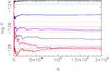Fig. 1 Marginal integrals of the one-planet model given the HIRES data (case 1): DIC and its 3σ uncertainty (black dashed line and black dotted lines), AIC (blue dashed), OBMH and its 3σ uncertainty (red dashed and red dotted), and the TPM estimates with λ = 0.5,0.1,10-2,10-3,10-4,10-5 (black, grey, blue, purple, pink, and red curves).

When using as small values of λ for the TPM as possible such that it converges in the sense that it approaches some limiting value, we calculate the Bayes factors (B) in favour of the one-Keplerian model and against the model without Keplerian signals. These values are shown in Table 1. The TPM estimate converges to the same value as DIC, which is known to be accurate in this case because the posterior densities of both models are very close to Gaussian. However, both the AIC and OBHM overestimate the posterior probability of the model containing a Keplerian signal. The problems of the HM estimate are also clear because its uncertainty becomes larger than its estimated value.

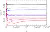Fig. 2 As in Fig. 1 but for the combined data (case 2) and the TPM estimates with λ = 0.1,10-2,10-3,10-4,10-5,10-6 (black, grey, blue, purple, pink, and red curves).

4.2. Case 2: Combined HIRES and Lick data

Increasing the number of measurements likely makes the AIC yield a more accurate estimate of the marginal likelihood. However, to see how this affects the other estimates, we again compare them to the DIC, which is reliable because of the close-to-Gaussianity of the posterior density. The inclusion of additional Lick data also makes the posterior probability of the one-Keplerian model much greater than that of the model without Keplerian signals, and enables us to investigate the accuracy and convergence of the TMP in such a scenario. Therefore, we study the properties of the different estimates for marginal integrals using the combined HIRES and Lick data of HD 3651 over 163 epochs.

The TPM estimate converges to the DIC estimate when λ = 10^-3 for the model without any Keplerians, whereas its convergence takes place for λ = 10^-5 for the one-Keplerian model (Fig. 2, pink curve). Clearly, the AIC is indeed closer to the DIC estimate because of the greater amount of data, but the OBHM is also consistent with the DIC estimate. We note that the HM estimate is again omitted from Fig. 2 because it has significantly lower values than the other estimates.

We now calculate the Bayes factors in favour of the one-Keplerian model and present them in Table 2. The TPM estimate is again very close to the DIC estimate and the AIC is close to these, providing slightly greater support for the one-Keplerian model. The OBMH again overestimates the one-Keplerian model and the HM estimate, while it is rather accurate this time, it has an uncertainty in excess of the estimate itself. The TPM estimate can clearly be used to receive reliable estimates of the marginal integral in this case as well, because the posterior density is again very close to a Gaussian one and the DIC estimate can therefore provide a reliable estimate of the integral.

4.3. Case 3: Partial HIRES data

As a third test, we calculate the different estimates of the marginal integral given only 20 epochs of HIRES data – the first 20 epochs being between 366 and 2602 JD-2450000 – to see their relative performance when the number of parameters is comparable to the number of measurements. We find that the TPM converges to the marginal integral very accurately when λ = 10^-3 for both models and yields very reliable estimates for these integrals. It is again very close to the DIC estimate, making it reliable because of the Gaussianity of the posterior density for both models and the consequent reliability of the DIC estimate. It is unsurprising that the AIC overestimates the Bayes factor and therefore also the posterior odds of the one-Keplerian model, because of the small amount of data. However, the OBMH overestimates it as well, as was also found to be the case in the test cases 1 and 2.

5. Artificial data: effect of prior choice

We now illustrate in greater detail the properties of the TPM estimate by comparing its performance to more traditional integral-estimation techniques. We generated four sets of artificial radial velocity data and determined the number of Keplerian signals using the TPM estimate and an estimate received using a brute force approach, i.e. direct numerical integration of the product of likelihood and prior over the parameter space. To demonstrate the conclusions in Sect. 3, we use an improper unit prior, i.e. π₁ = π(θ) = 1, and a broad prior of Ford & Gregory (2007) with P_min = P_i, which is denoted as π₂, to show how they affect the conclusions that can be drawn from the same data.

The artificial data sets were generated by using 200 random epochs such that the first epoch was at t = 0 and the ith one was selected randomly one to ten days later within an interval of 7.2 h, which simulates that observations can only be made during the night. We generated the velocities by using a sinusoid with a period of 50 days and an amplitude of K, and added Gaussian random noise with a zero mean and a variance of $\mathrm{1}\mathrm{+}{\mathit{\sigma }}_{\mathit{i}}^{\mathrm{2}}$, where σ_i describes the standard deviation of the artificial Gaussian instrument noise. The values σ_i were drawn from a uniform density between 0.3 and 0.6 for every simulated measurement. We generated sets S1, ..., S4 by setting K = 1.0,0.8,0.6,0.5, respectively.

We show the model comparison results of the four artificial data sets in Table 4. This table contains the Bayes factors in favour of the model with one Keplerian signal and against a model with no signals at all. We show the estimates calculated using a direct brute force numerical integration (BF) for the two priors (π₁ and π₂) and the TPM estimate, which has approximately the same values for both priors, so we show only the results for π₁. These Bayes factors show, that the Bartlett’s paradox clearly prevents the detection (i.e. a Bayes factor in excess of 150; Kass & Raftery 1995; Tuomi 2012) of the periodic signals in the data set S3, whereas the TPM estimate, which does not fall victim to this paradox, exceeds the detection threshold. The signal in the set S4 is too weak for detection.

It can be seen in Table 4 that the TPM estimate yields Bayes factors that support the existence of a signal in the data sets S1−S3. For the only data set where the signal could not be detected (S4), the Markov chains did not converge to a clear maximum in the period space either, but several small maxima, among which none could be said to be significantly more probable than the others. In all the rest, the chains converged to a clear maximum corresponding to the periodic signals added to the artificial data sets.

It can also be seen how the broader prior (π₂) changes the Bayes factors when estimating the marginal integrals by direct numerical integration. Relative to the unit prior (π₁), the Bayes factors are roughly a factor of 10⁵ lower for π₂, and actually only provide a detection of the signal in data set S2 by only slightly exceeding the 150 threshold. This shows that the π₂ corresponds to a priori model probabilities that are by a factor of 10⁵ more in favour of the model without Keplerian signals. This is clearly an undesirable side-effect of the priors of Ford & Gregory (2007). Nevertheless, the TPM estimate, and the corresponding Bayes factors, turned out to have roughly the same values for both priors as suspected, because any constant terms in the prior do not affect the TPM estimate. Therefore, the TMP estimate enables the detection of weaker signals in the data than estimates that depend on constant coefficients in the prior density and, consequently, affect the prior probabilities of the models.

6. Conclusions

Calculating the marginal integral for model selection purposes is generally a challenging computational problem. While there are several good estimates of these integrals, they are usually only applicable under certain limiting assumptions about the nature of the posterior density, the amount of parameters in the statistical model, or the number of measurements available. We have therefore introduced a new method for estimating these integrals in practice. Given the availability of a sample from the posterior density of model parameters, our truncated posterior-mixture estimate is a reasonably accurate one and very easily calculated in practice. We have only assumed that a statistically representative sample drawn from the posterior density exists when deriving our posterior mixture estimate (see Appendix). Therefore, this estimation method is applicable to any model comparison problems in astronomy and other fields of scientific inquiry, and not restricted to problems where the posterior has a certain shape and dimension.

The comparisons of different estimates given the radial velocities of HD 3651 revealed that the TPM yields estimates very close to the DIC estimate, which is known to be a reliable one in the case of a Gaussian posterior density. We chose HD 3651 as an example star because the planet orbiting it is known to have an eccentric orbit that enables us to assume Gaussianity for the probability distributions of both eccentricity and the two angular parameters of the Keplerian model, namely the longitude of pericentre and mean anomaly. However, the simple small-sample version of the AIC proved to be reasonably accurate as well when the number of measurements clearly exceeded the number of free parameters of the model (e.g. Table 2). We also note that the OBMH estimate of Chib & Jeliazkov (2001), while converging rapidly, tends to yield somewhat biased results that exaggerate the posterior probability of the more complicated model, making it possibly – at least in the test cases considered in the current work – prone to detections of false positives.

In practice, the TMP can be used by calculating its value directly from the sample drawn from the posterior density of the model parameters. Selecting a suitable value for parameter λ is then of essence when calculating its value in practice. In all the three different test cases studied in this article, a choice of λ = 10^-4 yielded estimates that converged rapidly for all the models in all the test cases, and resulted in posterior probabilities that differed little from those calculated using the DIC estimate. When the difference between the two models was at its smallest (case 3.), there was practically no bias in the TMP estimate with respect to the DIC. In addition, when the posterior odds of the one-Keplerian model were at their greatest (case 2.), the TPM, with λ = 10^-4, overestimated the posterior probability of the one-Keplerian model by a factor of ten, though, in this case, the Bayes factor used in the model selection was already so heavily in favour of the one-Keplerian model that this overestimation was not significant in practice in terms of being able to select the best model.

Because of the possible biases caused by too large a value of λ, it would then be convenient in practice to calculate the TPM estimate using a few different values of parameter λ. With the sample from the posterior density available, this could be done with little computational cost. It would then be possible to use the smallest value of λ that still converges to provide a trustworthy TPM estimate and correspondingly trustworthy model selection results in any model selection problem.

Finally, because any constant coefficients in the prior probability densities have an effect on the marginal integrals by corresponding to different prior weights for different models, we have shown how the TPM estimate deals with this problem. Effectively, using this estimate corresponds to setting the constant coefficients in the prior equal to unity, which makes the TPM estimate independent of the unit choice of the parameters.

Acknowledgments

M. Tuomi is supported by RoPACS (Rocky Planets Around Cool Stars), a Marie Curie Initial Training Network funded by the European Commission’s Seventh Framework Programme. The authors would like to acknowledge P. Gregory for fruitful comments that resulted in significant improvements of the article.

References

Appendix A: Marginal integrals from importance sampling

In the context of Bayesian model selection, the marginal integral needed to assess the relative probabilities of different model is $\mathit{P}\mathrm{\left(}\mathit{m}\mathrm{\right|}\mathrm{ℳ}\mathrm{)}\mathrm{=}{\mathrm{\int }}_{\mathit{\theta }\mathrm{\in }\mathrm{\Theta }}\mathit{l}\mathrm{(}\mathit{m}\mathrm{\left|}\mathit{\theta ,}\mathrm{ℳ}\mathrm{\right)}\mathit{\pi }\mathrm{\left(}\mathit{\theta }\mathrm{\right|}\mathrm{ℳ}\mathrm{)}\mathrm{d}\mathit{\theta ,}$(A.1)where ℳ is a model with parameter vector θ constructed to model the measurements m using the likelihood function l. Function π(θ | ℳ) is the prior probability density of the model parameters. This quantity is essential in calculating the posterior probabilities of different models in Eq. (1).

Importance sampling can be used to obtain estimates of the integral in Eq. (A.1). Choosing functions g and w such that π(θ) = w(θ)g(θ) and dropping the model from the notation, the marginal integral can be written using the expectation with respect to density g as $E_{\mathit{g}}[\mathit{w}\mathrm{\left(}\mathit{\theta }\mathrm{\right)}\mathit{l}\mathrm{\left(}\mathit{m}\mathrm{\right|}\mathit{\theta }\mathrm{)}]\mathrm{=}{\mathrm{\int }}_{\mathit{\theta }\mathrm{\in }\mathrm{\Theta }}\mathit{g}\mathrm{(}\mathit{\theta }\mathrm{\left)}\mathit{w}\mathrm{\right(}\mathit{\theta }\mathrm{\left)}\mathit{l}\mathrm{\right(}\mathit{m}\mathrm{\left|}\mathit{\theta }\mathrm{\right)}\mathrm{d}\mathit{\theta }\mathrm{=}\mathit{P}\mathrm{\left(}\mathit{m}\mathrm{\right)}\mathit{,}$(A.2)where g(θ) is usually called the importance sampling function. The idea of importance sampling is then that if we draw a sample of N values from g and denote θ_i ~ g(θ) for all i = 1,...,N, we can calculate a simple estimate for the marginal integral as (e.g. Kass & Raftery 1995) $\mathit{P̂}\mathrm{=}[\sum _{\mathit{i}\mathrm{=}\mathrm{1}}^{\mathit{N}}\frac{\mathit{\pi }\mathrm{\left(}{\mathit{\theta }}_{\mathit{i}}\mathrm{\right)}\mathit{l}\mathrm{\left(}\mathit{m}\mathrm{\right|}{\mathit{\theta }}_{\mathit{i}}\mathrm{)}}{\mathit{g}\mathrm{\left(}{\mathit{\theta }}_{\mathit{i}}\mathrm{\right)}}][\sum _{\mathit{i}\mathrm{=}\mathrm{1}}^{\mathit{N}}\frac{\mathit{\pi }\mathrm{\left(}{\mathit{\theta }}_{\mathit{i}}\mathrm{\right)}}{\mathit{g}\mathrm{\left(}{\mathit{\theta }}_{\mathit{i}}\mathrm{\right)}}{]}^{-1}\mathrm{·}$(A.3)All that remains is to choose g such that it is easy to draw a sample from it and that the estimate in Eq. (A.3) converges rapidly to the marginal integral.

Some simple choices of g would be the prior density or the posterior density. In these cases, the resulting estimates would be called the mean estimate and the harmonic mean estimate, respectively (Newton & Raftery 1994; Kass & Raftery 1995). We denote these estimates as and and write $\mathit{P̂}\mathit{M}\mathrm{=}\frac{\mathrm{1}}{\mathit{N}}\sum _{\mathit{i}\mathrm{=}\mathrm{1}}^{\mathit{N}}\mathit{l}\mathrm{\left(}\mathit{m}\mathrm{\right|}{\mathit{\theta }}_{\mathit{i}}\mathrm{)}$(A.4)and $\mathit{P̂}\mathit{HM}\mathrm{=}\mathit{N}[\sum _{\mathit{i}\mathrm{=}\mathrm{1}}^{\mathit{N}}\frac{\mathrm{1}}{\mathit{l}\mathrm{\left(}\mathit{m}\mathrm{\right|}{\mathit{\theta }}_{\mathit{i}}\mathrm{)}}{]}^{-1}\mathrm{·}$(A.5)Though easily computed in practice, these estimates have some undesirable properties. For instance, the mean estimate requires the drawing of a sample from the prior density and computation of the corresponding likelihoods. However, because the prior contains less information and is therefore a much broader density than the posterior, most of the values in this sample correspond to very low likelihoods and the convergence of this estimate is generally slow. The resulting value is also dominated by few high likelihoods, which can make it too biased to be useful in applications, except in very simple cases.

In addition, the harmonic mean estimate converges to the desired value extremely slowly in practice (Kass & Raftery 1995) and its usage cannot be recommended. In applications, this estimate does not generally converge to the marginal integral within the limited sample available from the posterior. The reason is that the occasional small values of l(m | θ_i) have a large impact on the sum, making its convergence extremely slow. For these reasons, more reliable estimates of marginal integrals are needed in model selection problems.

A.1. The posterior mixture estimate

To construct a better estimate of the marginal integral, we start by assuming that a statistically representative sample has been drawn from the posterior density using some posterior sampling algorithm. We therefore have a collection of N vectors θ_i ~ π(θ | m), for all i = 1,...,N. These values form a Markovian chain with N members. Selecting integer h > 0, the value of the posterior π(θ_i − h | m) is available if the value corresponding to θ_i is available given i > h > 0. Here we can denote π_i = π(θ_i | m) and see that if θ_i is a random vector, then π_i is some random number corresponding to the value of the posterior at θ_i. Using the notation similarly for g_i, and setting λ ∈  [0,1] , we can set ${\mathit{g}}_{\mathit{i}}\mathrm{=}\mathrm{(}\mathrm{1}\mathrm{-}\mathit{\lambda }\mathrm{)}{\mathit{\pi }}_{\mathit{i}}\mathrm{+}\mathit{\lambda }{\mathit{\pi }}_{\mathit{i}\mathrm{-}\mathit{h}}\mathit{.}$(A.6)If λ is a small number, it now follows that g_i ≈ π_i – the importance sampling function g is close to the posterior but not exactly equal. We call it a truncated posterior-mixture (TPM) function. The sample from the posterior is close to a sample from g, which is a desired property because a sample from the posterior can be calculated rather readily with posterior sampling algorithms (e.g. Metropolis et al. 1953; Hastings 1970; Haario et al. 2001). The estimate in Eq. (A.3) can now be calculated. We denote l_i = l(m | θ_i) and p_i = π(θ_i) and write the resulting posterior mixture estimate as $\begin{array}{ccc}\mathit{P̂}\mathrm{TPM}& \mathrm{=}& [\sum _{\mathit{i}\mathrm{=}\mathrm{1}}^{\mathit{N}}\frac{{\mathit{l}}_{\mathit{i}}{\mathit{p}}_{\mathit{i}}}{\mathrm{(}\mathrm{1}\mathrm{-}\mathit{\lambda }\mathrm{)}{\mathit{l}}_{\mathit{i}}{\mathit{p}}_{\mathit{i}}\mathrm{+}\mathit{\lambda }{\mathit{l}}_{\mathit{i}\mathrm{-}\mathit{h}}{\mathit{p}}_{\mathit{i}\mathrm{-}\mathit{h}}}]\\ & & \mathrm{\times }[\sum _{\mathit{i}\mathrm{=}\mathrm{1}}^{\mathit{N}}\frac{{\mathit{p}}_{\mathit{i}}}{\mathrm{(}\mathrm{1}\mathrm{-}\mathit{\lambda }\mathrm{)}{\mathit{l}}_{\mathit{i}}{\mathit{p}}_{\mathit{i}}\mathrm{+}\mathit{\lambda }{\mathit{l}}_{\mathit{i}\mathrm{-}\mathit{h}}{\mathit{p}}_{\mathit{i}\mathrm{-}\mathit{h}}}{]}^{-1}\mathrm{·}\end{array}$(A.7)

If the Markov chain has good mixing properties such that the value θ_i has already become independent of θ_i − h, the likelihoods of these values are also independent. When comparing this estimate with in Eq. (A.5), it can be seen that occasional small values of l_i do not have such a large effect on the sum in the denominator, because it is unlikely that the corresponding value of l_i − h is also small at the same time.

All Tables

All Figures

	Fig. 1 Marginal integrals of the one-planet model given the HIRES data (case 1): DIC and its 3σ uncertainty (black dashed line and black dotted lines), AIC (blue dashed), OBMH and its 3σ uncertainty (red dashed and red dotted), and the TPM estimates with λ = 0.5,0.1,10-2,10-3,10-4,10-5 (black, grey, blue, purple, pink, and red curves).
In the text

	Fig. 2 As in Fig. 1 but for the combined data (case 2) and the TPM estimates with λ = 0.1,10-2,10-3,10-4,10-5,10-6 (black, grey, blue, purple, pink, and red curves).
In the text

References

- Akaike, H. 1973, in Second International Symposium on Information Theory, Akadémiai Kiadó, eds. B. N. Petrov, & F. Csaki, 1, 267 [Google Scholar]
- Barge, P., Baglin, A., Auvergne, M., et al. 2007, A&A, 482, L17 [Google Scholar]
- Bartlett, M. S. 1957, Biometrika, 44, 533 [Google Scholar]
- Bean, J. L., Seifahrt, A., Hartman, H., et al. 2010, ApJ, 711, L19 [NASA ADS] [CrossRef] [Google Scholar]
- Benedict, G. F., McArthur, B. E., Forveille, T., et al. 2002, ApJ, 581, L115 [NASA ADS] [CrossRef] [Google Scholar]
- Burnham, K. P., & Anderson, D. R. 2002, Model selection and multimodel inference: A practical information-theoretic approach (Springer-Verlag) [Google Scholar]
- Butler, R. P., Wright, J. T., Marcy, G. W., et al. 2006, ApJ, 646, 505 [NASA ADS] [CrossRef] [Google Scholar]
- Chib, S., & Jeliazkov, I. 2001, J. Am. Stat. Ass., 96, 270 [Google Scholar]
- Clyde, M. A., Berger, J. O., Bullard, F., et al. 2007, Statistical Challenges in Modern Astronomy IV, eds. G. J. Babu, & E. D. Feigelson, ASP Conf. Ser., 371, 224 [Google Scholar]
- Collier Cameron, A., Bouchy, F., Hébrard, G., et al. 2007, MNRAS, 375, 951 [NASA ADS] [CrossRef] [Google Scholar]
- Faedi, F., Barros, S. C. C., Anderson, D. R., et al. 2011, A&A, 531, A40 [NASA ADS] [CrossRef] [EDP Sciences] [Google Scholar]
- Feroz, F., Balan, S. T., & Hobson, M. P. 2011, MNRAS, 415, 3462 [NASA ADS] [CrossRef] [Google Scholar]
- Fischer, D. A., Butler, R. P., Marcy, G. W., et al. 2003, ApJ, 590, 1081 [NASA ADS] [CrossRef] [Google Scholar]
- Ford, E. B., & Gregory, P. C. 2007, Statistical Challenges in Modern Astronomy IV, eds. G. J. Babu, & E. D. Feigelson, ASP Conf. Ser., 371, 189 [Google Scholar]
- Forveille, T., Bonfils, X., Delfosse, X., et al. 2011, A&A, submitted [arXiv:1109.2505] [Google Scholar]
- Gregory, P. C. 2005, ApJ, 631, 1198 [NASA ADS] [CrossRef] [Google Scholar]
- Gregory, P. C. 2007a, MNRAS, 381, 1607 [NASA ADS] [CrossRef] [MathSciNet] [Google Scholar]
- Gregory, P. C. 2007b, MNRAS, 374, 1321 [NASA ADS] [CrossRef] [Google Scholar]
- Gregory, P. C. 2011, MNRAS, 415, 2523 [NASA ADS] [CrossRef] [Google Scholar]
- Haario, H., Saksman, E., & Tamminen, J. 2001, Bernoulli, 7, 223 [CrossRef] [MathSciNet] [Google Scholar]
- Hastings, W. 1970, Biometrika 57, 97 [Google Scholar]
- Hébrard, G., Evans, T. M., Alonso, R., et al. 2011. A&A, 533, A130 [Google Scholar]
- Holman, M. J., & Murray, N. W. 2005, Science, 307, 1288 [NASA ADS] [CrossRef] [PubMed] [Google Scholar]
- Jeffreys, H. 1961, Theory of Probability, Oxford University Press [Google Scholar]
- Jones, H. R. A., Butler, R. P., Marcy, G. W., et al. 2002, MNRAS, 337, 1170 [NASA ADS] [CrossRef] [Google Scholar]
- Kass, R. E., & Raftery, A. E. 1995, J. Am. Stat. Ass., 430, 773 [Google Scholar]
- Kullback, S., & Leibler, R. A. 1951, Ann. Math. Stat., 22, 76 [Google Scholar]
- Lovis, C., Ségransan, D., Mayor, M., et al. 2011, A&A, 528, A112 [NASA ADS] [CrossRef] [EDP Sciences] [Google Scholar]
- Mayor, M., Pepe, F., Queloz, D., et al. 2003, Messenger, 114, 20 [Google Scholar]
- Metropolis, N., Rosenbluth, A. W., Rosenbluth, M. N., et al. 1953, J. Chem. Phys., 21, 1087 [NASA ADS] [CrossRef] [Google Scholar]
- Newton, M. A., & Raftery, A. E. 1994, J. Roy. Stat. Soc. B, 56, 3 [Google Scholar]
- Pravdo, S. H., & Shaklan, S. B. 2009, ApJ, 700, 623 [NASA ADS] [CrossRef] [Google Scholar]
- Spiegelhalter, D. J., Best, N. G., Carlin, B. P., & van der Linde, A. 2002, JRSS B, 64, 583 [Google Scholar]
- Tinney, C. G., Butler, R. P., Marcy, G. W., et al. 2001, ApJ, 551, 507 [NASA ADS] [CrossRef] [Google Scholar]
- Tuomi, M. 2011, A&A, 528, L5 [NASA ADS] [CrossRef] [EDP Sciences] [Google Scholar]
- Tuomi, M. 2012, A&A, 543, A52 [NASA ADS] [CrossRef] [EDP Sciences] [Google Scholar]
- Tuomi, M., & Kotiranta, S. 2009, A&A, 496, L13 [NASA ADS] [CrossRef] [EDP Sciences] [Google Scholar]
- Tuomi, M., Pinfield, D., & Jones, H. R. A. 2011, A&A, 532, A116 [NASA ADS] [CrossRef] [EDP Sciences] [Google Scholar]
- Vogt, S. S., Allen, S. L., Bigelow, B. C., et al. 1994, SPIE Instrumentation in Astronomy VIII, eds. D. L. Crawford, E. R. Craine, 2198, 362 [Google Scholar]
- Vogt, S. S., Butler, R. P., Rivera, E. J., et al. 2010, ApJ, 723, 954 [NASA ADS] [CrossRef] [EDP Sciences] [Google Scholar]