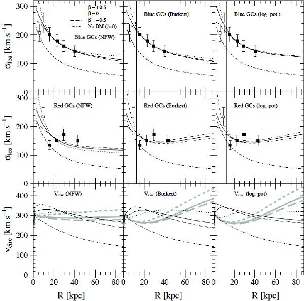
Observed and modelled GC velocity dispersion profiles. Top row: models for the blue GCs (sample BlueFinal). From left to right, the panels show the best-fit models for an NFW halo, Burkert halo and the logarithmic potential. The solid lines are the isotropic models, dashed and short-dashed lines are the tangential (β =  −0.5) and radial (β =  + 0.5) models, respectively. The dash-dotted line is the (isotropic) model without dark matter. The thin vertical line at  ≃ 13 kpc indicates the radial range inside which blue and red GCs cannot be distinguished. The data points used in the modelling are shown as filled squares (see also Table 7). The model parameters are listed in Table 9. Middle row: the same for the red GCs (RedFinal). Bottom row: circular velocity curves for the best-fit models. Again, from left to right, the results for the NFW halo, Burkert halo and the logarithmic potential are shown. The line styles are the same as in the upper graphs, with thin black lines for the blue GCs while the respective models for the red GCs are shown as thick grey lines.