| Issue |
A&A
Volume 543, July 2012
|
|
|---|---|---|
| Article Number | L6 | |
| Number of page(s) | 4 | |
| Section | Letters | |
| DOI | https://doi.org/10.1051/0004-6361/201219487 | |
| Published online | 03 July 2012 | |
Anomaly distribution of quasar magnitudes: a test of lensing by a hypothetic supergiant molecular cloud in the Galactic halo
Laboratoire Univers et Particules, UMR5299 CNRS-In2p3/Montpellier
University,
34095
Montpellier,
France
Laboratoire d’Astrophysique de Marseille,
UMR7236 CNRS-INSU/Aix-Marseille University,
13388
Marseille,
France
e-mail: This email address is being protected from spambots. You need JavaScript enabled to view it.
Received: 26 April 2012
Accepted: 12 June 2012
Abstract
Context. An anomaly in the distribution of quasar magnitudes based on the Sloan Digital Sky survey, was reported by Longo. The angular size of this quasar anomaly is on the order of ±15° on the sky. A smooth low surface brightness structure detected in γ-rays and at 408 MHz, coincides with the sky location and extent of the anomaly, and is close to the northern component of a pair of γ-ray bubbles discovered in the Fermi Gamma-ray Space Telescope survey. Molecular clouds are thought to be illuminated by cosmic rays. Molecular gas in the Galaxy, in the form of cold H2, may be a significant component of dark matter as suggested by Pfenniger et al.
Aims. I test the hypothesis that the magnitude anomaly in the quasar distribution, is due to lensing by a hypothetical supergiant molecular cloud (SGMC) either in or falling into the Galactic halo.
Methods. A series of grid lens models are built by assuming that a SGMC is a fractal structure constructed with clumps of 10-3 M⊙, 10 AU in size, and considering various fractal dimensions. Local amplifications are computed by using the single-plane approximation.
Results. A complex network of caustics due to the clumpy structure is present. Our best single plane lens model capable of explaining Longo’s effect, at least in sparse regions, requires a mass (1.5−4.1) × 1010 M⊙ within 8.7 × 8.7 × (5−8.6) kpc3 at a lens plane distance of 20 kpc, and is constructed from a molecular-cloud building-block of 5 × 10⁵ M⊙ within a scale of 30 pc expanded by fractal scaling with dimension D = 1.8−2 out to 5−8.6 kpc for the SGMC. The mass budget depends on the cloud depth and on the fractal dimension.
Conclusions. If such a SGMC were found to exist, it may provide at least part of a lensing explanation for the luminous anomaly discovered in quasars and red galaxies.
Key words: gravitational lensing: micro / ISM: clouds / Galaxy: halo / quasars: general / dark matter / gamma rays: ISM
© ESO, 2012
1. Introduction
An anomaly in the distribution of quasar magnitudes based on the Sloan Digital Sky Survey (SDSS), was reported by Longo (2012). The effect, which is an enhancement on the order of 0.2 mag, is statistically extremely significant in amplitude, and rather well-defined in angular size. A first hint of this anomaly was visible in quasar data as early as three decades ago (Giraud & Vigier 1983). Abate & Feldman (2012) reported a similar enhancement in the distribution of SDSS luminous red galaxies. Because the luminous anomaly does not seem to depend on color, a possible physical explanation is gravitational lensing. Nevertheless, if the lens is at a cosmological distance, its huge angular extent translates into a lens radius ~350 Mpc, and its critical surface density implies a total mass on the order of 1021 M⊙, which is barely consistent with ΛCDM cosmology. A major reason to test a lensing hypothesis with a lens at a short distance from the observer, possibly in the Galactic halo, is the large angular extent of the effect combined with its low amplitude.
Main parameters for lens mass models.
Two large γ-ray low-surface-brightness bubbles, extending 50° above and below the Galactic center were discovered by Su et al. (2010) in the Fermi Gamma-ray Space Telescope survey. These bubbles are spatially correlated with a microwave excess in WMAP. Both the Fermi bubbles and the WMAP haze can be explained in terms of synchrotron and inverse-Compton radiation from a hard electron population (Dobler et al. 2010). In addition to the bubbles in the Fermi map, there is a single large faint structure east of the northern bubble (l ≈ −60°, b ≈ 60°), which coincides with the quasar anomaly. Any molecular cloud, if present in this faint structure, would be illuminated by cosmic rays escaping from the northern bubble. Cosmic ray/nucleon interactions in molecular clouds were discussed by e.g. Aharonian & Atoyan (1996), de Paolis et al. (1999), Kalberla et al. (1999), Sciama (1999), and Shchekinov (2000). The spectra of γ-rays arising from molecular clouds illuminated by cosmic rays were re-examined by Ohira et al. (2011). The angular extension of the γ-ray structure is consistent with that of the quasar luminosity anomaly. We make the working hypothesis that γ-rays coming from the faint structure trace a supergiant cold molecular cloud (SGMC) in the Galactic halo.
A large fraction of molecular gas in the Galaxy is in the form of cold H2, and may be a significant component of dark matter (Pfenniger et al. 1994). The variation in the universal rotation curves (Persic et al. 1996) with mass in spiral galaxies may be interpreted as an increasing fraction of baryonic dark matter with decreasing mass of galaxies (Giraud 2000a,b, 2001). The fractal structures of molecular gas clouds, their formation, thermodynamics, and stability have been intensively studied (Scalo 1985; Henriksen 1991; Falgarone et al. 1991; Walker & Wardle 1998; Irwin et al. 2000). The existence of small dark clumps of gas in the Galaxy has been invoked to explain extreme scattering events of quasars (Fielder et al. 1987, 1994). The duration of these events suggests that the sizes and masses of individual cloudlets are on the order of 10 AU and 10-3 M⊙. These values of mass and size are also consistent with the searches for lensing toward the LMC (Draine 1998). Cloudlets can survive if the number of collisions is sufficiently small, and their stability is best explained if they are self-gravitating (Combes 2000). Concerning lensing, the average surface density of a SGMC would be sub-critical, but the chaotic structure of the matter distribution may lead to a network of caustics with high local magnification.
In the present Letter, I test the hypothesis that the magnitude anomaly in the quasar distribution can be explained in terms of lensing by a hypothetic SGMC in the Galactic halo.
2. Micro lensing and cloud lens models
2.1. Introduction
The lensing of distant galaxies and quasars shears and magnifies their images. There are extensive reviews and books written on lensing including Schneider et al. (1992), Mellier (1999), Schneider (2005), and public algorithms. Fundamental theory, ray-tracing algorithms (Valle & White 2003), and observational techniques have been developed for two to three decades to infer cluster mass distributions (Gladders et al. 2002), large-scale structures, and cosmological models (Soucail et al. 2004; Wambsganss et al. 1997, 2004; Sand et al. 2005).
Systematic studies of micro-lensing were initiated in the early 90s, by Wambsganss (1990), who developed ray-shooting simulations to show the magnification pattern of star fields. In the present paper, we use mainly the software LensTool (Jullo et al. 2007), which includes strong and weak lens regimes.
The change in direction of a light ray can be written  where da is the bend angle, grad is the spatial gradient perpendicular to the light path, φ is the gravitational potential, and χ is the radial co-moving coordinate. The distortion can be entirely described by the linearized lens mapping through the Jacobi matrix A of transform. This matrix is normally expressed with three terms depending on the derivatives of the lensing potential: the convergence κ, the amplitude of the shear γ, and the rotation ω. The convergence changes the radius of a circular source, the shear changes its ellipticity, and the rotation angle is the phase of the shear. Rotation occurs in the case of multiple lens planes.
The convergence  at location θ is related to the projected surface density Σ(θ) at that location by κ(θ) = Σ(θ)/Σcrit in which the critical surface density Σcrit is given by
  where Ds, Dl, and Dls are, respectively, the distances from observer to source, from observer to lens, and from lens to source. The shear components are
  and γ2 = ∂1∂2 φ.
The present Letter focusses on micro-lensing by numerous clumps; the convergence and the shear of any underlying smooth component is ignored.
2.2. Preliminary test lens models
The critical surface density of a smooth lens located in the Galactic halo on distant objects such that Ds ≈ Dls and assuming Dl = 15 kpc is found to be 105 M⊙ pc-2, which leads to a mass of 1014 M⊙ for a kpc scale SGMC, hence a 3D filling factor on the order of 10-4 is required to fit in the halo. A series of grid models of a kpc-size depth, with individual clumps of mass 10-3 M⊙, 10 AU in diameter, were developed with various filling factors.
The cloud models were constructed as follows: an initial FITS frame of 4000 × 4000 pixels with zero intensity including grids on the order of 10−100 pixels with a common value of one was created, so that typical separations on the order of △ ~10 000 AU were reached by assuming a physical pixel size of 10 AU. A series of layers were obtained by randomly shifting the coordinates of the initial frame, which we co-added. We repeated this shift-and-add procedure on the first co-added layer to get a second generation, and repeated again the process up to the required number of generations.
Lens mass models were obtained by multiplying the final frames by the mass of an individual clump, assuming that luminous pixels are point masses. Lens simulations with LensTool were done for small sections of the final frames.
Main parameters for fractal lens mass models.
Three cases were first considered: κ = 0.2, to enable us to compare our simulations with those in the literature, κ = 0.09 because the theoretical mean amplification calculated from ⟨μ⟩ = 1/|(1 − κ)2 − γ2| and assuming γ = 0 is that of Longo’s effect ⟨μ⟩ = 1.2, and κ = 0.8 and 0.9 to explore cases with high magnification and dense caustics. In the case κ = 0.2, individual caustics can be identified, there are perturbations of single-point caustics by other point masses giving complicated caustic structures comparable with those shown in Wambganss (1990). For κ = 0.09, the magnification pattern differs from the case κ = 0.2: individual caustics can be identified but there is almost no perturbation of single clump caustics by other clumps presumably because the density is low. For κ = 0.8, the magnification pattern shows that there is a high clustering of caustics, with huge amplification at some locations. Model parameters are in Table 1.
Reducing the size of the grid cells quickly boosts the amplification. All these kpc3 test models however are by far too massive to be used as elementary modules of a SGMC on the order of 500 kpc3. Low filling factors are necessary.
2.3. Constrained lens models
Our lens mass-models must have densities lower than the limit of molecular cloud cores: if we assume a maximum mass ~10 M⊙ within a scale length of L ~ 0.1 pc above which molecular clouds would collapse (Kayama et al. 1996), and extrapolate this density using the Larson (1981) scaling law ρ ∝ L-1.1, one gets an upper limit density ~350 M⊙ pc-3 for a scale length of ~100 pc. While our densities satisfy this criterium, a molecular cloud in equilibrium with scale 30 pc, close to our building block, would have a typical mass ~5 × 10⁵ M⊙ (Solomon et al. 1987), and a density 18.5 M⊙ pc-3, which is significantly below that of models D, E, and F.
A solution may come from a fractal structure of molecular clouds where rather small cells satisfying the equilibrium condition, are separated by less dense regions, and assembled in giant molecular clouds up to a SGMC, as proposed by Pfenniger & Combes (1994, hereafter PC) for cold dark H2 clouds. A cloud cell of 5 × 10⁵ M⊙ for a scale 30 pc is used as a building block for fractal SGMC models below.
If masses obey a fractal scaling relation with dimension D from mass Mmin to Mmax and scale Lmin to Lmax, one may write  up to Lmax. The mass at level l consists in a number of clumps N at level l − 1 related to the scale by the relation: Ll − 1/Ll = N−1/D. Clouds can survive if the number of collisions is sufficiently small, which according to PC and Irwin et al. (2000) requires 1 ≤ D ≤ 2. If D ≥ 2.33, internal and external collisions are too numerous to maintaini a fragmented cloud. Two cloud models with two fractal dimensions are considered first: the case D = 1.64, which was suggested in the original PC paper, and the upper value of D = 2.
Extrapolating from Lmin = 30 pc, and Mmin = 5 × 10⁵ M⊙ to Lmax = 5 kpc, and assuming a fractal dimension D = 1.64, one gets a total mass Mmax = 2.2 × 10⁹ M⊙ within 125 kpc3, and N ~ 4500 cloud cells, i.e. ~16 building blocks on each axis. The surface density integrated over a column Lmax = 5 kpc of 16 blocks is Σ = 8.9 × 10³ M⊙ pc-2, which is its maximum value. Parameters of this model are given in Table 2 (model G). The median magnification derived from the probability p(n) of a light ray crossing 0 ≤ n ≤ 16 cloud blocks, is found to be ∑ μ(n)p(n) = 1.03, so half the surface provides a magnification between 1.20 and 1.03, which is insufficient to explain Longo’s effect.
The case D = 2 has different properties (model H). Being more populated than for D = 1.67, the densities are higher, the median amplification is μ = 1.12, and 25% of the surface has 1.18 ≤ μ ≤ 1.48. Regions with μ ≥ 1.18 do show networks of caustics and non-Gaussian amplification distributions. Model H appears to be at the limit of explaining Longo’s effect with a mass of 4.1 × 10¹⁰ M⊙ within 28°. Explaining Longo’s effect with greater confidence would require a larger distance and depth of the lens.
2.4. Distance to the lens plane and depth of the lens
Locating the lens plane at an observer distance Dl = 20 kpc rather than 16 kpc, reduces the critical surface density by 25% to Σcrit = 7.5 × 10⁴ M⊙ pc-2 for infinitely distant objects. For this critical surface density, the same amplifications as in model H, are obtained for a cloud with D = 1.80, a mass 5 × 10⁹ M⊙ within 125 kpc3, and a total mass 1.5 × 10¹⁰ M⊙ for a SGMC that is 5 kpc in depth and extends over 8.7 × 8.7 kpc2 (model I).
Increasing the depth to 8.6 kpc and using a dimension D = 2, we obtain model J, which provides a median amplification of μ = 1.15, with 14% of the surface being amplified by more than 1.5. The total mass within 8.6 × 8.6 × 8.6 kpc3 is 4.1 × 10¹⁰ M⊙.
A single-plane lens model was assumed. If the cloud were spread over a large distance in depth, the distant part of the lens would be more efficient than the nearby one. There would be a distance shift between the illuminated area and the average lens plane.
2.5. Shear
The shear was not considered in our models. This is because the shear is a term resulting from the mass outside the light beam, such as a smooth galactic component in a star field. In our case however, cloud blocks are mass concentrations that may induce a shear component. Shear is found to be significant in grid sections of average amplification μ = 1.1 and above, but there is a large spread. Assuming γ = κ, the amplification would slightly change, so the same amplifications as for model with D = 2 would be obtained with D = 1.93.
To summarize, the local lensing hypothesis requires a lens with linear size twice that of the LMC, and a mass a few times that of this satellite. A major difference between the SGMC and the LMC in terms of lensing, is that the SGMC is fully transparent without dust, and is populated by billions of objects with a mass similar to Jupiter.
2.6. Detectability
The SGMC coincides with a ~18−28 K region in the 408 MHz survey from Haslam et al. (1982), as shown in Fig. 1 (also visible at 1.4 GHz). The coincidence between the Fermi map and that at 408 MHz can be understood if both originate from the same cosmic-ray populations (Su et al. 2010). This may occur at the front of the SGMC or in an ISM feature in the foreground.
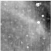 |
Fig. 1 Temperature map at 408 MHz of the field 30° × 30° centered at RA = 195°, Dec = 0°, from Haslam et al. (1982). |
Emission from CO is commonly used to trace H2. With a high column density in H2, owing to the large depth of the cloud, 3−4 × 1024 cm-2, one may expect a rather high value of integrated CO. The conversion factor XCO = NH2/WCO, however, depends strongly on the cloud optical thickness. Glover & Mac Low (2011) obtained a sharp fall-off in  with visual extinction. From the empirical relation XCO = 2 × 10²⁰ (AV/3.5)-3.5 cm-2 K-1 km-1 s, we obtain WCO < 0.1 K km s-1 for AV < 0.1.
A region of shock in front of the SGMC might produce HI. The HI column density from Dickey & Lockman (1990) in our 30° × 30° field has in fact a low value of 1.5−3 × 1020 cm-2.
2.7. Dynamical constraints and long time evolution
The internal kinematics and stability conditions of the SGMC must be similar to those of the LMC, which indicates that it is dynamically stable, despite experiencing internal velocities as high as 220 km s-1. Because the SGMC does not show evidence of HI, Hα, dust and star formation, it should be entering the Galaxy halo for the first time, while being at the location of an encounter. Owing to the findings for the LMC, a SGMC is able to cross the Galactic plane without being disrupted, although it does produce long tails. If the SGMC is falling toward the Galactic plane, it will experience tidal forces, ram pressure, UV and shock heating. Star formation may be triggered while crossing the Galactic plane, and the SGMC may become an irregular dwarf satellite.
2.8. H2 clumps and WIMPS
H2 clumps are extremely dense compared to WIMP clumps of the same mass, as predicted by N-body simulations (Diemand et al. 2005; Springel et al. 2008). A WIMP clump seeded by an H2 clump of the same mass M = 10-3 M⊙ will experience a first infall during which its density will increase by 106 in ~1 Myr. If WIMPS are low-mass neutralinos of mχ ~ 10 GeV that have an annihilation cross-section σV = 0 = 10-26 cm3 s-1 (Cerdeno et al. 2012), those concentrated in a clump will experience significant annihilation, leading to a mass transform 1.4 × 10⁻⁷ M⊙ Myr-1 mainly into p, p− and γ. The cumulated mass-loss of those neutralinos is 50% in ~6 Gyr, thus an upper limit of ~50% of the clump mass may remain in WIMPs within 10 AU over cosmological ages.
3. Conclusion
A luminosity excess of 0.2 mag was discovered in an SSDS survey of quasars. This effect, which has a huge spatial extent on the order of 30°, is extremely well-determined statistically, and coincides with a large and diffuse region detected in γ-ays by the Fermi Gamma-ray Space Telescope.
We have made the working hypothesis that the detected γ luminosity traces a SGMC illuminated by cosmic rays, at least at its front-end, and test the hypothesis of whether such a cloud would be capable of explaining the quasar luminosity excess by micro-lensing.
Cloud models are built by using compact clumps of mass 10-3 M⊙, 10 AU in size, as implied by extreme scattering events on quasars, typical molecular cloud building blocks of mass 5 × 10⁵ M⊙ for a scale of 30 pc, and a fractal structure of the SGMC with dimension 1.64 ≤ D ≤ 2 up to a scale of 5−8.6 kpc.
A SGMC located at a distance of Dl = 20 kpc from the observer, that is 8.6 kpc in depth and has a fractal dimension D = 2 appears to be capable of explaining Longo’s effect with a mass of 4.1 × 10¹⁰ M⊙, which is four times that of the LMC.
Acknowledgments
This paper is dedicated to the memory of Jean-Pierre Vigier. I thank L. Falletti, N. Mauron, M. Renaud, J. Lavalle, and the referee.
References
- Abate, A., & Feldman, H. 2012, MNRAS, 419, 3482 [NASA ADS] [CrossRef] [Google Scholar]
- Aharonian, F. A., & Atoyan, A. 1996, A&A, 309, 917 [NASA ADS] [Google Scholar]
- Cerdeno, D. G., Delahaye, T., & Lavalle, J. 2012, Nucl. Phys. B, 854, 738 [NASA ADS] [CrossRef] [Google Scholar]
- Combes, F. 2001, in Molecular hydrogen in space, eds. F. Combes, & G. Pineau des Forłts (Cambridge University Press), 275 [Google Scholar]
- de Paolis, F., Ingrosso, G., Jetzer, P., & Roncadelli, M. 1999, ApJ, 510, L103 [NASA ADS] [CrossRef] [Google Scholar]
- Dickey, J. M., & Lockam, F. J. 1990, ARA&A, 28, 215 [NASA ADS] [CrossRef] [MathSciNet] [Google Scholar]
- Diemand, J., Moore, B., & Stadel, J. 2005, Nature, 433, 389 [NASA ADS] [CrossRef] [Google Scholar]
- Dobler, G., Finkbeiner, D. P., Cholis, I., Slatyer, T. R., & Weiner, N. 2010, ApJ, 717, 825 [NASA ADS] [CrossRef] [Google Scholar]
- Draine, B. T. 1998, ApJ, 509, 41 [Google Scholar]
- Falgarone, E., Phillips, T. G., & Walker, C. K. 1991, ApJ, 378, 186 [NASA ADS] [CrossRef] [Google Scholar]
- Fiedler, R. L., Dennison, B., Johnston, K. J., & Hewish, A. 1987, Nature, 326, 675 [NASA ADS] [CrossRef] [Google Scholar]
- Fiedler, R., Dennison, B., Johnston, K. J., Waltman, E. B., & Simon, R. S. 1994, ApJ, 430, 581 [NASA ADS] [CrossRef] [Google Scholar]
- Giraud, E. 2000a, ApJ, 544, L41 [NASA ADS] [CrossRef] [Google Scholar]
- Giraud, E. 2000b, ApJ, 539, 115 [NASA ADS] [CrossRef] [Google Scholar]
- Giraud, E. 2001, ApJ, 558, L23 [NASA ADS] [CrossRef] [Google Scholar]
- Giraud, E., & Vigier, J.-P. 1983, in Quasars and Gravitational Lenses, Liège International Astrophysical Colloquium LIACo, 24, 380 [Google Scholar]
- Gladders, M. D., Yee, H. K. C., & Ellingson, E. 2002, AJ, 123, 1 [NASA ADS] [CrossRef] [Google Scholar]
- Glover, S. C. O., & Mac Low, M.-M. 2011, MNRAS, 412, 337 [NASA ADS] [CrossRef] [MathSciNet] [Google Scholar]
- Haslam, C. G. T., Salter, C. J., Stoffel, H., & Wilson, W. E. 1982, A&AS, 47, 1 [NASA ADS] [Google Scholar]
- Henriksen, R. N. 1991, ApJ, 377, 500 [NASA ADS] [CrossRef] [Google Scholar]
- Irwin, J. A., Widraw, L. M., & English, J. 2000, ApJ, 529, 77 [NASA ADS] [CrossRef] [Google Scholar]
- Jullo, E., Kneib, J.-P., Limousin, M., et al. 2007, New J. Phys., 9, 447 [Google Scholar]
- Kalberla, P. M. W., Shchekinov, Y. A., & Dettmar, R.-J. 1999, A&A, 350, L9 [NASA ADS] [Google Scholar]
- Kamaya, H. 1996, ApJ, 466, L99 [NASA ADS] [CrossRef] [Google Scholar]
- Longo, M. J. 2012 [arXiv:1202.4433] [Google Scholar]
- Mellier, Y. 1999, ARA&A, 37, 127 [NASA ADS] [CrossRef] [Google Scholar]
- Ohira, Y., Murase, K., & Yamazaki, R. 2011, MNRAS, 410, 1577 [NASA ADS] [Google Scholar]
- Persic, M., Salucci, P., & Stel, F. 1996, MNRAS, 281, 27 [NASA ADS] [CrossRef] [Google Scholar]
- Pfenniger, D., & Combes, F. 1994, A&A, 285, 94 [NASA ADS] [Google Scholar]
- Pfenniger, D., Combes, F., & Martinet, L. 1994, A&A, 285, 79 [NASA ADS] [Google Scholar]
- Sand, D. J., Treu, T., Ellis, R. S., & Smith, G. P. 2005, ApJ, 627, 32 [NASA ADS] [CrossRef] [Google Scholar]
- Sciama, D. W. 2000a, MNRAS, 319, 1001 [NASA ADS] [CrossRef] [Google Scholar]
- Sciama, D. W. 2000b, MNRAS, 312, 33 [NASA ADS] [CrossRef] [Google Scholar]
- Scalo, J. M. 1985, in Protostars & Planets II, eds. D. C. Black, & M. S. Matthews (Tucson: Univ. Arizona Press), 201 [Google Scholar]
- Schneider, P. 2005, in Gravitational Lensing: Strong, Weak & Micro, eds. G. Meylan, P. Jetzer, & P. North (Berlin: Springer-Verlag), 273 [Google Scholar]
- Schneider, P., Ehlers, J., & Falco 1992, Gravitational Lenses (Berlin: Springer-Verlag) [Google Scholar]
- Shchekinov, Y. 2000, Astron. Rep., 44, 65 [NASA ADS] [CrossRef] [Google Scholar]
- Solomon, P. M., Rivolo, A. R., Barrett, J., & Yahil, A. 1987, ApJ, 319, 730 [NASA ADS] [CrossRef] [Google Scholar]
- Springel, V., White, S. D. M., Frenk, C. S., et al. 2008, Nature, 456, 73 [NASA ADS] [CrossRef] [PubMed] [Google Scholar]
- Soucail, G., Kneib, J.-P., & Golse, G. 2004, A&A, 417, L33 [NASA ADS] [CrossRef] [EDP Sciences] [Google Scholar]
- Su, M., Slatyer, T. R., & Finkbeiner, D. P. 2010, ApJ, 724, 1044 [NASA ADS] [CrossRef] [Google Scholar]
- Vale, C., & White, M. 2003, ApJ, 592, 69 [NASA ADS] [Google Scholar]
- Walker, M., & Wardle, M. 1998, ApJ, 498, L125 [NASA ADS] [CrossRef] [Google Scholar]
- Wambsganss, J. 1990, Gravitational Microlensing, Max Planck report 550, MPA Garching [Google Scholar]
- Wambsganss, J., Cen, R., Xu, G., & Ostriker, J. P. 1997, ApJ, 475, L81 [NASA ADS] [CrossRef] [Google Scholar]
- Wambsganss, J., Bode, P., & Ostriker, J. P. 2004, ApJ, 606, L93 [NASA ADS] [CrossRef] [Google Scholar]
All Tables
All Figures
|
Fig. 1 Temperature map at 408 MHz of the field 30° × 30° centered at RA = 195°, Dec = 0°, from Haslam et al. (1982). |
| In the text | |
Current usage metrics show cumulative count of Article Views (full-text article views including HTML views, PDF and ePub downloads, according to the available data) and Abstracts Views on Vision4Press platform.
Data correspond to usage on the plateform after 2015. The current usage metrics is available 48-96 hours after online publication and is updated daily on week days.
Initial download of the metrics may take a while.