| Issue |
A&A
Volume 543, July 2012
|
|
|---|---|---|
| Article Number | A91 | |
| Number of page(s) | 7 | |
| Section | Cosmology (including clusters of galaxies) | |
| DOI | https://doi.org/10.1051/0004-6361/201219348 | |
| Published online | 03 July 2012 | |
Current constraints on early dark energy and growth index using latest observations
1 School of Astronomy and Space Science, Nanjing University, 210093 Nanjing, PR China
e-mail: This email address is being protected from spambots. You need JavaScript enabled to view it.
2 Key laboratory of Modern Astronomy and Astrophysics (Nanjing University), Ministry of Education, 210093 Nanjing, PR China
Received: 5 April 2012
Accepted: 18 May 2012
Abstract
Aims. In this paper we study observational constraints on early dark energy model proposed by Doran & Robbers and growth index using the latest Union2 type Ia supernovae (SNe Ia), the baryon acoustic oscillations (BAO) in the large-scale correlation function of the Sloan Digital Sky Survey and Two-degree Field Galaxy Redshift Survey, cosmic microwave background (CMB) from the Wilkinson Microwave Anisotropy Probe seven-year data, the linear growth factors data and gamma-ray bursts (GRBs).
Methods. By using the χ2 statics method, we constrain the early dark energy model and growth factor from the above datasets. When including the GRB data, we use the cosmographic parameters to calibrate the GRB luminosity relations using SNe Ia.
Results. At 2σ confidence level, we find that the fractional dark energy density at early times is Ωde<0.05 using SNe Ia, CMB and BAO. When we include high-redshift probes, such as measurements of the linear growth factors and GRBs, the constraint is tightened considerably and becomes Ωde<0.03 at 2σ confidence level. We also discuss the growth rate index γ. We find γ = 0.661-0.203+0.302(1σ) using the SNe Ia, CMB, BAO and linear growth factor data. After including high-redshift GRB data, the growth index is γ = 0.653-0.363+0.372.
Key words: dark energy / cosmological parameters
© ESO, 2012
1. Introduction
Current cosmological observations reveal that the Universe is now undergoing an accelerated phase of expansion and dark energy comprises roughly 70% of the energy density of our Universe (Riess et al. 1998; Perlmutter et al. 1999). The nature of dark energy is one of the most important problems in modern physics and has been extensively investigated. A possible candidate responsible for this component is the usual vacuum energy represented by a cosmological constant Λ which has a negative pressure (Weinberg 1989; Peebles & Ratra 2003). However, it requires fine tuning to make the cosmological constant energy density dominant at the recent epoch. Many dynamical dark energy models also have been proposed in the literature, e.g., quintessence (Wetterich 1988; Ratra & Peebles 1988), phantom (Caldwell 2002), quintom (Feng et al. 2005).
However, in dynamic models of dark energy, such as a scalar field, this may be different and dark energy could have a non-negligible influence on earlier stages of the growth of cosmic structures. Non-negligible dark energy density at high redshifts would indicate dark energy physics distinct from a cosmological constant or reasonable scalar fields. Such dark energy in the dark ages can be constrained tightly through investigation of the growth of structure and other high-redshift probes, such as gamma-ray bursts (GRBs). These models are known as early dark energy (EDE) models.
Many early dark energy models have been proposed (Wetterich 2004; Linder 2006; Doran & Robbers 2006) and its effect on cosmological structure is discussed extensively (Francis et al. 2008; Mota 2008; Grossi & Springel 2009). By combining cosmic microwave background (CMB), large scale structure and type Ia supernovae data, Doran & Robbers (2006) constrained the fraction of EDE density  (Doran & Robbers 2006). Linder & Robbers confirmed the relevance of early dark energy on the CMB power spectrum if
  is larger than 0.03, and emphasized that ignoring early dark energy can severely bias the determination of the equation of state (EOS) from baryon acoustic oscillations (BAO, Linder & Robbers 2008). Xia & Viel also constrain the parameters of one EDE parameterization using more high-redshift data (Xia & Viel 2009). de Putter et al. (2009) and Hollenstein et al. (2009) used the lensed CMB temperature and polarization power spectra to constrain early dark energy at high redshifts (de Putter et al. 2009; Hollenstein et al. 2009). The early dark energy model including dark energy perturbations was also studied by (Alam 2010; Alam et al. 2011). The constraints from future data such as CMB was also extensively discussed in (Calabrese et al. 2011a,b). Reichardt et al. (2012) used CMB data from Wilkinson Microwave Anisotropy Probe (WMAP) and South Pole Telescope to give new limits on early dark energy.
In this paper, we constrain early dark energy model proposed by Doran & Robbers (2006) using latest Union2 sample type Ia supernovae (SNe Ia, Amanullah et al. 2010), the seven-year Wilkinson Microwave Anisotropy Probe (WMAP7) observations (Komatsu et al. 2011), and the baryon acoustic oscillation (BAO) measurement from the Sloan Digital Sky Survey (SDSS), the Two-degree Field Galaxy Redshift Survey (2dFGRS) (Percival et al. 2010), the linear growth factors data and GRBs (Wang et al. 2011). For the GRBs, we use the latest GRB sample that includes 116 GRBs. We also investigate the influence on growth history at high-redshift by early dark energy and constrain the growth factor using observational datasets.
The structure of this paper is as follows. In Sect. 2, we give the basic equations of early dark energy models. Observational data and analysis method are shown in Sect. 3. In Sect. 4, we show the results on early dark energy model from the current observations. Section 5 contains constraints on growth factor. Conclusions and discussion are presented in Sect. 6.
2. The basic equations of early dark energy models
We consider the early dark energy model introduced in Doran & Robbers (2006). This method is directly to parameterize the dark energy density. This will prove advantageous for two reasons: firstly, the amount of dark energy at early times is then a natural parameter and not inferred by integrating w(a) over the entire evolution. Secondly, since the Hubble parameter is given by 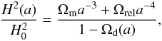 (1)a simple, analytic expression for Ωd(a) enables us to compute many astrophysical quantities analytically. Here
  is the fractional energy density of relativistic neutrinos and photons today,
  is the matter fractional energy density.
The form of parameterization, namely 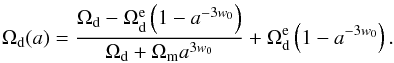 (2)Here Ωd = 1 − Ωm is the present dark energy density, is the asymptotic early dark energy density, and w0 is the present dark energy equation of state (EOS). In addition to the matter density, the two parameters are and w0. The standard formula for the EOS, w = −1/(3 [1 − Ωd(a)] ) dlnΩd(a)/dlna, can not be simplified in this model. The deceleration parameter can be derived by, q(z) = (1 + z)H-1dH/dz − 1.
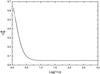 |
Fig. 1 The early dark energy density |
In Fig. 1 we plot the dark energy density as a function of redshift with  , w0 = −1.08 and
  . In Fig. 2 we show the equation of state as a function of redshift. We can see that the dark energy density does not act to accelerate expansion at early times, and in fact w → 0. In Fig. 3, we plot the deceleration parameter q(z) as a function of redshift. The transition redshift is zT = 0.62.
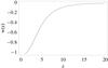 |
Fig. 2 The equation of state w(z) of early dark energy as a function of redshift with |
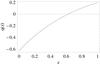 |
Fig. 3 The evolution of deceleration parameter q(z) with |
The growth of perturbations is strongly affected by the unclustered early dark energy. We introduce the linear perturbation growth theory as follow. To linear order of perturbation, at large scales the matter density perturbation δ = δρm/ρm satisfies the simple equation: 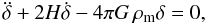 (3)where ρm is the matter energy density. In terms of the growth factor f = dlnδ/dlna, the matter density perturbation Eq. (3) becomes
 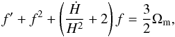 (4)where f′ = df/dlna. The solution of the equation can be approximated as
  (Peebles 1980; Fry 1985; Lightman & Schechter 1990; Wang & Steinhardt 1998) and the growth index γ can be obtained for some general models. For a dynamical dark energy model with slowly varying w and zero curvature, the approximation f(z) = Ω(z)γ was given in Wang & Steinhardt (1998). For more general dynamical dark energy models in flat space, it was found that γ = 0.55 + 0.05 [1 + w(z = 1)] with w > − 1 and γ = 0.55 + 0.02 [1 + w(z = 1)] with w < − 1 (Linder 2005; Linder & Cahn 2007). For the flat DGP model, γ = 11/16 (Linder & Cahn 2007). In non-flat case, an approximation for the growth factor
 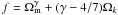 is given in Gong et al. (2009). More recently Linder (2009) shows that the numerical solution of Eq. (4) can be approximated as
 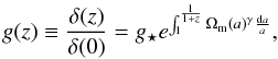 (5)where g ⋆ is the calibration parameter of the growth behavior at early times. Enhanced growth involves g ⋆ > 1, and any deviation from g ⋆ = 1 signals a nonstandard early universe behavior (Linder 2009). The calibration parameter is important in early dark energy cosmology. In Fig. 4, we show the normalized growth of Eq. (5) and the numerical result of Eq. (3). The dashed line shows the numerical result of Eq. (3) and the solid line shows result from Eq. (5) with
  , w0 = −1.04, , g ⋆ = 0.98 and γ = 6/11. These parameter are obtained from latest observational data constraint. We show that the numerical solution of Eq. (4) is well consistent with the approximate result (Eq. (5)).
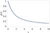 |
Fig. 4 The numerically obtained solution of Eq. (3) and the normalized growth of Eq. (5). The dashed line shows the numerical result of Eq. (3) and the solid line shows result from Eq. (5) with |
3. Observational data and analysis methods
3.1. Type Ia supernovae (SNe Ia)
First, we use the Union2 compilation of 557 type Ia SNe (Amanullah et al. 2010). The theoretical distance modulus is defined as  (6)where μ0 ≡ 42.38 − 5log 10h with h is the Hubble constant H0 in units of 100 km/s/Mpc, and
  (7)is the Hubble-free luminosity distance H0dL (here dL is the physical luminosity distance) in a spatially flat FRW universe, and here θ denotes the model parameters. The χ2 for the SNe Ia data is
 ![Mathematical equation: \begin{equation} \chi^2_{\rm SN}({\bf\theta})=\sum\limits_{i=1}^{557}{[\mu_{\rm obs}(z_i)-\mu_{\rm th}(z_i)]^2\over \sigma_i^2},\label{ochisn} \end{equation}](/articles/aa/full_html/2012/07/aa19348-12/aa19348-12-eq60.png) (8)where μobs(zi) and σi are the observed value and the corresponding 1σ error of distance modulus for each supernova, respectively. The parameter μ0 is a nuisance parameter but it is independent of the data and the dataset. Following Nesseris & Perivolaropoulos (2005), the minimization with respect to μ0 can be made trivially by expanding the χ2 of Eq. (8) with respect to μ0 as
(8)where μobs(zi) and σi are the observed value and the corresponding 1σ error of distance modulus for each supernova, respectively. The parameter μ0 is a nuisance parameter but it is independent of the data and the dataset. Following Nesseris & Perivolaropoulos (2005), the minimization with respect to μ0 can be made trivially by expanding the χ2 of Eq. (8) with respect to μ0 as  (9)where
 ![Mathematical equation: \begin{eqnarray} A({\bf\theta})&=&\sum\limits_{i=1}^{557}{[\mu_{\rm obs}(z_i)-\mu_{\rm th}(z_i;\mu_0=0,{\bf\theta})]^2\over \sigma_i^2}, \\ B({\bf\theta})&=&\sum\limits_{i=1}^{557}{\mu_{\rm obs}(z_i)-\mu_{\rm th}(z_i;\mu_0=0,{\bf\theta})\over \sigma_i^2}, \\ C&=&\sum\limits_{i=1}^{557}{1\over \sigma_i^2}\cdot \end{eqnarray}](/articles/aa/full_html/2012/07/aa19348-12/aa19348-12-eq65.png) Evidently, Eq. (8) has a minimum for μ0 = B/C at
Evidently, Eq. (8) has a minimum for μ0 = B/C at  (13)Since
  , instead minimizing
  one can minimize
  which is independent of the nuisance parameter μ0.
3.2. Cosmic microwave background
In order to implement the WMAP7 data, we use the distance priors from (Komatsu et al. 2011). It has been shown that the constraints on cosmological parameters from WMAP7 distance priors are good agreement with the full MCMC results (Komatsu et al. 2011). We use three fitting parameters R, la and z ∗ . The acoustic scale la is  (14)where the redshift z ∗ is given by (Hu & Sugiyama 1996)
 ![Mathematical equation: \begin{eqnarray} \label{zstareq} z_*&=&1048\left[1+0.00124\left(\Omega_{\rm b} h^2\right)^{-0.738}\right]\left[1+g_1\left(\Omega_{\rm m} h^2\right)^{g_2}\right]\nonumber\\ &=&1091.3\pm 0.91, \\ g_1&=&\frac{0.0783(\Omega_{\rm b} h^2)^{-0.238}}{1+39.5(\Omega_{\rm b} h^2)^{0.763}},\quad g_2=\frac{0.560}{1+21.1(\Omega_{\rm b} h^2)^{1.81}}, \end{eqnarray}](/articles/aa/full_html/2012/07/aa19348-12/aa19348-12-eq75.png) and rs(z ∗ ) is the comoving sound horizon at z ∗ . We must notice that comoving sound horizon changes as
and rs(z ∗ ) is the comoving sound horizon at z ∗ . We must notice that comoving sound horizon changes as  . The shift parameter
  (17)The χ2 of the CMB data is constructed as
  , where
 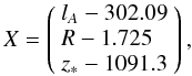 (18)and the inverse covariance matrix is given by (Komatsu et al. 2011)
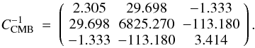
3.3. Baryon acoustic peak from SDSS and 2dFGRS
It is well known that the acoustic peaks in CMB anisotropy power spectrum can be used to determine the properties of perturbations and to constrain cosmological parameters and dark energy. The acoustic peaks occur because the cosmic perturbations excite sound waves in the relativistic plasma of the early universe. Because the universe has a fraction of baryons, the acoustic oscillations in the relativistic plasma will be imprinted onto the late-time power spectrum of the nonrelativistic matter (Eisenstein & Hu 1998). The acoustic signatures in the large-scale clustering of galaxies can also be used to constrain cosmological parameters and dark energy. The detection of a peak in the correlation function of luminous red galaxies in the 2dFGRS and Sloan Digital Sky Survey. This peak can provide a“standard ruler" with which to constrain cosmological parameters.
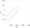 |
Fig. 5 Constraints on |
To use the baryon acoustic oscillations (BAO) measurement from the SDSS and 2dFGRS data, we define (Percival et al. 2010) 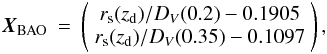 (19)and using the inverse covariance matrix (Percival et al. 2010)
 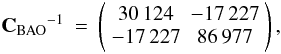 (20)we find the contribution of BAO to χ2 as
  (21)where the effective distance is
 ![Mathematical equation: \begin{equation} \label{dvdef} D_V(z)=\left[\frac{d_{\rm L}^2(z)}{(1+z)^2}\frac{z}{H(z)}\right]^{1/3}\cdot \end{equation}](/articles/aa/full_html/2012/07/aa19348-12/aa19348-12-eq88.png) (22)The effect of early dark energy is a change in DV(z), such as
(22)The effect of early dark energy is a change in DV(z), such as  and
and  (Doran et al. 2007). The redshift zd is fitted with the formulae (Eisenstein & Hu 1998)
 ![Mathematical equation: \begin{equation} \label{zdfiteq} z_{\rm d}=\frac{1291\left(\Omega_{\rm m} h^2\right)^{0.251}}{1+0.659\left(\Omega_{\rm m} h^2\right)^{0.828}}\left[1+b_1\left(\Omega_{\rm b} h^2\right)^{b_2}\right], \end{equation}](/articles/aa/full_html/2012/07/aa19348-12/aa19348-12-eq93.png) (23)
(23)![Mathematical equation: \begin{eqnarray} \label{b1eq} b_1&=&0.313\left(\Omega_{\rm m} h^2\right)^{-0.419}\left[1+0.607\left(\Omega_{\rm m} h^2\right)^{0.674}\right],\nonumber\\ b_2&=&0.238\left(\Omega_{\rm m} h^2\right)^{0.223}, \end{eqnarray}](/articles/aa/full_html/2012/07/aa19348-12/aa19348-12-eq94.png) (24)and the comoving sound horizon is
(24)and the comoving sound horizon is  (25)where the sound speed
 ![Mathematical equation: \hbox{$c_{\rm s}(z)=1/\sqrt{3[1+\bar{R_{\rm b}}/(1+z)}]$}](/articles/aa/full_html/2012/07/aa19348-12/aa19348-12-eq96.png) ,
,  . The CMB temperature is Tcmb = 2.725 K.
4. Observational constraints on early dark energy
For Gaussian distributed measurements, the likelihood function L ∝ e − χ2/2, with  (26)We also marginalize nuisance parameters H0 and Ωbh2. The latest Hubble constant is H0 = 74.2 ± 3.6 km s-1 Mpc (Riess et al. 2009). The baryon density is Ωbh2 = 0.02265 ± 0.00059 (Komatsu et al. 2011). The likelihood for the parameters (Ωm, w0, ) in the model is computed by minimizing the χ2. Our program randomly chooses values for the above parameters, evaluate χ2.
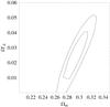 |
Fig. 6 The 1σ, 2σ confidence regions for Ωm versus |
By fitting the early dark energy model using combined data, we find  ,
,  ,
,  , and
, and  . Figure 5 shows constraints on the
  plane. Figure 6 shows constraints on the
  plane. At 2σ confidence level, we find that the fractional dark energy density
  .
.
σ8 values and growth rates with 1σ error bars from which we derived the linear growth factors used in our analysis.
4.1. High-redshift probes
In order to make tight constraints on early dark energy models, we must add high-redshift probes, such as GRBs and linear growth factors data. GRBs can be detectable out to very high redshifts. The farthest burst detected so far is GRB 090429B, which is at z = 9.4 (Cucchiara et al. 2011). GRBs could in principle serve as such high redshift standardizable candles (Dai et al. 2004; Wang 2008; Wang et al. 2007, 2009; Basilakos & Perivolaropoulos 2008; Izzo et al. 2009; Schaefer 2007). We use the latest 116 GRBs sample summarized in Wang et al. (2011). We use the method shown in Wang & Dai (2011) to calibrate the GRB luminosity relations. First we fit the cosmographic parameters using the Union2 sample. Then we deduce the distance moduli of GRBs at z ≤ 1.4. Last using these deduced distance moduli and the redshifts of corresponding GRBs, we calibrate four GRB luminosity correlations. We assume these relations do not evolve with redshift and are valid at z > 1.40, which is also confirmed by Wang et al. (2011). The luminosity or energy of GRB can be calculated. So the luminosity distances and distance modulus can be obtained. After obtaining the distance modulus of each burst using one of these relations, we use the same method as Schaefer (2007) to calculate the real distance modulus,  (27)where the summation runs from 1–4 over the relations with available data, μi is the best estimated distance modulus from the ith relation, and σμi is the corresponding uncertainty. The uncertainty of the distance modulus for each burst is
 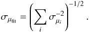 (28)The \verbatimmathformule{!/chi!*2} valueis
 ![Mathematical equation: \begin{equation} \chi^{2}_{\rm GRB}=\sum_{i=1}^{N} \frac{[\mu_{i}(z_{i})-\mu_{{ fit},i}]^{2}}{\sigma_{\mu_{{\rm fit},i}}^{2}}, \end{equation}](/articles/aa/full_html/2012/07/aa19348-12/aa19348-12-eq127.png) (29)where μfit,i and σμfit,i are the fitted distance modulus and its error. This method is almost model-independent.
(29)where μfit,i and σμfit,i are the fitted distance modulus and its error. This method is almost model-independent.
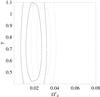 |
Fig. 7 Solid contours: the 1σ, 2σ confidence regions for γ versus |
We also use the linear growth factor data in Table 1. There are 20 data points at a redshift range (0.15, 3.8) in Table 1. We include the growth rate data from WiggleZ Dark Energy Survey (Blake et al. 2011). Balke et al. (2011) presented fits for the growth rate of structure using redshift-space distortions in the 2D power spectrum. These fits included a full exploration of the systematic errors arising from the assumption of redshift-space distortion models based on perturbation theory techniques, fitting formulae calibrated by N-body simulations, and empirical models. After including GRBs and linear growth factor data, we find  ,
,  , and
, and  with
with  . In Fig. 7, we show the confidence regions for γ and from 1σ to 2σ. Dotted contours show constraints from SN+CMB+BAO. The solid contours are obtained by adding GRBs and linear growth factors data. By minimizing
  , we find
  at 2σ confidence level. After including high-redshift GRBs, the constraints can be tightened to
  at 2σ confidence level.
4.2. Growth index
In this section, we put constraint on the growth factor. The observational probe of the growth function δ(z) is the redshift dependence of the rms mass fluctuation σ8(z) defined by 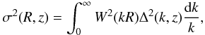 (30)with
  with R = 8h-1Mpc and Pδ(k,z) the mass power spectrum at redshift z. The function σ8(z) is
  (33)which implies
 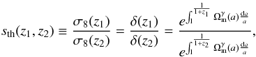 (34)where we use Eq. (5). The currently available data points σ8(zi) originate from the observed redshift evolution of the flux power spectrum of Lyα forest (Viel et al. 2004; Viel & Haehnelt 2006). These data points are shown in Table 1 along with the corresponding references. The currently available data for the parameters f at various redshifts are also shown in Table 1 below.
Using the data of Table 1 we construct the corresponding  defined as
 ![Mathematical equation: \begin{eqnarray} \chi_{\gamma}^2 (\gamma)&=&\sum_i \left[\frac{s_{\rm obs}(z_i,z_{i+1})-s_{\rm th}(z_i,z_{i+1})}{\sigma_{s_{\rm obs,i}}}\right]^2\nonumber\\ &&+\sum_i\left[\frac{f_{\rm obs}(z_i)-f_{\rm th}(z_i)}{\sigma_{f_{\rm obs,i}}}\right]^2\nonumber\\ &&+\sum_i\left[\frac{f_{\rm obs}\sigma_8(z_i)-f_{\rm th}\sigma_8(z_i)}{\sigma_{\sigma_8f_{\rm obs,i}}}\right]^2\label{chi2s} \end{eqnarray}](/articles/aa/full_html/2012/07/aa19348-12/aa19348-12-eq148.png) (35)where σsobs,i is derived by error propagation from the corresponding 1σ errors of σ8(zi) and σ8(zi + 1) while sth(zi,zi + 1) is defined in Eq. (34).
(35)where σsobs,i is derived by error propagation from the corresponding 1σ errors of σ8(zi) and σ8(zi + 1) while sth(zi,zi + 1) is defined in Eq. (34).
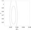 |
Fig. 8 The 1σ, 2σ confidence regions for γ versus |
Using the data points in Table 1 and the datasets above, we find 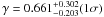 with
with  by minimizing
  . This result is a little different from (Xia & Viel 2009; Nesseris & Perivolaropoulos 2008; Di Porto & Amendola 2008), because we have used the new parametrization of early dark energy and latest data set. In Fig. 8, we show the confidence contours of γ vs. . After including high-redshift GRB data, the growth index becomes
  . We must notice that the fobs in Table 1 were derived by assuming ΛCDM with Ωm = 0.30 when converting redshifts to distances for the power spectra. So their use to test models largely different from ΛCDM might be unreliable, as discussed in Nesseris & Perivolaropoulos (2008). We can use these data when small deviations from flat ΛCDM with Ωm = 0.30 are considered. We believe that we are in such a situation in this paper. As mentioned above, the key problem is the redshift-distance relation. In Fig. 9, we show the relation between z and H0r(z), where r(z) is the comoving distance. The solid line is the H0r(z) in flat ΛCDM with Ωm = 0.3 and dashed line is the H0r(z) in EDE with best fitted parameters (Ωm = 0.29,
  , w0 = −1.04). The redshift-distance relation in EDE model has small deviations from ΛCDM. So we can use the data of Table 1 in this early dark energy model.
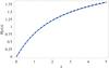 |
Fig. 9 The solid line shows the H0r(z) in flat ΛCDM with Ωm = 0.3 and dashed line shows the H0r(z) in EDE with best fitted parameters (Ωm = 0.29, |
5. Conclusions and discussion
In this paper we present constraints on a particular early dark energy model using the latest observations. We use the early dark energy model proposed by Doran & Robbers (2006). We find that the fractional dark energy density at 2σ confidence level, using the latest Union SNe Ia, the WMAP seven-year data and baryon acoustic oscillations measurement from the SDSS and 2dFGRS. If we add high-redshift GRBs and linear growth factors data from Lyα forest data, the constraint is improved to at 2σ confidence level. The constraint on the growth rate index γ is using the SNe Ia, CMB, BAO and linear growth factor data. After including high-redshift GRB data, the growth index is . This result is clearly consistent at 1σ with the value predicated by ΛCDM.
High-redshift probes, such as GRBs and Lyα are important in constraining early dark energy models. In this paper, we calibrate the luminosity relations of GRBs by SNe Ia using cosmographic parameters. The derived distance modulus of GRBs are model-independent. These measurements of growth factor, summarized in Table 1, have been obtained in the framework of pure ΛCDM model and are valid only when small deviations from this model are considered. Because the references of Table 1 have assumed ΛCDM with Ωm = 0.30 when converting redshifts to distances for the power spectra. In this early dark energy model with the best fitted parameters, the redshift-distance relation is small derivation from ΛCDM with Ωm = 0.30. This can be seen from Fig. 9. So the growth factor data are valid in this early dark energy model.
Early dark energy significantly affects the size of the sound horizon. The sound horizon is a crucial quantity because it is employed as a standard ruler in the baryon acoustic oscillation technique for probing cosmology. If the standard ruler is miscalibrated due to ignore early dark energy, the cosmological parameters will be biased. Early dark energy also has been shown to influence the growth of cosmic structures, to change the age of the universe, to have an effect on CMB physics. So probing the early dark energy using future observational data is important.
Acknowledgments
This work is supported by the National Natural Science Foundation of China (grant 11103007) and China Postdoctoral Science Foundation funded projects (grants 20100481117 and 201104521).
References
- Alam, U. 2010, ApJ, 714, 1460 [NASA ADS] [CrossRef] [Google Scholar]
- Alam, U., Lukic, Z., & Bhattacharya, S. 2011, ApJ, 727, 87 [NASA ADS] [CrossRef] [Google Scholar]
- Amanullah, R., Lidman, C., Rubin, D., et al. 2010, ApJ, 716, 712 [NASA ADS] [CrossRef] [Google Scholar]
- Basilakos, S., & Perivolaropoulos, L. 2008, MNRAS, 391, 411 [NASA ADS] [CrossRef] [Google Scholar]
- Blake, C., Brough, S., Colless, M., et al. 2011, MNRAS, 415, 2876 [NASA ADS] [CrossRef] [Google Scholar]
- Calabrese, E. R., de Putter, D., Huterer, et al. 2011a, Phys. Rev. D, 83, 023011 [NASA ADS] [CrossRef] [Google Scholar]
- Calabrese, E. D., Huterer, E. V., Linder, et al. 2011b, Phys. Rev. D, 83, 123504 [NASA ADS] [CrossRef] [Google Scholar]
- Caldwell, R. R. 2002, Phys. Lett. B, 545, 23 [NASA ADS] [CrossRef] [Google Scholar]
- Cucchiara, A., Levan, A. J., Fox, D. B., et al. 2011, ApJ, 736, 7 [NASA ADS] [CrossRef] [Google Scholar]
- Dai, Z. G., Liang, E. W., & Xu, D. 2004, ApJ, 612, L101 [NASA ADS] [CrossRef] [Google Scholar]
- da Angela, J., Shanks, T., Croom, S. M., et al. 2008, MNRAS, 383, 565 [NASA ADS] [CrossRef] [Google Scholar]
- de Putter, R., Zahn, O., & Linder, E. V. 2009, Phys. Rev. D, 79, 065033 [NASA ADS] [CrossRef] [Google Scholar]
- Di Porto, C., & Amendola, L. 2008, Phys. Rev. D, 77, 083508 [NASA ADS] [CrossRef] [Google Scholar]
- Doran, M., & Robbers, G. 2006, JCAP, 0606, 026 [Google Scholar]
- Doran, M., Stern, S., & Thommes, E. 2007, JCAP, 04, 015 [CrossRef] [Google Scholar]
- Eisenstein, D. J., & Hu, W. 1998, ApJ, 496, 605 [NASA ADS] [CrossRef] [Google Scholar]
- Eisenstein, D. J., Zehavi, I., Hogg, D. W., et al. 2005, ApJ, 633, 560 [NASA ADS] [CrossRef] [Google Scholar]
- Feng, B., Wang, X. L., & Zhang, X. M. 2005, Phys. Lett. B, 607, 35 [NASA ADS] [CrossRef] [Google Scholar]
- Francis, M. J., Lewis, G. F., & Linder, E. V. 2008, MNRAS, 393, L31 [NASA ADS] [Google Scholar]
- Fry, J. N. 1985, Phys. Lett. B, 158, 211 [NASA ADS] [CrossRef] [Google Scholar]
- Gong, Y. G., Ishak, M., & Wang, A. Z. 2009, Phys. Rev. D, 80, 023002 [NASA ADS] [CrossRef] [Google Scholar]
- Grossi, M., & Springel, V. 2009, MNRAS, 354, 1509 [Google Scholar]
- Hawkins, E., Maddox, S., Cole, S., et al. 2003, MNRAS, 346, 78 [Google Scholar]
- Hollenstein, L., et al. 2009, JCAP, 0904, 012 [NASA ADS] [CrossRef] [Google Scholar]
- Hu, W., & Sugiyama, N. 1996, ApJ, 471, 542 [NASA ADS] [CrossRef] [Google Scholar]
- Izzo, L., Capozziello, S., Covone, G., & Capaccioli, M. 2009 [arXiv:0906.4888] [Google Scholar]
- Komatsu, E., Smith, K. M., Dunkley, J., et al. 2011, ApJS, 192, 18 [NASA ADS] [CrossRef] [Google Scholar]
- Liang, N., et al. 2008, ApJ, 685, 354 [NASA ADS] [CrossRef] [Google Scholar]
- Lightman, A. P., & Schechter, P. L. 1990, ApJ, 74, 831 [Google Scholar]
- Linder, E. V. 2005, Phys. Rev. D, 72, 043529 [NASA ADS] [CrossRef] [MathSciNet] [Google Scholar]
- Linder, E. V. 2006, Astropart. Phys., 26, 16 [NASA ADS] [CrossRef] [Google Scholar]
- Linder, E. V. 2009, Phys. Rev. D, 79, 063519 [NASA ADS] [CrossRef] [Google Scholar]
- Linder, E. V., & Cahn, R. N. 2007, Astropart. Phys., 28, 481 [NASA ADS] [CrossRef] [Google Scholar]
- Linder, E. V., & Robbers, G. 2008, JCAP, 06, 004 [NASA ADS] [CrossRef] [Google Scholar]
- McDonald, P., Seljak, U., Cen, R., et al. 2005, ApJ, 635, 761 [NASA ADS] [CrossRef] [Google Scholar]
- Mota, D. F. 2008, JCAP, 09, 006 [Google Scholar]
- Nesseris, S., & Perivolaropoulos, L. 2005, Phys. Rev. D, 72, 123519 [NASA ADS] [CrossRef] [Google Scholar]
- Nesseris, S., & Perivolaropoulos, L. 2008, Phys. Rev. D, 77, 023504 [NASA ADS] [CrossRef] [Google Scholar]
- Peebles, P. J. E. 1980, The Large-Scale Structure of the Universe (Princeton, New Jersey: Princeton University Press). [Google Scholar]
- Peebles, P. J. E., & Ratra, B. 2003, Rev. Mod. Phys., 75, 559 [NASA ADS] [CrossRef] [MathSciNet] [Google Scholar]
- Percival, W. J., Reid, B. A., Eisenstein, D. J., et al. 2010, MNRAS, 401, 2148 [NASA ADS] [CrossRef] [Google Scholar]
- Perlmutter, S., Aldering, G., Goldhaber, G., et al. 1999, ApJ, 517, 565 [NASA ADS] [CrossRef] [Google Scholar]
- Ratra, B., & Peebles, P. J. E. 1988, Phys. Rev. D, 37, 3406 [NASA ADS] [CrossRef] [MathSciNet] [Google Scholar]
- Reichardt, C. L., de Putter, R., Zahn, O., & Hou, Z. 2012, ApJ, 749, L9 [NASA ADS] [CrossRef] [Google Scholar]
- Riess, A. G., Filippenko, A. V., Challis, P., et al. 1998, AJ, 116, 1009 [NASA ADS] [CrossRef] [Google Scholar]
- Riess, A. G., Macri, L., Casertano, S., et al. 2009, ApJ, 699, 539 [NASA ADS] [CrossRef] [Google Scholar]
- Ross, N. P., et al. 2007, MNRAS, 381, 57 [Google Scholar]
- Schaefer, B. E. 2007, ApJ, 660, 16 [NASA ADS] [CrossRef] [Google Scholar]
- Silveira, V., & Waga, I. 1994, Phys. Rev. D, 50, 4890 [NASA ADS] [CrossRef] [Google Scholar]
- Tegmark, M., et al. 2006, Phys. Rev. D, 74, 123507 [Google Scholar]
- Verde, L., et al. 2002, MNRAS, 335, 432 [Google Scholar]
- Vitagliano, V., Xia, J. Q., Liberati, S., & Viel, M. 2010, JCAP, 03, 005 [NASA ADS] [CrossRef] [Google Scholar]
- Viel, M., & Haehnelt, M. G. 2006, MNRAS, 365, 231 [NASA ADS] [CrossRef] [Google Scholar]
- Viel, M., Haehnelt, M. G., & Springel, V. 2004, MNRAS, 354, 684 [NASA ADS] [CrossRef] [Google Scholar]
- Wang, Y. 2008, Phys. Rev. D, 78, 123532 [NASA ADS] [CrossRef] [Google Scholar]
- Wang, F. Y., & Dai, Z. G. 2011, A&A, 536, A96 [NASA ADS] [CrossRef] [EDP Sciences] [Google Scholar]
- Wang, L., & Steinhardt, P. J. 1998, ApJ, 508, 483 [NASA ADS] [CrossRef] [Google Scholar]
- Wang, F. Y., Dai, Z. G., & Zhu, Z. H. 2007, ApJ, 667, 1 [NASA ADS] [CrossRef] [Google Scholar]
- Wang, F. Y., Dai, Z. G., & Qi, S. 2009, RA&A, 9, 547 [CrossRef] [Google Scholar]
- Wang, F. Y., Qi, S., & Dai, Z. G. 2011, MNRAS, 415, 3423 [NASA ADS] [CrossRef] [Google Scholar]
- Weinberg, S. 1989, Rev. Mod. Phys., 61, 1 [NASA ADS] [CrossRef] [MathSciNet] [Google Scholar]
- Wetterich, C. 1988, Nucl. Phys. B, 302, 645 [NASA ADS] [CrossRef] [Google Scholar]
- Wetterich, C. 2004, Phys. Lett. B, 594, 17 [NASA ADS] [CrossRef] [Google Scholar]
- Xia, J.-Q., & Viel, M. 2009, JCAP, 04, 002 [NASA ADS] [CrossRef] [Google Scholar]
- Xia, J. Q., Vitagliano, V., Liberati, S., & Viel, M. 2012, Phys. Rev. D, 85, 043520 [NASA ADS] [CrossRef] [Google Scholar]
All Tables
σ8 values and growth rates with 1σ error bars from which we derived the linear growth factors used in our analysis.
All Figures
|
Fig. 1 The early dark energy density |
| In the text | |
|
Fig. 2 The equation of state w(z) of early dark energy as a function of redshift with |
| In the text | |
|
Fig. 3 The evolution of deceleration parameter q(z) with |
| In the text | |
|
Fig. 4 The numerically obtained solution of Eq. (3) and the normalized growth of Eq. (5). The dashed line shows the numerical result of Eq. (3) and the solid line shows result from Eq. (5) with |
| In the text | |
|
Fig. 5 Constraints on |
| In the text | |
|
Fig. 6 The 1σ, 2σ confidence regions for Ωm versus |
| In the text | |
|
Fig. 7 Solid contours: the 1σ, 2σ confidence regions for γ versus |
| In the text | |
|
Fig. 8 The 1σ, 2σ confidence regions for γ versus |
| In the text | |
|
Fig. 9 The solid line shows the H0r(z) in flat ΛCDM with Ωm = 0.3 and dashed line shows the H0r(z) in EDE with best fitted parameters (Ωm = 0.29, |
| In the text | |
Current usage metrics show cumulative count of Article Views (full-text article views including HTML views, PDF and ePub downloads, according to the available data) and Abstracts Views on Vision4Press platform.
Data correspond to usage on the plateform after 2015. The current usage metrics is available 48-96 hours after online publication and is updated daily on week days.
Initial download of the metrics may take a while.