| Issue |
A&A
Volume 543, July 2012
|
|
|---|---|---|
| Article Number | A7 | |
| Number of page(s) | 6 | |
| Section | The Sun | |
| DOI | https://doi.org/10.1051/0004-6361/201219266 | |
| Published online | 20 June 2012 | |
The solar differential rotation in the 18th century
Leibniz-Institut für Astrophysik Potsdam (AIP), An der Sternwarte 16, 14482 Potsdam, Germany
e-mail: This email address is being protected from spambots. You need JavaScript enabled to view it.
Received: 22 March 2012
Accepted: 7 May 2012
Abstract
The sunspot drawings of Johann Staudacher of 1749–1799 were used to determine the solar differential rotation in that period. These drawings of the full disk lack any indication of their orientation. We used a Bayesian estimator to obtain the position angles of the drawings, the corresponding heliographic spot positions, a time offset between the drawings and the differential rotation parameter δΩ, assuming the equatorial rotation period is the same as today. The drawings are grouped in pairs, and the resulting marginal distributions for δΩ were multiplied. We obtain δΩ = −0.048 ± 0.025 d-1 (−2.75 °/d) for the entire period. There is no significant difference to the value of the present Sun. We find an (insignificant) indication for a change of δΩ throughout the observing period from strong differential rotation, δΩ ≈ −0.07 d-1, to weaker differential rotation, δΩ ≈ −0.04 d-1.
Key words: Sun: rotation / sunspots / methods: statistical
© ESO, 2012
1. Introduction
The solar activity cycle is the result of an oscillatory magnetic dynamo in the interior of the Sun. Practically all available dynamo models for the Sun require a differential rotation for part of the amplification of the magnetic fields. Today’s solar differential rotation is known from helioseismology with fairly high precision down to the bottom of the convection zone.
The rotation period of the pole is considerably longer than the one at the equator. Balthasar et al. (1986) determined the differential rotation from the rotational motion of sunspots. Although sunspots provide no information on the rotational period at the pole, we can extrapolate certain profiles of the rotation to the pole and obtain a polar rotation period, which is 25% longer than the equatorial one. While the profile in Balthasar et al. (1986) runs from about 24.7 d at the equator to 31 d at the pole, the rotation profile obtained from helioseismology runs from about 25.2 d to about 38 d (Korzennik & Eff-Darwich 2011). It is a typical feature of solar activity that sunspot rotation periods are slightly shorter than the rotation period of the photosphere (Benevolenskaya et al. 1999).
Several simulations of the dynamo process included the modulation of the differential rotation as a source of the solar cycle variability. Many global dynamo solutions are kinematic solution, which do not integrate an equation of motion over time. Small-scale motions are comprised in a source term that usually contains a nonlinearity that mimicks the back-reaction of the magnetic fields on the flows (α-effect and α-quenching). Typically, the source term is significantly diminished for magnetic fields B stronger than the equipartition field strength defined by  , where μ0 and ρ are the magnetic permeability and the density, respectively, and u′ is the typical turbulent velocity. It is, however, not only the feedback to the small-scale motions but also the back-reaction on the large-scale flows, in particular the differential rotation, which introduces a non-linearity to the dynamo system.
The fields generated in the dynamo process exert Lorentz forces, which modulate the differential rotation. This was studied by Malkus & Proctor (1975) who found highly nonlinear behaviour and complex time-series. These authors applied the Lorentz force from the large-scale magnetic field to the large-scale motion (differential rotation). In a refined attempt, Küker et al. (1999) also included the back-reaction of the generated large-scale field on the turbulent redistribution of angular momentum (Λ-effect and Λ-quenching). They found time-variations of the dynamo solution that are very reminiscent of grand minima in the solar activity time-series, e.g. the Maunder minimum.
These models are of course accompanied by amplitude variations of the differential rotation. It will therefore be extremely interesting to measure the differential rotation at various instances of the 400-year record of telescopic sunspot observations.
An attempt to determine the differential rotation during the period of the Maunder minimum indeed indicated a differential rotation that was stronger in the period of 1701 − 1719 than on the present Sun (Ribes & Nesme-Ribes 1993). The whole rotation period of the Sun appeared to be shorter, with a slow-down at the turn of the 17th century.
We investigated the period of 1749–1799 with the attempt to determine the differential rotation of the Sun in a thorough statistical analysis.
2. Data set
We used the drawings of the full solar disk made by Johann Caspar Staudacher in Nuremberg in the second half of the 18th century as described by Arlt (2008). All drawings were made employing the projection method which can be deduced from the orientations of the drawings of solar eclipses. The drawings lack any indication of the orientation. The sunspot positions determined by Arlt (2009) were obtained by matching the solar rotation profile with the spots in adjacent drawings. Here we cannot take the sunspot positions obtained by Arlt (2009) into account, since these employed the rotation profile by Balthasar et al. (1986) to find the position angles of the solar disks, and do not allow an independent determination of the differential rotation.
The entire set of sunspot drawings by Staudacher was examined in suitable pairs, which contain several apparently identical spots in both images (Fig. 1). It is obvious that we have to compile a considerable number N of pairs in a sample to determine the differential rotation. Apart from the intrinsic plotting errors in the drawings, additional errors may occur when spots in adjacent drawings were associated with each other, while they were actually not related.
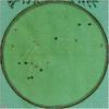 |
Fig. 1 Association of spots in the two superimposed images of 1761 June 23 (spots coloured in green) and 1761 June 24 (spots coloured in red). The difference in position angles determined by rotational matching is 29.8°. |
3. Data analysis
3.1. Defining the unknowns
The entire 999 individual drawings of the solar disk were inspected manually for suitable pairs of drawings. Drawings with less than three spots were omitted, since they do not deliver enough information to statistically determine of the free parameters. A final set of 288 pairs were found with at least three spots in common. Several drawings were used twice if the combinations with the preceding and the succeeding drawings provided suitable pairs. As in Arlt (2009), the drawings were cut out of the photos by defining the left, right, lower, and upper edge of the solar disk on the screen. Parts of any elliptical deformations can be compensated for in this way. The actual spot pairs were picked in an image that contained the two superimposed drawings, which were now perfectly circular and slightly magnified. The scale in the disk centre is 0.12° per pixel in heliographic coordinates. Using the rotation profile by Balthasar et al. (1986), we estimated the expected displacements of spots. After one day a spot at 10° heliographic latitude becomes displaced by 0.63° in longitude against a spot at 30° latitude. This displacement corresponds to about 5 pixels and should be measurable. Obviously, it is difficult to detect the differential rotation signal in the observations because of these quite small displacements. It is the statistical multitude of drawings that delivers a measurement of the differential rotation with reasonable accuracy.
In any ith pair of drawings, we measured the cartesian coordinates  and
and  of ni spots visible in both drawing (1) and drawing (2), normalised in the solar radius, i.e. taking values between − 1 and 1. We assumed that the longitudes λi,j, the latitudes bi,j, and the two position angles of the drawings pi, qi are unknown, where j counts from one to the number of common spots ni. We also assumed that the profile of the angular velocity can be expressed in terms of
 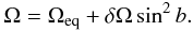 (1)In order to place a given spot at the same longitude in a pre-defined rotating frame, we need to know the precise times of the two drawings. Unfortunately, these are not always provided. Even when there are notes about the times, they are hardly more precise than to the full hour. In principle, we can also keep the time difference Δti between the two drawings unknown. Note, however, that the three quantities Ωeq,i, δΩi, and Δti are highly correlated. Any change in Δti can always be compensated for by a corresponding change in Ωeq,i.
In the same way, if the spots are on similar latitudes, the angular velocity Ωeq,i and the differential rotation parameter δΩi are highly correlated, since a lower equatorial velocity can be compensated for by a larger differential rotation parameter. We have a few options to reduce this redundancy:
-
we may assume that the times given by Staudacher are sufficientlyaccurate andfixe Δti. The parameters Ωeq,i, δΩi have to reproduce the longitudinal motion of the spots alone;
-
we may assume that the equatorial rotation period Ωeq of the Sun has not changed and fix it at today’s value. If this cannot explain the spots’ longitudinal displacement, Δti will compensate for this. Remaining discrepancies can be mediated by δΩi;
-
we may assume that the total angular momentum of the Sun has not changed since Staudacher. If we assume that the shape of the internal rotation profile has not changed (except its amplitude), and if we assume that we know this profile precisely, we can find a relation for δΩi(Ωeq,i). Hence, only Ωeq,i and Δti are the unknowns.
The first option is the most natural choice but turned out to be problematic, since the times given by Staudacher appear to be rough estimates only. There is also a considerable number of drawings for which no time is given except the date. Excluding these would leave us with too few pairs to obtain a meaningful result. The last option appears to be the most physical one since it is highly unlikely that the total angular momentum has changed over 250 yr. The solar wind carries away only about 1030 g cm2 s-2 sr-1 (Pizzo et al. 1983). In 250 yr this is less than 10-8 A⊙, where A⊙ is the total angular momentum of the Sun of about A⊙ = 2 × 1048 g cm2 s-1 (e.g. Komm et al. 2003). The problem with this approach, however, is that fixing the total angular momentum does not fix the distribution of Ω at the surface well enough because of the low density and the less well known internal rotation profile of the Sun, which enters the total angular momentum. This is the reason why we chose a compromise of keeping the observing time open (Δti is a free parameter) but fixed the rotation period at the equator to the present value. Because the specific angular momentum depends on the distance of a fluid element from the rotation axis, a change of Ω(b) at a given total angular momentum means a considerable change at high latitudes, but only a small change at the equator. Assuming a constant Ωeq is therefore a fair approximation of a constant total angular momentum.
Comparison of the number of measurements versus the number of free parameters for given spot numbers and different methods using pairs of drawings.
From the two drawings of each pair and the two measured coordinates, we have 4ni measurements for any given pair. The heliographic positions of these spots, the differential rotation parameter, and the time difference lead to 2ni + 4 unknowns. Table 1 gives an impression of the number of measurements versus the number of free parameters.
3.2. Bayesian inference
We used a Bayesian approach to determine the differential rotation. The method is based on the studies by Fröhlich et al. (2009) and Frasca et al. (2011), who determined the differential rotation of stars from photometric data. The idea is to define a model with free parameters and to determine the likelihood for many sets of parameters. The probability for each realisation of the model to have produced the data is computed. There is yet another freedom in the system, which describes the uncertainty of the measurements. We have set this to a fixed value of 0.05 solar radii for the standard deviation, assuming Gaussian errors in all our runs. It is to represent the plotting accuracy when the spots are drawn using the projection method.
A main concern of Bayesian parameter estimations is to obtain a comprehensive idea of the probability distribution in the whole parameter space. We therefore used a likelihood function for the ith pair of drawings, ![Mathematical equation: \begin{eqnarray} \lefteqn{\Lambda\left(x_j, y_j; \lambda_j, b_j, \delta\Omega, \Delta t\right)=} \nonumber\\[1.5mm] && \prod_{j=1}^{n_i} \frac{1}{\sqrt{2\pi} \, \sigma} {\rm exp} \left[- \left(\frac{\left[x_j - f_x\left(\lambda_j, b_j, \delta\Omega, \Delta t\right)\right]^2}{2\sigma^2} \right.\right.\nonumber\\[1.5mm] && \quad\quad\quad\quad\quad\quad \left.\left. + \frac{\left[y_j - f_y\left(\lambda_j, b_j, \delta \Omega, \Delta t\right)\right]^2}{2\sigma^2}\right)\right], \label{product} \end{eqnarray}](/articles/aa/full_html/2012/07/aa19266-12/aa19266-12-eq47.png) (2)(omitting the indices i for the sake of legibility) where fx and fy compute the theoretical cartesian coordinates of all ni common spots in the normalised solar disk from the set of parameters. In principle, we seek the probability distribution of a δΩ common to all pairs of drawings in the investigated period. This problem would create a huge parameter space with the entire heliographic spot coordinates, all position angles and all time offsets plus a single parameter δΩ. Three spots in three images would then deliver 18 measurements versus 12 unknowns.
(2)(omitting the indices i for the sake of legibility) where fx and fy compute the theoretical cartesian coordinates of all ni common spots in the normalised solar disk from the set of parameters. In principle, we seek the probability distribution of a δΩ common to all pairs of drawings in the investigated period. This problem would create a huge parameter space with the entire heliographic spot coordinates, all position angles and all time offsets plus a single parameter δΩ. Three spots in three images would then deliver 18 measurements versus 12 unknowns.
Such a problem is computationally extremely demanding. Fortunately, the problem splits into subsets of parameters. These subsets would be completely independent if the spots in one pair are different from the spots in the following pair. Then the probability distributions of the two individual parameters scans for the two pairs can simply be multiplied. In practice a number of spots were “reused” in a following pair and thus lead to dependence on the previous pair. In principle, we could have used longer “chains” of observations. However, because sunspot groups evolve, it becomes arbitrary to associate common spots over more than two drawings. Problems may be introduced by erroneously marking spots as being identical in different drawings that are in fact not. We therefore decided to restrict the analysis to pairs of drawings and to use the product of all probability distributions obtained from them for the final estimate of δΩ.
All possible heliographic longitudes from − π to π were taken into account as well as all possible latitudes, but in the sinb space to account for the smaller areas covered by given latitude bands at high latitudes. The range of δΩ runs from −0.5 d-1 to 0.5 d-1 and includes an increase of angular velocity with latitude as well as even a pole rotating in the opposite direction from the equator. While the latter situation is highly unlikely, we did not want to restrict the parameter space to certain solutions. This is not a waste of computing power since the Markov chains will practically never enter this region of the parameter space because of the extremely small likelihood. The time offset is bound to −0.6 d ≤ Δti ≤ 0.6 d. The lower limit represents the situation of Staudacher observing near sunset on the first day and near sunrise on the second day. Formally, this corresponds to observing times at 19h12m on the first day and at 4h48m on the second day, assuming symmetry around midnight. The upper limit for Δti is the opposite extreme case with an observation at 4h48m on the first day and at 19h12m on the second day. The extreme sunrises and sunsets at Nuremberg are at 3h52m and 20h10m, respectively. These are not fully covered by our Δti range but it would only be relevant if both extremes were used for two consecutive observations and only during a few weeks during the summer.
The full scan of a parameter space with more than a few dimensions is technically not possible. An efficient tool for obtaining a representative idea of the probability distribution are Monte-Carlo Markov chains (MCMC, cf. Press et al. 2007). The enormous advantage of such a search is that one obtains confidence intervals for all parameters within the assumption of the model. Typically 64 Markov chains are “exploring” the parameter space in 20 million steps. In order to enhance the efficiency, MCMC was performed in an orthogonalized space, in which the new variables, a linear combination of the original parameters, were decorrelated. A principal component analysis (PCA) was performed using singular value decomposition (SVD, cf. Press et al. 2007) at several instances during the Markov chain walks. While the classical PCA relies on the covariance matrix and provides as eigenvalues the square of the standard deviations, the SVD results in standard deviations themselves. An SVD is to be preferred because it is numerically more robust and faster (see e.g. Wall et al. 2003, for more details). The background mathematics behind the SVD method used is very complex and beyond the scope of this paper. Note that a full decorrelation can only be obtained if the probability distribution is a multivariate Gaussian; for all other distributions, SVD (or PCA) does reduce correlations between parameters, but does not make them vanish completely.
The set of parameters finally adopted was derived from the marginal distribution, which is the probability distribution of one parameter when integrated over all other parameters. Because we obtained the probability distributions from N pairs of drawings, we multiplied all distributions to obtain a total distribution for the differential rotation parameter of the Sun. The result tells us for a given model the probability of each configuration of this model to have produced the data.
4. Results and discussion
The probability distributions of all the 288 pairs were computed based on almost 1.3 × 10⁹ Markov chain steps for each of the pairs. Several distributions show peculiarities, such as a maximum at one of the edges of the considered parameter range. The reason for this is the association of spots in two drawings that have actually nothing in common. To exclude these unsuitable distributions, we selected only those for which the maximum probability lies inside the the tested intervals for δΩ and Δt and not on the boundaries set in Sect. 3.2. We also excluded totally flat probability distributions by setting a maximum standard deviation of a (supposed) Gaussian as a selection criterion.
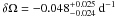
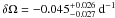
Figure 2 shows the marginal probability distribution for all relevant δΩ to have produced the data as derived from pairs with at least three common spots. The expectation value and the approximate 1σ confidence interval are δΩ = −0.048 ± 0.025 d-1. If we restrict the data to pairs with at least four common spots, we obtain the distribution shown in Fig. 3. The expectation value is δΩ = −0.045 ± 0.026 d-1. The width of the distribution is slightly broader because fewer pairs define the result. However, since these combinations fix the unknowns better because of the larger number of spots, the increase in width is marginal.
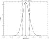 |
Fig. 2 Marginal distribution for the differential rotation parameter for a minimum of three spots. A total of 156 pairs were used. The average value is |
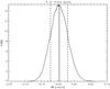 |
Fig. 3 Marginal distribution for the differential rotation parameter for a minimum of four spots. A total of 119 pairs were used. The average value is |
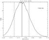 |
Fig. 4 Marginal distribution for the differential rotation parameter for a minimum of three spots in 1749 − 1761. A total of 55 pairs were used. The average value is |

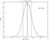 |
Fig. 5 Marginal distribution for the differential rotation parameter for a minimum of three spots in 1762 − 1799. A total of 101 pairs were used. The average value is |
The selection of pairs with five or more common spots delivers a very wide marginal distribution with an uncertainty of more than 0.05 in δΩ. The number of pairs used is then 86.
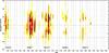 |
Fig. 6 Butterfly diagram from 1512 spot latitudes determined through the process of Bayesian inference of the differential rotation. Individual spots were broadened as if they had persisted for 80 days to obtain a smoother picture. |
The results are compatible with the differential rotation of the present Sun of δΩ = −0.0501 d-1 for a sin2-profile, according to Balthasar et al. (1986). The deviations of the expectation values based on Staudacher’s observations from that value are not significant. Both probability distributions in Figs. 2 and 3 show a slight tendency to a smaller differential rotation in 1749−1799 than today. This may be worth keeping in mind if more historical data are recovered, which would improve the statistics of the present work. Even if our study does not find a significantly different solar rotation profile, it is remarkable that these historical sunspot observations made by an amateur astronomer with a rather simple telescope reproduce the solar differential rotation nicely. The result is an indication for the quality of the drawings, which also led to the conclusion of an unusal butterfly diagram by Arlt (2009).
It may be worthwhile to check whether the average from the posterior distribution is a good measure of location for the differential rotation parameter. We find from simulated distributions of known differential rotation that the average is indeed very close to the true value if the posterior distribution becomes very small near the boundaries of the considered parameter interval. This is not necessary (and is in fact not true) for the individual distributions we obtained from individual pairs of drawings. The average of their average differential rotation parameters is not equal to the average obtained from the total posterior, and thus not close to the true value. All total posteriors shown in Figs. 2 − 5 are extremely small close to the interval boundaries of −0.5 and 0.5.
An interesting experiment is the splitting of the set of observations into two smaller sets. Figure 4 shows the marginal distribution for the drawings of 1749−1761, while Fig. 5 shows the distribution for 1762 − 1799. The differential rotation parameters are  and
and  , respectively, and indicate a decrease of the absolute value of the differential rotation during the second half of the 18th century. The difference is hardly significant though, because it is a 1σ-effect.
A large differential rotation bears the possibility of a hydrodynamic shear instability, as studied first by Watson (1981), who found the solar shear to be nearly marginal. A 3D study with viscosity by Arlt et al. (2005) led to higher limits for the differential rotation, while higher powers of sinb may alter these results (Dziembowski & Kosovichev 1987), which were not investigated here. If more data will become available and lead to a more accurate δΩ, a test on its hydrodynamic stability would be required.
A change of differential rotation could also be important because the butterfly diagram has a different appearance during cycles 0 and 1 (Arlt 2009). The equator was highly populated by spots and there is no clear migration direction of spot emergence. We can now use the spot latitudes determined as a side-product of the differential rotation determination and plot a butterfly diagram. Figure 6 shows the positions of the 1512 spots used in this analysis. Since we can only plot the positions of spots associated with each other in pairs of drawings, their number is much smaller than in Arlt (2009). The main features of that earlier paper are also visible in the present graph: relatively normal cycles 3 and 4, while cycles 0 and 1 show a highly populated equator, which persists also into cycle 2. The appearance of the first two cycles of Staudacher’s period somewhat resembles a topology that dynamo theorists call symmetric solutions of the magnetic field, in contrast to the anti-symmetric situation that we observe today. Symmetry here is meant with respect to the equator. Of course we do not have magnetic field polarities at hand for historical observations, and consequently the true topology of the dynamo mode will hardly ever be accessible.
Mean-field models typically show that symmetric and anti-symmetric solutions have very similar excitation thresholds (e.g. Chatterjee et al. 2004; Dikpati et al. 2004; Bonanno et al. 2005) and it is not straightforward to assume the one should dominate the other all the time. A small change in δΩ might have favoured the symmetric solution in the 18th century, which exhibited a different butterfly diagram. Mean-field dynamo models with a back-reaction on the differential rotation tend to show excursions to symmetric geometry for reduced differential rotation though (e.g. Tobias 1997; Küker et al. 1999; Bushby 2006). Before we speculate too much, we conclude here that there is an indication for a change of δΩ during the 18th century, and we aim to stimulate future studies on the possible competition of the individual dynamo modes.
Acknowledgments
R.A. is grateful to the Deutsche Forschungsgemeinschaft for supporting this work within the grant Ar355/6-1 and for the hospitality of the Kiepenheuer Institute for Solar Physics where the work has been initiated during a one-month visit.
References
- Arlt, R. 2008, Sol. Phys., 247, 399 [NASA ADS] [CrossRef] [Google Scholar]
- Arlt, R. 2009, Sol. Phys., 255, 143 [NASA ADS] [CrossRef] [Google Scholar]
- Arlt, R., Sule, A., & Rüdiger, G. 2005, A&A, 441, 1171 [NASA ADS] [CrossRef] [EDP Sciences] [Google Scholar]
- Balthasar, H., Vázquez, M., & Wöhl, H. 1986, A&A, 155, 87 [NASA ADS] [Google Scholar]
- Benevolenskaya, E. E., Hoeksema, J. T., Kosovichev, A. G., & Scherrer, P. H. 1999, ApJ, 517, L163 [NASA ADS] [CrossRef] [Google Scholar]
- Bonanno, A., Elstner, D., Belvedere, G., & Rüdiger, G. 2005, Astron. Nachr., 326, 170 [NASA ADS] [CrossRef] [Google Scholar]
- Bushby, P. J. 2006, MNRAS, 371, 772 [Google Scholar]
- Chatterjee, P., Nandy, D., & Choudhuri, A. R. 2004, A&A, 427, 1019 [NASA ADS] [CrossRef] [EDP Sciences] [Google Scholar]
- Dikpati, M., de Toma, G., & Gilman, P. A. 2004, ApJ, 601, 1136 [NASA ADS] [CrossRef] [Google Scholar]
- Dziembowski, W., & Kosovichev, A. 1987, Acta Astron., 37, 341 [NASA ADS] [Google Scholar]
- Frasca, A., Fröhlich, H.-E., Bonanno, A., et al. 2011, A&A, 532, A81 [NASA ADS] [CrossRef] [EDP Sciences] [Google Scholar]
- Fröhlich, H.-E., Küker, M., Hatzes, A. P., & Strassmeier, K. G. 2009, A&A, 506, 263 [NASA ADS] [CrossRef] [EDP Sciences] [Google Scholar]
- Komm, R., Howe, R., Durney, B. R., & Hill, F. 2003, ApJ, 586, 650 [NASA ADS] [CrossRef] [Google Scholar]
- Korzennik, S. G., & Eff-Darwich, A. 2011, J. Phys. Conf. Ser., 271, 012067 [NASA ADS] [CrossRef] [Google Scholar]
- Küker, M., Arlt, R., & Rüdiger, G. 1999, A&A, 343, 977 [NASA ADS] [Google Scholar]
- Malkus, W. V. R., & Proctor, M. R. E. 1975, JFM, 67, 417 [Google Scholar]
- Pizzo, V., Schwenn, R., Marsch, E., et al. 1983, ApJ, 271, 335 [NASA ADS] [CrossRef] [Google Scholar]
- Press, W. H., Teukolsky, S. A., Vetterling, W. T., & Flannery, B. P. 2007, Numerical Recipes, 3rd edn. (Cambridge: Cambridge Univ. Press) [Google Scholar]
- Ribes, J., & Nesme-Ribes, E. 1993, A&A, 276, 549 [NASA ADS] [Google Scholar]
- Tobias, S. M. 1997, A&A, 322, 1007 [NASA ADS] [Google Scholar]
- Wall, M. E., Rechtsteiner, A., & Rocha, L. M. 2003, in A practical approach to microarray data analysis, ed. D. P. Berrar, W. Dubitzky, & M. Granzow (Norwell: Kluwer) [Google Scholar]
- Watson, M. 1981, Geophys. Astrophys. Fluid Dyn., 16, 285 [Google Scholar]
All Tables
Comparison of the number of measurements versus the number of free parameters for given spot numbers and different methods using pairs of drawings.
All Figures
|
Fig. 1 Association of spots in the two superimposed images of 1761 June 23 (spots coloured in green) and 1761 June 24 (spots coloured in red). The difference in position angles determined by rotational matching is 29.8°. |
| In the text | |
|
Fig. 2 Marginal distribution for the differential rotation parameter for a minimum of three spots. A total of 156 pairs were used. The average value is |
| In the text | |
|
Fig. 3 Marginal distribution for the differential rotation parameter for a minimum of four spots. A total of 119 pairs were used. The average value is |
| In the text | |
|
Fig. 4 Marginal distribution for the differential rotation parameter for a minimum of three spots in 1749 − 1761. A total of 55 pairs were used. The average value is |
| In the text | |
|
Fig. 5 Marginal distribution for the differential rotation parameter for a minimum of three spots in 1762 − 1799. A total of 101 pairs were used. The average value is |
| In the text | |
|
Fig. 6 Butterfly diagram from 1512 spot latitudes determined through the process of Bayesian inference of the differential rotation. Individual spots were broadened as if they had persisted for 80 days to obtain a smoother picture. |
| In the text | |
Current usage metrics show cumulative count of Article Views (full-text article views including HTML views, PDF and ePub downloads, according to the available data) and Abstracts Views on Vision4Press platform.
Data correspond to usage on the plateform after 2015. The current usage metrics is available 48-96 hours after online publication and is updated daily on week days.
Initial download of the metrics may take a while.