| Issue |
A&A
Volume 543, July 2012
|
|
|---|---|---|
| Article Number | A139 | |
| Number of page(s) | 10 | |
| Section | Atomic, molecular, and nuclear data | |
| DOI | https://doi.org/10.1051/0004-6361/201219023 | |
| Published online | 12 July 2012 | |
Atomic data for astrophysics: Fe xii soft X-ray lines⋆
1 DAMTP, Centre for Mathematical Sciences, Wilberforce Road, Cambridge, CB3 0WA, UK
e-mail: This email address is being protected from spambots. You need JavaScript enabled to view it.
2 Department of Physics and Astronomy, University College London, Gower Street, London, WC1E 6BT, UK
3 Department of Physics, University of Strathclyde, Glasgow, G4 0NG, UK
Received: 12 February 2012
Accepted: 30 May 2012
Abstract
We present new large-scale R-matrix (up to n = 4) and distorted-wave (DW, up to n = 6) scattering calculations for electron collisional excitation of Fe xii. The first aim is to provide accurate atomic data for the soft X-rays, where strong decays from the n = 4 levels are present. As found in previous work on Fe x, resonances attached to n = 4 levels increase the cross-sections for excitations from the ground state to some n = 4 levels, when compared to DW calculations. Cascading from higher levels is also important. We provide a number of models and line intensities, and list a number of strong unidentified lines. The second aim is to assess the effects of the large R-matrix calculation on the n = 3 transitions. Compared to our previous (n = 3) R-matrix calculation, we find overall excellent agreement to within a few percent, however a few key density diagnostic EUV intensities differ by about 60% at coronal densities. The new atomic data result in lower electron densities, resolving previous discrepancies with solar observations.
Key words: atomic data / line: identification / techniques: spectroscopic / Sun: corona
The full dataset (energies, transition probabilities and rates) are available in electronic form at our APAP website (http://www.apap-network.org) as well as at the CDS via anonymous ftp to cdsarc.u-strasbg.fr (130.79.128.5) or via http://cdsarc.u-strasbg.fr/viz-bin/qcat?J/A+A/543/A139
© ESO, 2012
1. Introduction
The soft X-ray (50–170 Å) spectrum of the quiet and active Sun is rich in n = 4 → n = 3 transitions from highly ionised iron ions, from Fe vii to Fe xvi (see, e.g. Fawcett et al. 1968; Manson 1972; Behring et al. 1972). Very little atomic data are currently available for these ions and the majority of the spectral lines still await firm identification, despite the fact that various current missions are routinely observing the soft X-rays. The Solar Dynamic Observatory (SDO) Atmospheric Imaging Assembly (AIA, see Lemen et al. 2012) and the Extreme ultraviolet Variability Experiment (EVE) (Woods et al. 2012) have been observing the Sun in the soft X-rays. Soft X-ray spectra of stellar coronae are also routinely observed with the Chandra Low Energy Transmission Grating spectrometer (LETG, see Brinkman et al. 2000).
The atomic data for Fe viii and Fe ix relevant for the soft X-rays have recently been discussed in O’Dwyer et al. (2012), where new distorted wave (DW) scattering calculations for these two ions were presented. The main issues related to calculating accurate atomic data for the n = 4 levels are discussed in Del Zanna et al. (2012), where new atomic data for Fe x have been presented.
Here, we present new large-scale scattering calculations for the Fe xii soft X-ray lines. We also review the extreme-ultraviolet (EUV) lines, given their importance for many current missions, especially for the Hinode EUV Imaging Spectrometer (EIS, see Culhane et al. 2007) where Fe xii lines are prominent in its two spectral ranges (SW: 166–212 Å; LW: 245–291 Å). Fe xii lines are routinely used to measure electron densities, in particular the ratio of the two self-blends at 186.88 and 195.12 Å. These strong lines provide the best density diagnostic for the quiet solar corona for this ion. It has been pointed out by many authors (see, e.g. Young et al. 2009) that these diagnostics produce higher densities than those obtained with other ions formed close in temperature. A full benchmark of the coronal density diagnostics available to Hinode EIS was performed by Del Zanna (2012), where these inconsistencies, although not very large, were confirmed. We therefore aim to investigate whether a larger calculation can resolve these discrepancies.
This paper is organised as follows. In Sect. 2, we give a brief review of previous observations and atomic calculations. In Sect. 3 we outline the methods adopted for the scattering calculations. In Sect. 4 we present our results and in Sect. 5 we reach our conclusions.
2. Previous observations and atomic data for Fe xii
A history of the identifications of all the EUV and visible forbidden lines (from within the n = 3 configurations) for Fe xii was given in detail in Del Zanna & Mason (2005) and is not repeated here. Historically, large discrepancies between observed and predicted intensities of EUV transitions from the n = 3 levels were found to be present. These discrepancies were finally resolved by Storey et al. (2005) via an R-matrix electron collisional calculation carried-out within the Iron Project. References to earlier calculations for the n = 3 levels are given in Storey et al. (2005).
The configuration basis describing the target adopted by Storey et al. (2005) included 12 of the main n = 3 configurations. For the scattering calculation the lowest 58 LS terms were included, giving rise to 143 fine-structure levels. The expansion of each scattered electron partial wave was over a basis of 20 functions within the R-matrix boundary, and the partial wave expansion extended to a maximum total orbital angular momentum quantum number of L = 18. The outer region calculation was carried out using the intermediate-coupling frame transformation method (ICFT) described by Griffin et al. (1998), up to a total angular momentum quantum number J = 15. The non-exchange calculation extended from J = 16 to J = 50.
Del Zanna & Mason (2005) complemented the Storey et al. (2005) collisional rates with a set of A-values. We refer to this ion model here as DM05. Del Zanna & Mason (2005) benchmarked line intensities against various experimental data. Excellent agreement was found, and a large number of new identifications were proposed. These new observed energies are adopted here. These data have been used since 2005 within the CHIANTI database (Dere et al. 1997; Landi et al. 2006). Later, Del Zanna (2012) used Hinode EIS observations to confirm most of the new identifications.
For the soft X-rays (n = 4 → n = 3 transitions), the identifications of some of the 3s23p2 4l (l = s, p, d, f) levels are due to the fundamental laboratory work by Fawcett et al. (1972). It is important to keep in mind that only lines with strong oscillator strengths were identified, that some identifications were tentative, and that a large number of lines in the spectra were left unidentified. We have re-analysed some of Fawcett’s plates as part of a larger project to sort out the identifications in the Fe soft X-ray spectrum.
3. Methods
The atomic structure calculations were carried out using the autostructure program (Badnell 1997) which constructs target wavefunctions using radial wavefunctions calculated in a scaled Thomas-Fermi-Dirac statistical model potential with a set of scaling parameters. The Breit-Pauli distorted wave calculations were carried out using the recent development of the autostructure code, described in detail in Badnell (2011). Collision strengths are calculated at the same set of final scattered energies for all transitions. “Top-up” for the contribution of high partial waves is done using the same Breit-Pauli methods and subroutines implemented in the R-matrix outer-region code STGF. The program also provides radiative rates and infinite energy Born limits. These limits are particularly important for two aspects. First, they allow a consistency check of the collision strengths in the scaled Burgess & Tully (1992) domain (see also Burgess et al. 1997). Second, they are used in the interpolation of the collision strengths at high energies when calculating the Maxwellian averages.
The R-matrix method used in the inner region of the scattering calculation is described in Hummer et al. (1993) and Berrington et al. (1995). We performed it in LS coupling and included the mass-velocity and Darwin relativistic operators. The outer region calculation used the ICFT method (Griffin et al. 1998). Dipole-allowed transitions were topped-up to infinite partial wave using an intermediate coupling version of the Coulomb-Bethe method as described by Burgess (1974) while non-dipole allowed transitions were topped-up assuming that the collision strengths form a geometric progression in J (see Badnell & Griffin 2001). The collision strengths were extended to high energies by interpolation using the appropriate high-energy limits in the Burgess & Tully (1992) scaled domain. The high-energy limits were calculated with autostructure for both optically-allowed (see Burgess et al. 1997) and non-dipole allowed transitions (see Chidichimo et al. 2003). The temperature-dependent effective collisions strength Υ(i − j) were calculated by assuming a Maxwellian electron distribution and linear integration with the final energy of the colliding electron.
4. Results
Several calculations have been performed with different size target expansions and corresponding ion population models have been constructed to predict line intensities and compare with observations. A summary of our investigations is presented here.
We started with various DW calculations systematically increasing the number of configurations up to and including those with n = 6 valence orbitals. The DW rates for the higher levels were supplemented with the Storey et al. (2005) R-matrix data, to ensure that the metastable levels are correctly populated.
We then performed separate structure calculations for each ion model to calculate all of the radiative data for all transitions among the levels. This ensures that all the cascading from the target configurations is included. We then calculated the level populations and the relative line intensities so as to find out which lines are expected to be strongest. We then compared the results to the laboratory plates of Fawcett and to solar spectra.
As in the Fe x case (Del Zanna et al. 2012), we found large discrepancies between observed and predicted intensities, in particular for the decays from the 3s23p2 4s levels. Exactly as in the Fe x case, we also predicted some (unidentified) decays from the 3s 3p3 4s levels to be even stronger, in coronal conditions, than the decays from the 3s23p2 4s levels (as we will show below).
We followed the procedure outlined in the Fe x case to estimate which configurations would be likely to be producing resonances in the collision strengths for the spectroscopically important configurations/levels. For Fe x, we found that the excitations to the 3s2 3p4 4s levels are significantly underestimated by the DW calculations, mostly because of resonances due to the 3s2 3p4 4p levels. Similarly, we also found the 3s23p2 4s levels in Fe xii to be affected by the same issues. We found that most resonance excitations to the n = 4 levels come from a number of configurations which we have then included in the scattering calculation.
4.1. The R-matrix and DW calculations for the n = 3, 4 levels
As our configuration basis set we have chosen the complete set of 36 configurations shown in Fig. 1 and listed in Table 1. The scaling parameters λnl for the potentials in which the orbital functions are calculated are also given in Table 1. A full R-matrix calculation with all the n = 4 levels is prohibitive at present, because it would involve 1538 LS terms and 4071 levels. For the scattering close-coupling calculation, we retained 912 fine-structure levels arising from the first 356 LS terms of the lowest set of 20 configurations (see Fig. 1). We have performed both an ICFT R-matrix and a DW calculation using the same basis. They have both been challenging large-scale calculations.
Table 2 presents a selection of fine-structure target level energies Et, compared to experimental energies Eexp. The latter have been obtained from Del Zanna & Mason (2005) for the n = 3 levels, otherwise from a selection of Fawcett et al. (1972) identifications which we assessed individually.
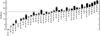 |
Fig. 1 Term energies of the target levels (36 configurations) for the n = 4 calculations. The 356 terms which produce levels having energies below the dashed line have been retained for the close-coupling expansion. |
Target electron configuration basis and orbital scaling parameters λnl for the R-matrix and DW runs.
There is good overall agreement in terms of energy differences between levels. A set of “best” energies Eb was obtained with a quadratic fit between the Eexp and Et values. The Eb values were used (together with the Eexp ones) within the R-matrix calculation to obtain an accurate position of the resonance thresholds. They were also used to calculate the transition probabilities, which were computed separately using the full n = 4 target basis. We then built two ion population models, using these transition probabilities, one with the R-matrix rates (hereafter RM4) and one with just the DW rates (hereafter DW4).
Level energies for Fe xii (n = 3,4).
The expansion of each scattered electron partial wave was carried out over a basis of 19 functions within the R-matrix boundary and the partial wave expansion extended to a maximum total orbital angular momentum quantum number of L = 16. This produces accurate collision strengths up to about 80 Ryd.
The outer region calculation includes exchange up to a total angular momentum quantum number J = 26/2. We have supplemented the exchange contributions with a non-exchange calculation extending from J = 28/2 to J = 74/2. The outer region exchange calculation was performed in a number of stages. A coarse energy mesh was chosen above all resonances. The resonance region itself was calculated with an increasing number of energies to check for convergence, as was done for the Iron Project Fe xi calculation (Del Zanna et al. 2010). The results presented here are obtained with 8800 points in the resonance region.
We then compared the collision strengths and their thermal averages with the DW results and those by Storey et al. (2005) for the n = 3 levels. The comparisons for a selection of levels giving rise to important transitions are displayed in Figs. 2–7. Excellent agreement between the background R-matrix and the DW collision strengths is found in all cases. This is to be expected since they both use the same target. Excellent agreement is found with the Storey et al. (2005) data for all the dipole-allowed transitions (e.g. Fig. 7). However, significant increases are found for a number of forbidden transitions. We will return to this issue below.
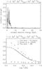 |
Fig. 2 Above: collision strength for the 1–2 line, averaged over 0.1 Ryd in the resonance region. The data points are displayed in histogram mode. Boxes indicate the DW values. Below: thermally-averaged collision strengths, compared to the R-matrix results of Storey et al. (2005) and the DW ones. |
 |
Fig. 8 Same as Fig. 2, for the 1–288 transition, the strongest soft X-ray line among those identified by Fawcett et al. (1972). Note the strong enhancement due to the resonances. |
We then looked at the transitions to the n = 4 levels. Again, good agreement between the R-matrix background and the DW data is found. However, as we expected, we find significant resonance contribution for transitions to a number of levels, in particular to the 3s2 3p2 4s ones. Figure 8 shows the collision strengths for the 79.5 Å transition as an example. The enhancements are not as strong as we found in the Fe x case, but become increasingly important at low temperatures.
4.2. The n = 3 main EUV density diagnostics
The relative intensities of the brightest lines from the n = 3 levels at coronal densities are shown in Table 3. We show both the values obtained from the present RM4 model and from the previous DM05, based on the Storey et al. (2005) collision rates. For most cases, we obtain the same intensities with these two models. However, for the important density diagnostic lines we find significantly increased line intensities. In particular, the self-blend of the 3–39 and 2–36 transitions at 186.88 Å (identified in Del Zanna & Mason 2005) and the 3–34 one at 196.64 Å are increased by 60%. These two lines are the best electron density diagnostics in the EUV for this ion, and are prominent in Hinode EIS spectra. We found no significant differences at densities towards the high-density limits for these transitions.
Relative intensities of the brightest lines in Fe xii in the EUV and the visible.
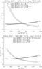 |
Fig. 9 Emissivity ratio curves relative to the main Fe xii EUV transitions observed by Hinode EIS on 2007 Aug. 19, using the DM05 atomic model (above) and the present RM4+DW6 (below). The wavelengths and indices of the transitions are given, as well as the observed intensity Iob (see Del Zanna 2012, for details). |
The main consequence of the present model is to lower the densities obtained from these diagnostics. This is what was needed to remove the discrepancy with the densities obtained from other ions. We have analysed various observations at low and high densities and found excellent agreement using the present atomic data. One example is provided in Fig. 9. We have considered the Hinode EIS off-limb active region spectra recorded on 2007 Aug. 19, and used in Del Zanna (2012) to benchmark all the coronal ions. As seen in other cases, Fe xii produced higher densities compared to those from all the other ions. Figure 9 (top) shows the emissivity ratio curves obtained with the previous DM05 atomic data, indicating a density log Ne [cm-3] = 8.8. These curves are obtained by dividing the observed intensities of the lines with their predicted emissivity as a function of the electron density. The crossing of the curves indicates agreement between observed and predicted line intensities at log Ne [cm-3] = 8.8 (for further details on this emissivity ratio technique see Del Zanna et al. 2004). The measurements from other ions emitted at similar temperatures such as Si x indicated a density log Ne [cm-3] = 8.5. Figure 9 (bottom) shows the emissivity ratio curves obtained with the current RM4+DW6 model (an extension of RM4, as discussed below), indicating a density log Ne [cm-3] = 8.5, in excellent agreement with the Si x results.
 |
Fig. 10 Collision strengths from the RM4 calculation for a selection of transitions, averaged over 0.5 Ryd in the resonance region (displayed in histogram mode, thin black lines). The thick (blue) lines indicate the Storey et al. (2005) values, and the thicker (grey) lines those from the RM4_58T calculation. |
Populations of a few Fe xii (n = 3) key levels.
One question then naturally arises: what causes these higher intensities at low coronal densities? The differences with the previous DM05 model turn out to be due to a combination of subtle effects, mostly due to small increases in the excitations of various levels due to the extra resonances we obtain with this much larger scattering calculation.
In order to make sure that no other effects are in play, we performed a full new R-matrix calculation where we adopted the same target basis and orbital scaling parameters as in RM4, but included this time only the lowest 58 terms and 143 levels as was done in Storey et al. (2005). In order to match the energy resolution of the RM4 calculation, we calculated collision strengths for 4200 points in the resonance region. We refer to this 58-terms calculation as RM4_58T. Figure 10 shows a comparison between the collision strengths of a few key transitions for the RM4, the RM4_58T, and the Storey et al. (2005) R-matrix calculations. Overall agreement between the RM4_58T and the Storey et al. (2005) results is found for all transitions, however the RM4 present some clear enhancements. Table 4 provides a summary of the populations of some of the key levels, as calculated with the previous (DM05) and current (RM4) ion models at quiet-Sun densities (log Ne [cm-3] = 8).
Relative intensities of the brightest Fe xii lines in in the soft X-rays.
The increase in the intensity of the 3–39 186.88 Å transition is due to an increased population for level 39, which in turn is mainly due to two effects, the excitation from level 3 (by 87%) and that one from the ground state (8%). The first is enhanced due to an increased population of level 3 from 4.7% to 7.2% (i.e. by 50%). In turn, level 3 becomes populated directly from the ground state by 18% and by 80% via cascading from a range of n = 3 levels. The direct excitation from the ground state is increased as shown in Fig. 10. Cascading for level 3 is also increased because of increases in the populations of the upper levels (e.g. levels 10), due to the extra resonances in our RM4 model (see Fig. 10). The second excitation for level 39 (from the ground state) is also increased as shown in Fig. 10.
Similar effects occur for the other density diagnostic, the 3–34 196.65 Å line, as shown in Table 4 and Fig. 10. Level 34 is mainly populated via excitation from level 3 (by 83%) and from the ground state (10%), and both excitations are enhanced in the present model.
4.3. The soft X-ray lines
To look at the effects of resonances, we have built two ion models for the n = 4 levels. One with the R-matrix n = 4 rates (RM4), and one with the DW rates (DW4). In both cases, the same set of A-values (obtained with experimental and best energies) were used. The relative intensities of the brightest Fe xii soft X-rays lines are shown in Table 5. The lines that turn out to be most affected by resonance enhancement are those within the 3s2 3p2 4s and 3s2 3p2 4d configurations, where increases of about 50% are found, i.e. not as much as we found for the Fe x case, but still significant.
We looked at the populations of some 3s2 3p2 4l levels, and found that the 3s2 3p2 4s are affected by about 30% by cascading from higher levels, while for the others the main excitation is directly from the ground state.
As in the Fe x case, both the DW and R-matrix calculations indicate that a number of strong transitions are unidentified, in particular those from the 3s 3p3 4s and 3s2 3p2 4p levels. Indeed, at coronal densities, many of the strongest transitions are unidentified.
Main cascading affecting the populations of two Fe xii (n = 4) levels.
4.4. DW calculations for the n = 5, 6 levels and cascading effects
To estimate the effects of further cascading from even higher levels, we built a new target by adding the following configurations to the R-matrix n = 4 one (RM4): 3s2 3p2 5l (l = s, p, d, f, g), 3s 3p3 5l (l = s, p, d, f, g), 3p4 5l (l = s, p, d, f, g), 3s2 3p2 6l (l = s, p, d, f, g), 3s 3p3 6l (l = s, p, d, f, g), 3p4 6l (l = s, p, d, f, g). We kept the scaling parameters for the n = 4 the same, and obtained those for the n = 5,6, which are listed in Table 1. This was done to try and keep similar energies (and ordering of the levels) for the n = 4 levels. The total target is very large. It comprises 66 configurations, 1970 LS terms and 5143 fine-structure levels. We then used the DW code to calculate the excitation rates up to all of these levels, but just from the lowest 41 arising from the 3s2 3p3, 3s 3p4, and 3s2 3p2 3d configurations. This enables us to treat all possible metastable levels populating the upper ones.
We then calculated separately the radiative rates between all the 5143 levels, and matched the ordering of this calculation with that of the 912-levels RM4. We then merged the rates and A-values from RM4 with those from this DW run, and built an ion model, which we indicate as RM4+DW6. The relative intensities with the RM4+DW6 model of the main soft X-ray lines are shown in Table 5 while those for the EUV lines are listed in Table 3.
Some transitions from the 3s2 3p2 4s and 3s2 3p2 4p configurations are increased by about 10%. The decays from the 3s2 3p2 4d levels are increased by up to about 30%. Some increases for the 3d transitions due to cascading effects are also present, but are normally smaller, of the order of 5%.
One interesting issue is whether the RM4+DW6 model includes all the main cascading processes for the n = 4 levels, and how much the contribution of further cascading from n ≥ 7 levels would be. In our case, we expect further cascading from levels with n ≥ 7 to be small, of the order of a few percent at most. The cascading obviously becomes smaller with increasing principal quantum number n since the direct excitations from the ground state (hence the populations) decrease as n-3. However, an exact calculation is non-trivial, requiring a proper scattering and structure calculation, and the building of a very large ion model. Such a calculation is left to a future paper, considering that the corrections would be of the same order (or smaller) as those arising from the resonance enhancements due to the n ≥ 5 levels, not included in the R-matrix calculation.
For Fe x, Malinovsky et al. (1980) performed some approximate calculations to estimate the contributions by cascading to the 3s2 3p4 4s levels. They assumed that the main cascading to the 3s2 3p4 4s levels would come from the 3s2 3p4np levels. They then estimated approximate values for the excitation from the ground state assuming that they vary as (n − μnL)-3, where μnL is the quantum defect of the nL orbital. They also assumed that the branching ratios to be constant and equal to the values for n = 5. They found that cascading from the 3s2 3p4 5p increased the intensities of the 3s2 3p4 4s levels by at most 16%. Cascading from the 3s2 3p4np (n ≥ 6) added at most a further 10%.
We now look at two of the transitions most affected (see Table 5) by cascading in Fe xii, and show how complex cascading actually is. We consider three ion models, the RM4 and RM4+DW6, and an intermediate (RM4+DW5) where we have only retained the n ≤ 5 levels. Details are given in Table 6.
We consider first the 1–288 79.488 Å transition, the main decay from the 3s2 3p2 4s 4P5/2 level. We find that adding n = 5 levels increases the population by 7%, while adding the n = 6 ones adds only a further 2.6% overall. Looking in detail at which levels contribute most, we find that by far the dominant cascading comes from a 3s 3p3 4s 4S3/2 level (17%), and not from the 3s2 3p2np ones as one would have expected. This occurs because the 3s 3p3 4s 4S3/2 level has a strong forbidden excitation rate from the ground state (0.45 at 1.26 MK) and a strong allowed decay (A = 3 × 10¹⁰ s-1) to the 3s2 3p2 4s 4P5/2 (288) level, with a branching ratio of 0.3. The next level of the Rydberg series (3s 3p3 5s 4S3/2) has negligible contribution, having a small excitation rate (0.007 at 1.26 MK) from the ground state and a small branching ratio (0.0002) to level 288. The 3s2 3p2np 4S3/2 levels contribute 7.0, 5.7, and 2.0% respectively, however their excitation rates from the ground state (0.4, 0.08, 0.04 at 1.26 MK) and branching ratios (0.02, 0.12, 0.07) do not have a simple behavior. Further smaller contributions come from the 3s2 3p2np 4D7/2 levels.
The situation is quite different for the higher 3s2 3p2 4d 4F5/2 (487) level. The n = 4 levels produce negligible cascading on its population. Adding n = 5 levels increases significantly (29%) its population. The n = 6 levels, on the other hand, do not produce any significant cascading effects. The main cascading (9.6%) comes from a 3s2 3p2 5p 4P3/2 level. Cascading from the 3s2 3p2 6p 4P3/2 is negligible ( ≤ 0.01%). Further cascading comes from the 3s2 3p2 5f 4D7/2 and a large number of other n = 5 levels.
5. Summary and conclusions
We have presented the first R-matrix calculations for the n = 4 levels in Fe xii. We have found the same issues we discovered in Fe x. Given their small collision strengths for excitations from the ground, the 3s2 3p2 4s levels are mainly affected in two ways. First, the rates are increased significantly by resonances which are attached mainly to the 3s2 3p2 4p levels. Second, the population of these levels is enhanced by cascading from higher levels. These two effects are not as large as in Fe x, but are nevertheless significant.
We found that a large number of strong transitions are unidentified, as we saw in other ions, in particular the decays from the 3s 3p3 4s levels. The identifications of these levels will be discussed in a separate paper.
The somewhat surprising result of these new calculations is the enhancement in the populations of some important levels producing the best electron density diagnostics in the EUV for this ion. We find previous discrepancies to be resolved. The reasons for the enhancements are subtle and show how difficult it is to obtain a correct atomic model for complex ions such as Fe xii.
Acknowledgments
G.D.Z. acknowledges the support from STFC via the Advanced Fellowship programme. We acknowledge support from STFC for the UK APAP network. B. C. Fawcett is thanked for his contribution in rescuing some of his original plates, and for the continuous encouragement over the years.
References
- Badnell, N. R. 1997, J. Phys. B At. Mol. Phys., 30, 1 [NASA ADS] [CrossRef] [Google Scholar]
- Badnell, N. R. 2011, Comput. Phys. Commun., 182, 1528 [NASA ADS] [CrossRef] [Google Scholar]
- Badnell, N. R., & Griffin, D. C. 2001, J. Phys. B At. Mol. Phys., 34, 681 [NASA ADS] [CrossRef] [Google Scholar]
- Behring, W. E., Cohen, L., Doschek, G. A., & Feldman, U. 1972, ApJ, 175, 493 [NASA ADS] [CrossRef] [Google Scholar]
- Berrington, K. A., Eissner, W. B., & Norrington, P. H. 1995, Comput. Phys. Commun., 92, 290 [NASA ADS] [CrossRef] [Google Scholar]
- Brinkman, A. C., Gunsing, C. J. T., Kaastra, J. S., et al. 2000, ApJ, 530, L111 [NASA ADS] [CrossRef] [Google Scholar]
- Burgess, A. 1974, J. Phys. B At. Mol. Phys., 7, L364 [NASA ADS] [CrossRef] [Google Scholar]
- Burgess, A., & Tully, J. A. 1992, A&A, 254, 436 [NASA ADS] [Google Scholar]
- Burgess, A., Chidichimo, M. C., & Tully, J. A. 1997, J. Phys. B At. Mol. Phys., 30, 33 [NASA ADS] [CrossRef] [Google Scholar]
- Chidichimo, M. C., Badnell, N. R., & Tully, J. A. 2003, A&A, 401, 1177 [NASA ADS] [CrossRef] [EDP Sciences] [Google Scholar]
- Culhane, J. L., Harra, L. K., James, A. M., et al. 2007, Sol. Phys., 243, 19 [Google Scholar]
- Del Zanna, G. 2012, A&A, 537, A38 [NASA ADS] [CrossRef] [EDP Sciences] [Google Scholar]
- Del Zanna, G., & Mason, H. E. 2005, A&A, 433, 731 [NASA ADS] [CrossRef] [EDP Sciences] [Google Scholar]
- Del Zanna, G., Berrington, K. A., & Mason, H. E. 2004, A&A, 422, 731 [NASA ADS] [CrossRef] [EDP Sciences] [Google Scholar]
- Del Zanna, G., Storey, P. J., & Mason, H. E. 2010, A&A, 514, A40 [NASA ADS] [CrossRef] [EDP Sciences] [Google Scholar]
- Del Zanna, G., Storey, P. J., Badnell, N. R., & Mason, H. E. 2012, A&A, 541, A90 [NASA ADS] [CrossRef] [EDP Sciences] [Google Scholar]
- Dere, K. P., Landi, E., Mason, H. E., Monsignori Fossi, B. C., & Young, P. R. 1997, A&AS, 125, 149 [NASA ADS] [CrossRef] [EDP Sciences] [Google Scholar]
- Fawcett, B. C., Peacock, N. J., & Cowan, R. D. 1968, J. Phys. B At. Mol. Phys., 1, 295 [NASA ADS] [CrossRef] [Google Scholar]
- Fawcett, B. C., Kononov, E. Y., Hayes, R. W., & Cowan, R. D. 1972, J. Phys. B At. Mol. Phys., 5, 1255 [Google Scholar]
- Griffin, D. C., Badnell, N. R., & Pindzola, M. S. 1998, J. Phys. B At. Mol. Phys., 31, 3713 [NASA ADS] [CrossRef] [Google Scholar]
- Hummer, D. G., Berrington, K. A., Eissner, W., et al. 1993, A&A, 279, 298 [NASA ADS] [Google Scholar]
- Landi, E., Del Zanna, G., Young, P. R., et al. 2006, ApJS, 162, 261 [NASA ADS] [CrossRef] [Google Scholar]
- Lemen, J. R., Title, A. M., Akin, D. J., et al. 2012, Sol. Phys., 275, 17 [NASA ADS] [CrossRef] [Google Scholar]
- Malinovsky, M., Dubau, J., & Sahal-Brechot, S. 1980, ApJ, 235, 665 [NASA ADS] [CrossRef] [Google Scholar]
- Manson, J. E. 1972, Sol. Phys., 27, 107 [NASA ADS] [CrossRef] [Google Scholar]
- O’Dwyer, B., Del Zanna, G., Badnell, N. R., Mason, H. E., & Storey, P. J. 2012, A&A, 537, A22 [NASA ADS] [CrossRef] [EDP Sciences] [Google Scholar]
- Storey, P. J., Del Zanna, G., Mason, H. E., & Zeippen, C. 2005, A&A, 433, 717 [NASA ADS] [CrossRef] [EDP Sciences] [Google Scholar]
- Woods, T. N., Eparvier, F. G., Hock, R., et al. 2012, Sol. Phys., 275, 115 [Google Scholar]
- Young, P. R., Watanabe, T., Hara, H., & Mariska, J. T. 2009, A&A, 495, 587 [NASA ADS] [CrossRef] [EDP Sciences] [Google Scholar]
All Tables
Target electron configuration basis and orbital scaling parameters λnl for the R-matrix and DW runs.
Relative intensities of the brightest lines in Fe xii in the EUV and the visible.
All Figures
|
Fig. 1 Term energies of the target levels (36 configurations) for the n = 4 calculations. The 356 terms which produce levels having energies below the dashed line have been retained for the close-coupling expansion. |
| In the text | |
|
Fig. 2 Above: collision strength for the 1–2 line, averaged over 0.1 Ryd in the resonance region. The data points are displayed in histogram mode. Boxes indicate the DW values. Below: thermally-averaged collision strengths, compared to the R-matrix results of Storey et al. (2005) and the DW ones. |
| In the text | |
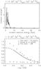 |
Fig. 3 Same as Fig. 2, for the 1–3 transition. |
| In the text | |
 |
Fig. 4 Same as Fig. 2, for the 1–10 transition. |
| In the text | |
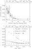 |
Fig. 5 Same as Fig. 2, for the 1–34 transition. |
| In the text | |
 |
Fig. 6 Same as Fig. 2, for the 1–39 transition. |
| In the text | |
 |
Fig. 7 Same as Fig. 2, for the 3–39 transition. |
| In the text | |
|
Fig. 8 Same as Fig. 2, for the 1–288 transition, the strongest soft X-ray line among those identified by Fawcett et al. (1972). Note the strong enhancement due to the resonances. |
| In the text | |
|
Fig. 9 Emissivity ratio curves relative to the main Fe xii EUV transitions observed by Hinode EIS on 2007 Aug. 19, using the DM05 atomic model (above) and the present RM4+DW6 (below). The wavelengths and indices of the transitions are given, as well as the observed intensity Iob (see Del Zanna 2012, for details). |
| In the text | |
|
Fig. 10 Collision strengths from the RM4 calculation for a selection of transitions, averaged over 0.5 Ryd in the resonance region (displayed in histogram mode, thin black lines). The thick (blue) lines indicate the Storey et al. (2005) values, and the thicker (grey) lines those from the RM4_58T calculation. |
| In the text | |
Current usage metrics show cumulative count of Article Views (full-text article views including HTML views, PDF and ePub downloads, according to the available data) and Abstracts Views on Vision4Press platform.
Data correspond to usage on the plateform after 2015. The current usage metrics is available 48-96 hours after online publication and is updated daily on week days.
Initial download of the metrics may take a while.