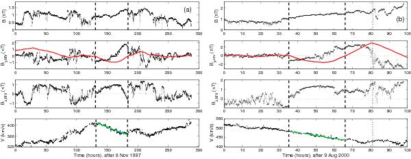
Examples of two MCs with velocity profiles that are not significantly perturbed (i.e. that have an almost linear dependence on time). a) MC 13 travels at low latitude (2°) at D = 5.3 AU in a slow SW and b) MC 30 travels at high latitude ( − 66°) at D = 3 AU in a relatively slow SW for such high latitude. The vertical dashed lines define the MC (flux rope) boundaries, and the vertical dotted line defines the rear boundary of the MC back (Sect. 2.3, a back is only present on the right panels). The three top panels show the magnetic field norm and its two main components in the MC frame computed with the MV method (Sect. 2.2). B_z,MV is the MC axial magnetic field component. B_y,MV is the magnetic field component both orthogonal to the MC axis and to the radial direction from the Sun (). The solid red line represents F_y, which is the accumulated flux of B_y,MV (Eq. (1)). The bottom panel shows the observed velocity component in the radial direction (). A linear least squares fit of the velocity (green line) is applied in the time interval where an almost linear trend is present within the MC.