| Issue |
A&A
Volume 542, June 2012
|
|
|---|---|---|
| Article Number | L29 | |
| Number of page(s) | 4 | |
| Section | Letters | |
| DOI | https://doi.org/10.1051/0004-6361/201219339 | |
| Published online | 05 June 2012 | |
Accounting for the XRT early steep decay in models of the prompt gamma-ray burst emission
UPMC-CNRS, UMR7095, Institut d’Astrophysique de Paris, 75014 Paris, France
e-mail: This email address is being protected from spambots. You need JavaScript enabled to view it.
; This email address is being protected from spambots. You need JavaScript enabled to view it.
; This email address is being protected from spambots. You need JavaScript enabled to view it.
;
Received: 4 April 2012
Accepted: 19 May 2012
Abstract
Context. The Swift-XRT observations of the early X-ray afterglow of GRBs show that it usually begins with a steep decay phase.
Aims. A possible origin of this early steep decay is the high latitude emission that subsists when the on-axis emission of the last dissipating regions in the relativistic outflow has been switched-off. We wish to establish which of various models of the prompt emission are compatible with this interpretation.
Methods. We successively consider internal shocks, photospheric emission, and magnetic reconnection and obtain the typical decay timescale at the end of the prompt phase in each case.
Results. Only internal shocks naturally predict a decay timescale comparable to the burst duration, as required to explain XRT observations in terms of high latitude emission. The decay timescale of the high latitude emission is much too short in photospheric models and the observed decay must then correspond to an effective and generic behavior of the central engine. Reconnection models require some ad hoc assumptions to agree with the data, which will have to be validated when a better description of the reconnection process becomes available.
Key words: gamma-ray burst: general / radiation mechanisms: non-thermal / radiation mechanisms: thermal / shock waves / magnetic reconnection
Institut Universitaire de France.
© ESO, 2012
1. Introduction
Thanks to its precise localization capabilities followed by rapid slewing, the Swift satellite (Gehrels et al. 2004) can quickly – typically in less than two minutes after a gamma-ray burst (GRB) trigger – repoint its X-ray Telescope (XRT, Burrows et al. 2005) toward the source. This achievement has helped to fill the gap in observationsbetween the prompt and late afterglow emissions and revealed the complexity of the early X-ray afterglow (Tagliaferri et al. 2005; Nousek et al. 2006; O’Brien et al. 2006). Despite this complexity, the early steep decay that ends the prompt emission appears to be a generic behavior, common to most long GRBs. During this phase, the flux decays with a temporal index α ≃ 3−5 (with Fν ∝ t − α). It lasts for a typical duration tESD ~ 102 − 103 s and is usually followed by the shallow or normal decay phases.
The rapid gamma-ray light curve variability suggests that prompt emission has to be produced by internal mechanisms (Sari & Piran 1997), while the later shallow and normal decay phases are usually attributed to deceleration by the external medium (e.g. Meszaros & Rees 1997; Sari et al. 1998; Rees & Meszaros 1998). As the backward extrapolation of the early steep decay connects reasonably to the end of the prompt emission, it is often interpreted as its tail. It has moreover been shown that it is too steep to result from the interaction with the external medium (see e.g. Lazzati & Begelman 2006).
One of the most discussed and natural scenario to account for the early steep decay had been described by Kumar & Panaitescu (2000) before the launch of Swift. It explains this phase by the residual off-axis emission – or high latitude emission – that becomes visible when the on-axis prompt activity switches off. This scenario gives simple predictions and several studies have been dedicated to check whether it agrees with observations (see e.g. Liang et al. 2006; Butler & Kocevski 2007; Zhang et al. 2007; Qin 2008; Barniol Duran & Kumar 2009). On the basis of a realistic multiple pulse fitting approach proposed by Genet & Granot (2009), Willingale et al. (2010) confirmed that the observed temporal slope of the early steep decay can be well explained in this context, while the accompanying spectral softening is (at least qualitatively) also reproduced.
In this Letter, we first discuss in Sect. 2 some constraints implied by the high latitude scenario on the typical radius Rγ where the prompt emission ends. We then investigate in Sect. 3 if they are consistent with the predictions of the most discussed models for the prompt phase: internal shocks, Comptonized photospheric emission, and magnetic reconnection. We summarize our results in Sect. 4, which also presents our conclusions.
2. Constraints on the prompt emission radius in the high latitude scenario
The high latitude interpretation of the early steep decay constrains the value of Rγ in two different ways:
-
(i)
The maximum possible duration of the high latitude emissiondepends on the opening angle θ of the jet and is given by
 (1)It has to be larger than the total duration of the early steep decay, tESD, which leads to (Lyutikov 2006; Lazzati & Begelman 2006)
  (2)
(2) -
(ii)
In a logarithmic plot where the the burst trigger is the origin of time, the high latitude emission has to behave as a power-law that smoothly connects to the end of the prompt phase with an initial decay index α ~ 3−5.
After the prompt emission ends at Rγ, the high latitude (bolometric) flux received by the observer has been derived by several authors (see e.g. Kumar & Panaitescu 2000; Beloborodov et al. 2011). It takes the form  (3)with
  (4)where Γ is the Lorentz factor of the emitting shell. In Eq. (3), tburst is the arrival time of the last on-axis photons, emitted at Rγ, and therefore corresponds to the duration of the prompt phase. The description of the flux given by Eq. (3) remains valid as long as a new emission component does not emerge leading to the shallow/normal decay phase of the afterglow. From Eq. (3), the initial temporal decay index of the high latitude emission equals
  (5)which implies that τHLE ≃ tburst to reproduce the observations, yielding a new constraint on Rγ
 (6)If conversely τHLE ≪ tburst (or Rγ ≪ R ∗ ), the high latitude flux will experience a huge drop (by a factor of about
  immediately after the prompt phase before recovering a slope α ~ 3 only after several tburst.
It should be noted however that Eq. (3) and the discussion that follows assume that the emitting surface at Rγ has a spherical shape and that the emission is isotropic in the comoving frame of the emitting material. This is not necessarily true (see Sect. 3 below) so that the constraints given by Eqs. (2) − (6) are only estimates that might be relaxed by a factor of a few, but certainly not by several order of magnitudes. We also note that the two constraints are compatible.
3. Comparison with the emission radii predicted in different GRB models
3.1. Internal shocks
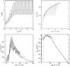 |
Fig. 1 Early steep decay from high latitude emission in the internal shock framework. Two examples of synthetic GRBs with a smooth (dashed line) or a highly variable (solid line) light curve. Top left: initial distribution of the Lorentz factor in the flow as a function of injection time tinj (a short timescale (0.5 s) fluctuation of the Lorentz factor is added to produce the variable burst). In the two cases, the injected kinetic power is constant. Top right: shock radius (smooth light curve case: thick line; variable light curve case: thin line) as a function of observer time, showing that the maximum values reached by the emission radius, i.e. Rγ, are comparable in the two cases. Bottom: bolometric light curve on either a linear (left panel) or logarithmic (right panel) scale. The high latitude contribution is very similar for both the smooth and variable light curves. |
It has sometimes been argued (e.g. Lyutikov 2006; Kumar et al. 2007) that the internal shock model (e.g. Rees & Meszaros 1994; Kobayashi et al. 1997; Daigne & Mochkovitch 1998) is incompatible with the high latitude scenario. The underlying argument is based on the assumption that internal shocks take place at a typical radius RIS estimated from the shortest variability timescale tvar,min observed in the prompt γ-ray light curve. In this simplified context, the inferred radius RIS ≃ 6 × 10¹³ (Γ/100)2 (tvar,min/0.1 s) cm is much too small compared to the high latitude scenario constraints given by Eqs. (2) − (6).
However, observed γ-ray light curves cover a wide range of variability timescales going from the shortest one tvar,min to the longest one tvar,max. The power density spectra of GRB light curves show that tvar,max is much longer than tvar,min and close to the whole burst duration tburst (see e.g. Beloborodov et al. 2000; Guidorzi et al. 2012). In the internal shock framework, the variability timescales in the light curve reflect those of the relativistic outflow. The initial Lorentz factor must then vary on timescales from tvar,min to tvar,max and the radius of the internal shocks extends from a minimum RIS,min ≃ 2Γ2ctvar,min to a maximum RIS,max ≃ 2Γ2ctvar,max, which is very close to R∗ ≃ 2Γ2ctburst. This implies that the the high latitude emission of the last internal shocks has a characteristic timescale τHLE ≃ tvar,max ≲ tburst, leading to a decay index α ≳ 3, in good agreement with XRT data. Internal shocks are therefore compatible with the requirements of the high latitude scenario even in highly variable bursts.
This result is illustrated by the synthetic GRBs shown in Figs. 1 and 2 where the dynamics of internal shocks has been computed with the multiple shell model of Daigne & Mochkovitch (1998). The example in Fig. 1 shows a mono-pulse burst (bottom left panel), either with (solid line) or without (dashed line) sub-structure. As seen from the initial distribution of the Lorentz factor (top left panel), the maximum variability timescale tvar,max is the same in both cases but the shortest variability timescale tvar,min is very different. The plot showing the location of the shocks (top right panel) clearly illustrates how the final radius – and therefore the high latitude emission – is governed only by tvar,max. The decay of the flux at the end of the prompt phase (bottom right panel) is therefore very similar in both cases, with a steep decay index reaching α ≃ 3 after a short and smooth transition. The example in Fig. 2 corresponds to a more complex light curve with three isolated pulses, where tvar,max ≃ tburst/3. The high latitude emission of each pulse is plotted as a dashed line. The final decay index of the total light curve is α ≃ 9 before reaching α ≃ 3 for tobs ≳ 2tburst (see also Genet & Granot 2009). We checked that adding substructure on shorter timescales does not affect this result. As a last example, the “naked burst” GRB 050421 is a good case of a GRB with a variable light curve followed by an early steep decay that was well observed by the XRT because of its especially long duration (Godet et al. 2006). This burst was modeled in detail by Hascoët et al. (2011). The prompt emission is associated with internal shocks and the high latitude emission is in excellent agreement with XRT data (see Fig. 2 in Hascoët et al. 2011).
We conclude from this analysis that the internal shock model naturally reproduces the XRT early steep decay phase in the high latitude scenario. We note that the value of α discussed above can be affected by two additional effects: (i) a spectral effect when the flux is integrated in a relatively narrow band (as in the case of Swift-XRT). The expected temporal decay slope is then α ≃ 2 + β, where the spectral slope β (Fν ∝ t − αν − β) can be larger than one; (ii) an emission that is already anisotropic in the comoving frame of the emitting material (e.g. Beloborodov et al. 2011). Finally, we limit our discussion to the bolometric flux for simplicity. If the peak energy of the spectrum radiated by the last internal shocks is above the spectral range of the XRT (i.e. above 10 keV), the peak energy of the high latitude emission crosses the XRT range, leading to spectral evolution during the early steep decay (see e.g. Genet & Granot 2009). This evolution is seen in many XRT observations (Zhang et al. 2007).
3.2. Photospheric emission
In photospheric models, the evolution of the high latitude flux is more complex than for a simple flashing sphere – the last scattering region has a finite width and is not spherically symmetric (with the last scattering radius increasing with latitude). However, a detailed calculation (e.g. Pe’er 2008; Beloborodov 2011) shows that the characteristic initial decay timescale remains τHLE ≃ Rγ/2Γ2c, where Rγ is now the photospheric radius Rph for on-axis photons. In the case of a “classical” non dissipative photosphere, Rph is given by (e.g. Piran 1999; Daigne & Mochkovitch 2002)  (7)where Ėiso is the isotropic equivalent kinetic power in the outflow, leading to
  (8)For standard values of the parameters τHLE ≪ tburst, so that the early steep decay cannot be explained by high latitude emission. Reducing the Lorentz factor at the photosphere to Γ ≲ 20 can increase Rph to an acceptable value but one is then confronted with a drop in the photospheric luminosity even before the high latitude emission sets in (since Lph ∝ Γ8/3, e.g. Mészáros & Rees 2000; Daigne & Mochkovitch 2002). The same conclusion holds (as Rph remains very close to the value given by Eq. (7)) in models where a dissipative process is invoked at the photosphere to transform the seed thermal spectrum into a non-thermal band spectrum (see e.g. Rees & Mészáros 2005; Beloborodov 2010).
In photospheric models, the early steep decay must therefore be directly produced by a declining activity of the central engine. This implies that a physical mechanism, common to most GRBs, governs the late activity in a generic way, in contrast to the diversity of the prompt gamma-ray light curves, which also reflect the activity of the central engine.
3.3. Magnetic reconnection
Gamma-ray burst models where the prompt emission comes from magnetic reconnection are still at an early stage of development and do not offer the same level of prediction as the two other families of models discussed above.
In a first situation investigated by Drenkhahn (2002), Drenkhahn & Spruit (2002), and Giannios (2008), the prompt emission is produced by a gradual reconnection process that begins below the photosphere and extends above. The dissipation process typically ends at a radius R ≃ 1013 cm, which remains too small for the high latitude scenario. In the model proposed by McKinney & Uzdensky (2012), reconnection remains inefficient below the photosphere before it enters a rapid collisionless mode at Rdiss ~ 1013 − 1014 cm and catastrophically dissipates the magnetic energy of the jet. This radius range becomes compatible with the high latitude scenario for GRBs of duration tburst ≃ 1 s but is still too small for most long GRBs. However, there are remaining theoretical uncertainties about the dissipation rate, and future calculations may predict a larger radius for the end of the reconnection process.
A full electromagnetic model was proposed by Lyutikov & Blandford (2003) where the energy is dissipated at large radii ( ≳ 1016 cm) when the interaction of an electromagnetic bubble with the shocked external medium becomes significant and current instabilities develop at the contact discontinuity. In this model, the gamma-ray variability is generated by the emission of “fundamental emitters” that are driven (by the dissipative process) into relativistic motion with random directions (some kind of relativistic turbulence) in the frame of the main outflow, which is also highly relativistic. Different authors have tentatively computed the expected bolometric light curves: in the examples presented by Lyutikov (2006), Lazar et al. (2009), and Narayan & Kumar (2009), the high latitude contribution smoothly connects to the end of a highly variable prompt phase. These results however require some degree of adjustment between different dynamical parameters. It is a priori decided that Rγ ≃ Γ2ctburst – which is not an intrinsic consequence of the model, in contrast to what happens with internal shocks.
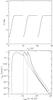 |
Fig. 2 Early steep decay from high latitude emission in the internal shock framework: a multi-pulse burst. Top: initial distribution of the Lorentz factor; Bottom: bolometric light curve on a logarithmic scale (solid line). The contribution of each individual pulse is plotted as a dashed line. |
Finally, in the model of Zhang & Yan (2011), a self-sustained magnetic process is triggered by prior internal shocks that are inefficient (because of a high degree of magnetization) but leave the magnetic field lines entangled. Some “dynamical memory” of the shocks is conserved and the conclusions of Sect. 3.1 basically apply. However, the details of the physical mechanisms involved in this model remain to be clarified and quantified.
4. Conclusion
The results of this Letter emphasize the importance of the steep decay phase revealed by Swift observations of the early X-ray afterglow. An attractive way of explaining this phase is to suppose that it is produced by the high latitude emission of the last contributing shells. We have shown that this assumption leads to strong constraints on the radius Rγ where the prompt emission ends. In particular, the associated timescale, τHLE ~ Rγ/2c Γ2 must be comparable to the burst duration tburst to guarantee that the high latitude contribution is correctly connected to the end of the prompt light curve. We have then checked whether these constraints are satisfied by different models for the prompt phase, namely internal shocks, Comptonized photospheric emission, and magnetic reconnection.
-
Internal shocks naturally fulfill the conditionτHLE ~ tburst even in highly variable bursts, as the radius of the last shocks is governed by the longest variability timescale, which is on the order of tburst.
-
Conversely, in photospheric models τHLE ≪ tburst, since the photospheric radius is typically several orders of magnitude smaller than the radius of internal shocks. The only way to produce the observed decay is then to suppose that it corresponds to an effective behavior of the central engine, which moreover should be common to most GRBs.
-
In magnetic reconnection models, satisfying the constraints on Rγ might be possible but is not naturally expected. It still requires the ad hoc assumption that Rγ ≃ Γ2ctburst, which will have to be justified when a better description of the reconnection process becomes available.
Acknowledgments
The authors acknowledge the French Space Agency (CNES) for financial support. R.H.’s Ph.D. work is funded by a Fondation CFM-JP Aguilar grant.
References
- Barniol Duran, R., & Kumar, P. 2009, MNRAS, 395, 955 [NASA ADS] [CrossRef] [Google Scholar]
- Beloborodov, A. M. 2010, MNRAS, 407, 1033 [NASA ADS] [CrossRef] [Google Scholar]
- Beloborodov, A. M. 2011, ApJ, 737, 68 [NASA ADS] [CrossRef] [Google Scholar]
- Beloborodov, A. M., Stern, B. E., & Svensson, R. 2000, ApJ, 535, 158 [NASA ADS] [CrossRef] [Google Scholar]
- Beloborodov, A. M., Daigne, F., Mochkovitch, R., & Uhm, Z. L. 2011, MNRAS, 410, 2422 [NASA ADS] [CrossRef] [Google Scholar]
- Burrows, D. N., Hill, J. E., Nousek, J. A., et al. 2005, Space Sci. Rev., 120, 165 [NASA ADS] [CrossRef] [Google Scholar]
- Butler, N. R., & Kocevski, D. 2007, ApJ, 663, 407 [NASA ADS] [CrossRef] [Google Scholar]
- Daigne, F., & Mochkovitch, R. 1998, MNRAS, 296, 275 [Google Scholar]
- Daigne, F., & Mochkovitch, R. 2002, MNRAS, 336, 1271 [NASA ADS] [CrossRef] [Google Scholar]
- Drenkhahn, G. 2002, A&A, 387, 714 [NASA ADS] [CrossRef] [EDP Sciences] [Google Scholar]
- Drenkhahn, G., & Spruit, H. C. 2002, A&A, 391, 1141 [NASA ADS] [CrossRef] [EDP Sciences] [Google Scholar]
- Gehrels, N., Chincarini, G., Giommi, P., et al. 2004, ApJ, 611, 1005 [NASA ADS] [CrossRef] [Google Scholar]
- Genet, F., & Granot, J. 2009, MNRAS, 399, 1328 [NASA ADS] [CrossRef] [Google Scholar]
- Giannios, D. 2008, A&A, 480, 305 [NASA ADS] [CrossRef] [EDP Sciences] [Google Scholar]
- Godet, O., Page, K., Osborne, J., et al. 2006, A&A, 452, 819 [NASA ADS] [CrossRef] [EDP Sciences] [Google Scholar]
- Guidorzi, C., Margutti, R., Amati, L., et al. 2012, MNRAS, 422, 1785 [NASA ADS] [CrossRef] [Google Scholar]
- Hascoët, R., Uhm, Z., Mochkovitch, R., & Daigne, F. 2011, A&A, 354, A104 [NASA ADS] [CrossRef] [EDP Sciences] [Google Scholar]
- Kobayashi, S., Piran, T., & Sari, R. 1997, ApJ, 490, 92 [NASA ADS] [CrossRef] [Google Scholar]
- Kumar, P., & Panaitescu, A. 2000, ApJ, 541, L51 [NASA ADS] [CrossRef] [Google Scholar]
- Kumar, P., McMahon, E., Panaitescu, A., et al. 2007, MNRAS, 376, L57 [NASA ADS] [Google Scholar]
- Lazar, A., Nakar, E., & Piran, T. 2009, ApJ, 695, L10 [NASA ADS] [CrossRef] [Google Scholar]
- Lazzati, D., & Begelman, M. C. 2006, ApJ, 641, 972 [NASA ADS] [CrossRef] [Google Scholar]
- Liang, E. W., Zhang, B., O’Brien, P. T., et al. 2006, ApJ, 646, 351 [NASA ADS] [CrossRef] [Google Scholar]
- Lyutikov, M. 2006, MNRAS, 369, L5 [NASA ADS] [CrossRef] [Google Scholar]
- Lyutikov, M., & Blandford, R. 2003, unpublished [arXiv:astro-ph/0312347] [Google Scholar]
- McKinney, J. C., & Uzdensky, D. A. 2012, MNRAS, 419, 573 [Google Scholar]
- Meszaros, P., & Rees, M. J. 1997, ApJ, 476, 232 [NASA ADS] [CrossRef] [Google Scholar]
- Mészáros, P., & Rees, M. J. 2000, ApJ, 530, 292 [NASA ADS] [CrossRef] [Google Scholar]
- Narayan, R., & Kumar, P. 2009, MNRAS, 394, L117 [NASA ADS] [CrossRef] [Google Scholar]
- Nousek, J. A., Kouveliotou, C., Grupe, D., et al. 2006, ApJ, 642, 389 [NASA ADS] [CrossRef] [Google Scholar]
- O’Brien, P. T., Willingale, R., Osborne, J., et al. 2006, ApJ, 647, 1213 [NASA ADS] [CrossRef] [Google Scholar]
- Pe’er, A. 2008, ApJ, 682, 463 [NASA ADS] [CrossRef] [Google Scholar]
- Piran, T. 1999, Phys. Rep., 314, 575 [Google Scholar]
- Qin, Y.-P. 2008, ApJ, 683, 900 [NASA ADS] [CrossRef] [Google Scholar]
- Rees, M. J., & Meszaros, P. 1994, ApJ, 430, L93 [NASA ADS] [CrossRef] [Google Scholar]
- Rees, M. J., & Meszaros, P. 1998, ApJ, 496, L1 [NASA ADS] [CrossRef] [Google Scholar]
- Rees, M. J., & Mészáros, P. 2005, ApJ, 628, 847 [NASA ADS] [CrossRef] [Google Scholar]
- Sari, R., & Piran, T. 1997, ApJ, 485, 270 [NASA ADS] [CrossRef] [Google Scholar]
- Sari, R., Piran, T., & Narayan, R. 1998, ApJ, 497, L17 [NASA ADS] [CrossRef] [Google Scholar]
- Tagliaferri, G., Goad, M., Chincarini, G., et al. 2005, Nature, 436, 985 [NASA ADS] [CrossRef] [PubMed] [Google Scholar]
- Willingale, R., Genet, F., Granot, J., & O’Brien, P. T. 2010, MNRAS, 403, 1296 [NASA ADS] [CrossRef] [Google Scholar]
- Zhang, B., & Yan, H. 2011, ApJ, 726, 90 [NASA ADS] [CrossRef] [Google Scholar]
- Zhang, B.-B., Liang, E.-W., & Zhang, B. 2007, ApJ, 666, 1002 [NASA ADS] [CrossRef] [Google Scholar]
All Figures
|
Fig. 1 Early steep decay from high latitude emission in the internal shock framework. Two examples of synthetic GRBs with a smooth (dashed line) or a highly variable (solid line) light curve. Top left: initial distribution of the Lorentz factor in the flow as a function of injection time tinj (a short timescale (0.5 s) fluctuation of the Lorentz factor is added to produce the variable burst). In the two cases, the injected kinetic power is constant. Top right: shock radius (smooth light curve case: thick line; variable light curve case: thin line) as a function of observer time, showing that the maximum values reached by the emission radius, i.e. Rγ, are comparable in the two cases. Bottom: bolometric light curve on either a linear (left panel) or logarithmic (right panel) scale. The high latitude contribution is very similar for both the smooth and variable light curves. |
| In the text | |
|
Fig. 2 Early steep decay from high latitude emission in the internal shock framework: a multi-pulse burst. Top: initial distribution of the Lorentz factor; Bottom: bolometric light curve on a logarithmic scale (solid line). The contribution of each individual pulse is plotted as a dashed line. |
| In the text | |
Current usage metrics show cumulative count of Article Views (full-text article views including HTML views, PDF and ePub downloads, according to the available data) and Abstracts Views on Vision4Press platform.
Data correspond to usage on the plateform after 2015. The current usage metrics is available 48-96 hours after online publication and is updated daily on week days.
Initial download of the metrics may take a while.