| Issue |
A&A
Volume 542, June 2012
|
|
|---|---|---|
| Article Number | A107 | |
| Number of page(s) | 10 | |
| Section | Astronomical instrumentation | |
| DOI | https://doi.org/10.1051/0004-6361/201218958 | |
| Published online | 14 June 2012 | |
On the calibration of full-polarization 86 GHz global VLBI observations
1 Max-Planck-Institut für Radioastronomie (MPIfR), Auf dem Hügel 69, 53121 Bonn, Germany
2 Onsala Space Observatory, Chalmers University of Technology, Observatorievägen 90, 43992 Onsala, Sweden
e-mail: ivan.marti-vidal@chalmers.se
3 Institute for Astrophysical Research, Boston University, 725 Commonwealth Avenue, Boston, MA-02215, USA
4 Institute of Geodesy and Geoinformation, Bonn University, Nussallee 17, 53115 Bonn, Germany
5 Institut de Radioastronomie Millimétrique (IRAM), 300 rue de la Piscine, 38406 Saint Martin d’ Hères, France
6 Instituto de Radioastronomía Milimétrica (IRAM), Av. Divina Pastora 7, Núcleo Central, 18012 Granada, Spain
7 Metsähovi Radio Observatory (Aalto University), Metsähovintie 114, 02540 Kylmälä, Finland
Received: 3 February 2012
Accepted: 7 March 2012
We report the development of a semi-automatic pipeline for the calibration of 86 GHz full-polarization observations performed with the Global Millimeter-VLBI array (GMVA) and describe the calibration strategy followed in the data reduction. Our calibration pipeline involves non-standard procedures, since VLBI polarimetry at frequencies above 43 GHz has not yet been well established. We also present, for the first time, a full-polarization global-VLBI image at 86 GHz (source 3C 345), as an example of the final product of our calibration pipeline, and discuss the effect of instrumental limitations on the fidelity of the polarization images. Our calibration strategy is not exclusive to the GMVA, and could be applied to other VLBI arrays at millimeter wavelengths. The use of this pipeline will allow GMVA observers to obtain fully calibrated datasets shortly after the data correlation.
Key words: instrumentation: interferometers / techniques: interferometric / radio continuum: general
© ESO, 2012
1. Introduction
The Global Millimeter-VLBI array (GMVA) is the result of a collaboration of a group of radio observatories, led by the Max-Planck-Institut für Radioastronomie (MPIfR), interested in performing astronomical very-long-baseline interferometry (VLBI) observations at millimeter wavelengths1. The GMVA currently consists of the radio telescopes at Effelsberg (100 m, MPIfR, Germany), Pico Veleta (30 m, IRAM, Spain), Plateau de Bure (six 15 m antennas working in phased-array mode, IRAM, France), Onsala (20 m, Sweden), Metsähovi (14 m, Finland), and a subset of the Very Long Baseline Array2 (i.e., all the VLBA antennas equipped with 86 GHz receivers, which are those at Brewster, Owens Valley, Mauna Kea, Pie Town, Kitt Peak, Fort Davis, Los Alamos, and North Liberty). Some technical details of these antennas are given in Table 1. Additional antennas (e.g., the 40 m telescope at Yebes Observatory, Spain; the NRAO 100 m Green Bank Telescope, USA; the 50 m Large Millimeter Telescope, LMT, Mexico; the 64 m Sardinia Radio Telescope, SRT, Italy; and, later, the Atacama Large mm-submm Array, ALMA, Chile) are planned to join the global 3 mm-VLBI effort in the future. Owing to its large number of participating telescopes and a coordinated observing strategy, based on an efficient observing-time allocation, the GMVA is capable of providing high quality images of high spatial resolution (40−70 μas) at 86 GHz. On its most sensitive baselines (i.e., to the IRAM and Effelsberg telescopes), the GMVA offers a ~3−4 times higher sensitivity and a ~2 times higher angular resolution than the stand-alone VLBA. This makes it possible to obtain detailed high angular resolution and high quality images of emission regions that appear self-absorbed (and are therefore invisible) at lower frequencies. The very high spatial resolution achievable with the GMVA is crucial to our understanding of high-energy astrophysical phenomena, e.g. physical processes in active galactic nuclei (AGN) and in the vicinity of supermassive black holes.
Technical details of the GMVA stations.
In this paper, we describe the steps required to calibrate GMVA observations, from the subband phase calibration (i.e., the alignment of phases and delays in the different observing subbands) to the global fringe fitting (GFF; Schwab & Cotton 1983) and the polarization calibration. This paper focuses only on the technical aspects of the data calibration and reduction, which at millimeter wavelengths deviates in some details from the standard data analysis that is typically applied at longer cm-wavelengths. The scientific exploitation of the data is of course a matter of the principal investigators (PIs) of the projects approved for GMVA observations.
A special motivation for this paper is that VLBI polarimetry at frequencies above 43 GHz is neither standard, nor well-established. Extending the frequency coverage of VLBI polarimetry to higher frequencies is important to obtain a clearer understanding of the details in jet physics (e.g. Homan et al. 2009; O’Sullivan et al. 2011; Gómez et al. 2011) or the origin and launching mechanisms of jets near the central black hole in AGN (e.g., Broderick & Loeb 2009; Tchekhovskoy et al. 2011; Mc Kinney et al. 2012). We therefore believe that it is important to discuss the possibilities and limitations of polarimetric VLBI observations at mm-wavelengths, which so far have not yet been fully exploited. There are only a few published 86 GHz polarization images (e.g. Attridge 2001; Attridge et al. 2005; Gómez et al. 2011), which were made using the VLBA only, and not the global, and more sensitive, 3 mm-VLBI array.
We present as an example of our calibration strategy results obtained from part of the full-polarization observations taken in the GMVA session in May 2010. We also present some representative images (in total intensity and polarization) of the quasar 3C 345 (one of the sources observed in that session). In Sect. 3, we summarize the technical details of the observations. In Sects. 4 to 6, we depict the calibration strategy in chronological order: the whole phase calibration is described in Sect. 4, the amplitude calibration is described in Sect. 5, and the correction for the polarization leakage at the receivers is described in Sect. 6. Finally, we present sample images of 3C 345 in Sect. 7 and summarize our work in Sect. 8.
2. Observing with the GMVA
For logistical reasons, the GMVA observations are performed in four-to-six day-long sessions twice per year (in spring and autumn) and the call for proposals shares the deadlines with those of the VLBA (i.e., February 1 and August 1 each year). The proposals are refereed individually by the participating institutes, and the ratings are then combined to determine the projects to be observed.
For each observing session, the experiments belonging to different principal investigators (PIs) are combined into a single VLBI observing time block at all telescopes. Within this block time, the detailed observing schedule may be sub-divided into different scheduling blocks arranged to minimize the idle times of the telescopes and maximize the uv-plane coverage for the observed radio sources within the given time constraints. Hence, when a source is not visible to the whole interferometer (because of the different rise and setting times between the USA and Europe), the scheduling strategy includes sub-arraying (i.e., division of the whole GMVA into two or more independent arrays). The use of subarrays allows the schedulers to optimize on-source integration times and antenna elevations, but also causes some difficulties in the data calibration and reduction. For instance, it is not always possible to assign a common reference antenna for the GFF. Hence, the calibration of phase-like quantities (phases, delays, and rates) requires a continuous re-referencing between the subarrays, which may often change during the GMVA session.
Nevertheless, all the peculiarities in the data calibration caused by the complex structure of GMVA schedules should not present any problem for the PIs, since the bulk of the data calibration and editing could be performed at the VLBI correlator and data analysis center (e.g. at the MPIfR), following the steps described in this paper.
3. GMVA observations on May 2010
This paper concerns, as a test dataset, the GMVA observations conducted between the 6 and the 11 of May 2010. Most of the observing session was performed in dual-polarization mode (i.e., the left circular polarization, LCP, and the right circular polarization, RCP, were simultaneously observed) at a frequency of 86 GHz, with an overall recording rate of 512 Mb s-1, 2-bit sampling in Mark5B format. Four 16 MHz subbands were used at each polarization. For each subband, the correlator produced 32 spectral channels. In the correlation process, all possible combinations of the polarizations were correlated, to yield all four Stokes products.
The full set of GMVA antennas participated in these observations. The observations were divided into scans of about seven minutes. There were a total of 18 AGN observed with different overall on-source times.
4. Phase calibration
The phase calibration is the most critical and time-consuming part of the data reduction, especially at 86 GHz, because of strong atmospheric and instrumental phase instabilities. The full process of phase calibration (with the exception of the eventual phase self-calibration involved in the source imaging) was performed using the NRAO Astronomical Image Processing System (AIPS). We used AIPS in batch mode by writing several scripts in ParselTongue (a Python interface to AIPS; see Kettenis et al. 2006). This process involves the following main steps:
-
Preliminary calibration. We corrected the effect of the changing parallactic angle of each antenna. The effects of the Nasmyth mount of the Pico Veleta station were also corrected (see Dodson 2009).
-
Subband phase calibration. The independent oscillators of the single-sideband mixers introduce unknown phase offsets in each subband. In addition, owing to the different lengths of the signal paths, there may be slightly different delays and phases among the subbands at each station. These delays and phases were defined with respect to one (reference) antenna.
-
Global fringe-fitting on the multi-band data. We estimated the antenna-dependent multi-band gains (i.e., delays, phases, and phase rates, over the whole band) for all the observations.
-
Polarization calibration. We found the delay and phase difference between subbands in the cross-hand (i.e., RL and LR) correlations.
4.1. Subband phase calibration
A common strategy for the correction of the different delays and phases of the subbands is to use the so-called phase-cal injection tones, which are sharp pulses injected in the signal path, close to the receiver horn. However, this approach is impossible for the GMVA, since the 86 GHz receivers of the VLBA do not have phase-cal injection tones. In addition, the phase-cal tones at the European telescopes are not injected at the receiver front-end, but at a later stage in the signal path. Hence, there may be instrumental phase variations in the signal that cannot be corrected from the phase-cal tones; these variations can only be removed via the alternative manual phase-calibration approach.
With a manual phase-calibration, the unknown delays and phases among subbands are estimated from the application of the GFF algorithm to a set of visibilities from a bright source. Independent solutions for the delay and phase of each subband, antenna, and polarization are found from the observations. The delay and phase solutions for that particular subset of visibilities are then extrapolated to the whole dataset. The antenna-dependent phase solutions computed with the GFF algorithm must be referred to a so-called reference antenna, to which is assigned, by definition, a zero phase (and delay) gain.
However, the manual phase-calibration may lead to an imperfect alignment of the phases among the subbands, mainly due to possible drifts in the electronics of the receiving systems during the relatively long duration of a GMVA session. Moreover, the many subarraying conditions present in the GMVA observations make it impossible to assign the same reference antenna to the whole dataset. In addition, it is difficult to find scans of bright sources simultaneously observed with the whole interferometer, since weather or station-related problems may cause missed calibrator observations; furthermore, the calibrators are quite variable at 86 GHz, so it is not easy to select the most suitable calibrator sources at the time of the schedule preparation. Our script for the calibration of GMVA observations overcomes these drawbacks of manual phase-calibration in the following way:
-
1.
The script performs the GFF (using the AIPS task FRING) to the whole set of observations. It finds independent solutions for the phases and delays of each subband and polarization. Different reference antennas may be used by FRING if the main reference antenna (e.g., Los Alamos) is missing in a particular subarray and/or time. We note, though, that any change of reference antenna made by FRING does not affect our final calibration (see below).
-
2.
From all the FRING solutions, the script filters only those with the highest signal-to-noise ratio (S/N). A typical cut-off is S/N ≥ 20.
-
3.
The remaining solutions are arranged in terms of both the antenna and reference antenna, and the delays and phases are referred to those of a given (reference) subband and polarization. (i.e., the phase and delay differences between subbands are calculated, in order to remove these purely instrumental contributions from the data).
-
4.
The resulting delay and phase differences of each antenna are binned using a median-window filter (MWF) and the bins are linearly interpolated in time. Different averaging and interpolation schemes may be applied and visually checked, until a satisfactory time interpolation of the phases and delays at all the antennas is obtained.
-
5.
The interpolated phases and delays are applied to the whole dataset and re-referenced, when necessary, to the main (i.e., the most commonly appearing) reference antenna.
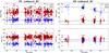 |
Fig. 1 Single-band phases (upper figures) and delays (lower figures) in the second subband of Fort Davis (left) and Plateau de Bure (right), referred to Los Alamos, for both circular polarizations. Times are given in day of the year (DOY). The gains are referred to the first subband in the LCP polarization. Solid lines are the interpolations applied to calibrate the data. Note that these plots show data for all sources. |
In addition, this approach does not assume that the phase and delay differences between subbands remain constant during the whole session, but allows us to check for any drift in the electronics of the receivers. We show in Fig. 1 some representative plots generated with our script. The subband used as reference was the one corresponding to LCP and the lowest sideband frequency. For the case of Fort Davis (antenna code FD), it can be seen that the phases (with an average of 10.3 ± 0.9 deg for LCP and −53.1 ± 0.3 deg for RCP) and delays (with an average of 29.09 ± 0.18 ns for LCP and 10.45 ± 0.10 ns for RCP) remain remarkably constant, as is also the case for most of the antennas. However, a drift is seen in the phases of the second subband of Plateau de Bure (antenna code PB) for the RCP polarization (average phase of 6.07 ± 5.01 deg for LCP; 124.4 ± 68.6 deg for RCP). The overall drift in this subband is larger than 50 deg through the whole session, which translates into an average drift of ~10 deg per day. Since PB is a phased array, the drift seen in Fig. 1 may be due to the signal pre-processing before arriving at the recording system, although similar drifts have been found at other antennas (e.g., Effelsberg) during the ongoing analysis of other GMVA observations (not reported here). We are currently analyzing in greater detail the possible reason for these unexpected phase drifts between subbands.
4.2. Fringe fitting
Once the manual phase calibration has been performed to yield a higher sensitivity, it is possible to combine the data from all the subbands and estimate the (multi-band) phases, delays, and rates for each antenna, source, and time. This step is the so-called multi-band fringe fitting.
Since we usually deal with weak sources (in terms of the sensitivity of the antennas) and the coherence time of the signals is relatively short (owing to the rapidly changing atmosphere at high frequencies), it is not straightforward to select the optimal combination of parameters for the fringe-fitting algorithm. On the one hand, a short coherence time calls for short integration times, to avoid a reduction in amplitude. This is so because non-linear drifts in the phase would degrade the fringes, thus broadening (or even smearing out) the fringes. On the other hand, a short integration time reduces the chance of a successful fringe detection.
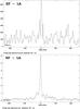 |
Fig. 2 Fringe-rate spectra at the baselines of Effelsberg to Los Alamos (EF-LA, baseline of 7831 km) and Kitt Peak to Los Alamos (KP-LA, baseline of 752 km), for an observation of source 3C 273B with an integration time of four minutes. |
We estimated the optimal integration time to be used on GMVA data by analyzing the performance of the GFF for different integration times. For an integration time of 3–4 min, the number of good (i.e., high S/N) solutions is maximized with respect to bad, or failed, ones. Since an integration time of 3−4 min is much longer than the actual (expected) atmosphere coherence time at 86 GHz (i.e, ~10−20 s), our results indicate that the changes in the fringe rate caused by the atmosphere are not so severe and/or systematic as to break down the phase coherence during an integration time longer than the expected ~10−20 s, although the exact coherence time will depend, of course, on the weather conditions at each station (humidity, wind speed, etc.). In other words, the phase fluctuations are centered mostly around an average slope (on a timescale much longer than that of the wrapping of the phase, for reasonably good weather conditions). Hence, if we apply the GFF using long integration times, we will be able to estimate and remove the main slope in the time evolution of the visibility phases, thus improving the signal coherence (see, e.g., Rogers et al. 1984; Baath et al. 1992; and Rogers et al. 1995, for additional discussions on the phase coherence in high-frequency VLBI observations). As an example of the quality in the coherence of the GMVA phases, Fig. 2 shows the fringe-rate spectra at two baselines (Effelsberg to Los Alamos and Kitt Peak to Los Alamos) for an observation of source 3C 273B, with an integration time of four minutes. We note the sharp peaks in the fringe rates after such a long integration time (and especially for EF-LA, which is one of the longer baselines).
On the basis of these results, our script for the GMVA calibration uses a mixed approach, to optimize the performance of the GFF. First, a preliminary fringe fitting is executed using a long integration time (four minutes) and a low S/N cut-off (S/N > 4.5). The script then reads the estimated antenna delays and bins them in time using a median window filter. Finally, the script averages and interpolates the bins and applies the interpolated delays to the whole dataset. We note that the bulk of the multi-band delays is expected to depend only on the antennas, and be almost independent of source structure. Hence, it is reasonable to homogeneously apply the delays interpolated by our script to the visibilities of all the observed sources. Given that we perform the manual phase calibration by referring the phases and delays of one polarization to those of the other, it is indeed expected that the remaining multi-band delays will be very similar for the LCP and the RCP data. We show in Fig. 3, the multi-band delays computed by FRING for the baseline of Brewster to Los Alamos. The figure clearly shows how the delays are very similar for the different sources, and both polarizations, throughout GMVA session.
This initial estimate of the antenna delays allows us to perform a second fringe fitting with a shorter solution interval (of about two minutes), but using a much narrower window for the delay search (1–10 ns, depending on the scatter in the delay solutions inferred from the first fringe-fitting run). Since the integration time in the second fringe-fitting run is shorter, the resulting rates and phases will more closely follow the behavior of the rapidly changing atmosphere over each antenna.
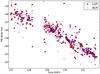 |
Fig. 3 Multi-band delay between the antennas at Brewster and Los Alamos vs. time. Notice that data of all sources have been included in this plot. |
The script then tries to recover the fringes that could not be found in the previous runs of FRING. It identifies all the combinations of antennas, sources, and times for which there were no FRING solutions. These data are then pre-calibrated, using a linear interpolation of the nearby FRING solutions, and a new iteration of FRING is run. However, this time, only the failed antennas of each scan are included in the fit. This approach could be understood as a robust iteration in the fringe search, which minimizes the number of discarded (i.e., edited) visibilities, although a lower S/N cut-off (~3.5) is necessary to decrease the number of failed solutions (by 15–20%). The overall amount of visibilities lost because of the non-detected fringes is ~10–20%, for an S/N cut-off of 4–5 (for this particular dataset).
As a final step, the script corrects for the effect of the slightly different rates and delays found by FRING between the RR and LL correlations. Even a small difference in the rate of only a few mHz between the RR and LL correlations may translate, after the calibration, into undesired drifts in the RL and LR phases between subbands, thus making it very difficult afterwards to perform a reliable correction of the instrumental polarization (see next section).
4.3. Polarization calibration
At this stage in the data calibration, all the subband phases and delays in the parallel-hand visibilities (i.e., the LL and RR correlations) are aligned, as described in Sect. 4.1, and the residual multi-band delays, phases, and rates are fitted and calibrated out, as described in the previous section. The only remaining instrumental effects in the data are due to the instrumental polarization. On the one hand, there are still delay and phase differences between the subbands of the the cross-hand correlations; on the other hand, there is a polarization leakage in the receivers of the antennas that must be estimated and corrected. Calibration of the polarization leakage is described in Sect. 6. In the present section, we describe the procedure used to calibrate the remaining delay and phase differences between the subbands of the cross-hand (i.e., RL and LR) correlations.
Any difference between the path of the RCP and LCP signals at the main reference antenna (i.e, the antenna with null phase gains after the manual phase calibration described in Sect. 4.1) maps into a phase and delay difference in the subbands of the cross-hand correlations. With the lack of useful phase-cal tones, this difference can only be corrected if the cross-hand correlations are fringe-fitted. Our script for the calibration of GMVA observations makes use of the AIPS task BLAVG to average the cross-hand correlations of all the baselines related to the reference antenna, and exports them to a separate file. The script then runs FRING on the visibilities contained in that file and the AIPS task POLSN is applied to the FRING output (POLSN refers all the solutions of one polarization to the other, and applies the resulting gains to all antennas.) Finally, the script filters out the gains of scans with a low S/N (lower cut-off of S/N ≤ 7), bins the remaining gains using a median window filter, and interpolates between bins.
We show in Fig. 4 the cross-hand phases and delays found by FRING (and re-referenced by POLSN) for the dataset reported here. These quantities are stable during the whole observing session, although we note that this stability is found as long as the rates applied to the calibration of the LL and RR correlations (i.e., the rates found by the GFF as described in Sect. 4.2) are always set to be equal3. It is indeed expected that the rates depend only on the source coordinates, station position, and clock models, which are equal for both polarizations. If we were to calibrate the data using the rates estimated by the fringe fitting, the small differences that might appear between the RR and LL correlations (because of the effects of noise in the fringe search) would introduce phase-drifts and delay differences into the signals of the RCP and LCP subbands of the main reference antenna, thus preventing the polarization calibration.
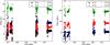 |
Fig. 4 Left, delay differences between LCP and RCP at Los Alamos. Right, phase differences at the same station (referred to those in the subband at the lowest frequency, IF1). |
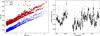 |
Fig. 5 Left, system temperatures (Tsys) measured at Los Alamos vs. airmass. Straight lines are fits of linear models to the lower envelopes of the Tsys distributions. The receiver temperature is estimated as the extrapolation of the lower envelope to a null airmass. Right, zenith opacity (i.e., opacity multiplied by the sine of the antenna elevation) at Los Alamos vs. time, as estimated using Eq. (1). |
5. Amplitude calibration
At high radio frequencies, the atmospheric absorption becomes significant (signal attenuations of 10 or 30% are not uncommon at 86 GHz). Hence, the atmospheric opacity must be taken into account in the amplitude calibration of the GMVA data. The atmospheric opacity τ is estimated at each station (and for each time) using the well-known formula 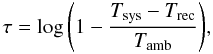 (1)where Tsys is the (opacity-uncorrected) system temperature and Trec is the temperature of the receiver. In this equation, it is assumed that the sky temperature (i.e., Tsys − Trec) is equal to the average temperature of the atmosphere (Tamb) corrected by the absorption factor exp(τ). The spill-over correction and the antenna temperature due to the source are very small quantities (less than a few K), hence can be neglected. When a noise diode is used for the signal calibration, Tsys is directly measured at the backend of each antenna receiver. In contrast, if the calibration strategy is based on a chopper wheel, the system directly measures the opacity-corrected system temperature (i.e., Tsysexp(τ)). In any case, the ambient temperature, Tamb, can be estimated from the weather monitoring at each station and the receiver temperature, Trec, can be estimated from the data, assuming that it is a stable quantity (on a timescale of one day or more).
We estimate the receiver temperature for each station (and polarization) by fitting the lower envelope of the Tsys vs. airmass distribution with a linear model. The extrapolation of that model to a null airmass then gives us a reliable estimate of the receiver temperature in the time range considered. We show in Fig. 5 (left) a sample plot of Tsys vs. airmass, together with the fit to the lower envelope, for the Los Alamos station. It can be seen in the figure that the receiver temperature differs slightly for each polarization. However, we note that our script forces the slopes of the lower envelopes to be the same at both polarizations (since the contribution of the atmosphere to Tsys is independent of the polarization). We show in Fig. 5 (right) the resulting time evolution of the opacity at zenith (i.e., corrected for the sine of the elevation) at Los Alamos. Once the opacity is known, the corrected system temperature, T∗, is easily computed as 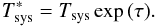 (2)There may be cases where an opacity correction had already been applied to the Tsys values provided by a given station (e.g., Plateau de Bure, Pico Veleta, or Onsala). In these cases, a differential (or refined) opacity correction can still be applied using the approach described here4. There is also the possibility of applying a constant (zenith-)opacity correction to the antennae where it is impossible to find precise estimates of the receiver temperature. In any case, our goal in the processing of each GMVA dataset is to provide the end user with a calibration table including all the opacity-corrected gains, as well as a set of AIPS-friendly files with all the
  estimates (i.e., the opacity-corrected temperatures) and the original Tsys values measured at each station (in case the user would like to apply a different approach to correct for the atmospheric opacity).
6. Polarization leakage
The LCP and RCP signals from the sources are separated in the frontend of the receivers, and follow different paths in the electronics. However, the receivers are imperfect, and there is a certain level of cross-talk between the RCP and LCP signals. The RCP (LCP) signal recorded at each station is thus equal to the true RCP (LCP) signal from the source, plus an unknown fraction of LCP (RCP) signal modified by a phase gain. The (complex) factors that account for the fraction of LCP (RCP) source signal transferred to the recorded RCP (LCP) signals are the so-called D-terms, which may differ at each antenna and for each polarization (for an in-depth discussion of the polarization leakage and its correction using the D-term approach, see Leppänen et al. 1995). The antenna D-terms are expected to depend only on the station hardware, and be stable quantities over periods of the order of one year (Gómez et al. 2002), although this may depend on the observing frequency. In this section, we describe how the D-terms are estimated, and how their effects are corrected in the GMVA observations.
Once the data are calibrated in both phase and amplitude, we perform a deep hybrid imaging with the program Difmap (Shepherd et al. 1994), by applying phase and amplitude self-calibration under reasonable limits, and taking special care with noisier data (since, in these cases, there may be a high probability of generating spurious components in the source structures; e.g., Martí-Vidal & Marcaide 2008). To ensure optimal results, all the hybrid imaging is performed without scripting.
The final images and calibrated data are then read back into AIPS by the script, source by source. The AIPS task CALIB is executed to perform the correction of any possible RCP-to-LCP amplitude bias at the antennas (by assuming a zero circular polarization for all the sources). The CLEAN components corresponding to the main features in the structure of each source are then combined with the AIPS task CCEDT (the regions defining the main features in the source structures have already been selected manually, after the hybrid imaging). Finally, the task LPCAL estimates the D-terms of each antenna, as well as the polarization of the different source components.
We note that the accuracy of the D-term determination depends on the strength of the detected cross-polarized signal, which may be higher if the source is strongly polarized or the antenna has strong intrinsic cross-polarization (but it should be below of 10%, to avoid problems with the linear approximation used in LPCAL). The accuracy also depends on the uniformity and range of the parallactic angle coverage and, to a lesser extent, also on the complexity of the polarized source sub-structure.
6.1. D-terms and image fidelity
Since the D-terms are estimated using the data of each source separately, we have as many estimates of antenna D-terms as sources (we consider the possibility of fitting one single set of D-terms to the visibilities of all sources, simultaneously, which would result in a more robust modeling of the polarization leakage). The final D-terms that we apply to each antenna are a weighted average of all estimated D-terms. Prior to the average, any clear outliers are removed, and the relative weights are adjusted as a function of the source flux density (and its fraction of polarized emission); the stronger the signal of the source in the cross-hand correlations, the higher the weight of the corresponding D-terms in the average. This approach is very similar to those reported in previous publications discussing high-frequency VLBI polarimetry (e.g. Marscher et al. 2002).
We give the average D-term amplitudes of all the antennas in Table 1 (Col. 6). We note that the dispersion in the D-terms estimated from the visibilities of the different sources is large (see the uncertainties in the amplitude averages!). Such a large dispersion in the D-term estimates is indicative of a strong coupling (in the LPCAL fitting) between the polarization leakage and the polarized source components, which maps into a poor modeling of the polarization leakage. We also note that the visibilities in the cross-hand correlations are quite sensitive to the leakage, so the final full-polarization GMVA images may differ notably, depending on the different schemes used for the estimate of the D-terms.
However, we expect that the main polarization features in the images (i.e., the source components with the strongest polarized emission) are rather insensitive to changes in the estimated D-terms. Moreover, there may also be correlations between the D-terms (i.e., couplings in the D-term estimates at the different antennas, resulting from the fitting procedure in LPCAL), such that images obtained from the use of different sets of D-terms do not differ significantly. We performed a quantitative analysis of how strongly the GMVA polarization images differ as a function of the different weighting schemes in the D-term averaging. In our analysis, we estimated the highest dynamic range achievable in the polarization images, such that the result should be nearly independent of the weights applied in the D-term averaging. This analysis is based on a Monte Carlo approach, and is described in the following lines. For each source:
-
1.
we generate the dirty image of the Stokes parameters Q and U, calibrated using the vector-averaged D-terms (which are obtained as described in Sect. 6). We call this result the reference polarization image;
-
2.
we compute a new vector-average of the D-terms, but using random weights for the different sources (weights uniformly distributed between 0 and 1);
-
3.
we generate the dirty images of the Stokes parameters Q and U using these new D-terms, and subtract these images from the reference image (i.e., that generated in step 1). We call these results differential polarization images;
-
4.
we compute the ratio of the intensity peaks in the differential images (i.e., those generated in step 3) to the intensity peak in the reference image (i.e., that generated in step 1);
-
5.
we iterate steps 2 to 4.
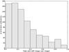 |
Fig. 6 Distribution of the intensity peaks of the differential polarization images (see text) of source 3C 345, after dividing by the peak of the reference polarization image. |
In Fig. 6, we show the distribution of intensity peaks in the differential polarization images of source 3C 345, using a total of 1000 Monte Carlo iterations. The cut-off probability of 95% (i.e., 2 sigma) for the null hypothesis of a false detection corresponds to a peak intensity of ~0.65 times the peak in the polarization image. Hence, any source component with a flux density higher than ~0.65 times that of the peak can be considered as real, with a confidence of 95%.
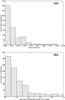 |
Fig. 7 a) Distribution of the shifts in the intensity peaks of all the polarization images obtained in our Monte Carlo D-term analysis. b) Same as Fig. 6, but taking into account the peak shifts before computing the differential polarization images. |
The images obtained using different D-terms do not only differ in terms of the strength of the polarized features, but also in their location. Many of the Monte Carlo iterations for which we found large peaks in the differential images correspond to cases where the peaks of the Monte Carlo images were slightly shifted with respect to the peak of the reference polarization image. We show in Fig. 7a the distribution of shifts between the peak of the reference image and the peak of the images obtained for all the Monte Carlo iterations. In most of the Monte Carlo images, the peaks are at less than 30 μas away from the peak of our reference polarization image (this is roughly the size of the minor axis of our beam). If we take into account these small shifts in the computation of the differential polarization images, the resulting peaks of the new differential images are somewhat lower than those obtained without shifting, as we show in Fig. 7b. Hence, if the small shifts are corrected, the final images typically do not differ by more than 50–60% of the source peak (with a confidence interval of 95%). The position shifts obtained from the different D-term calibration also imply that the astrometric precision of the location of the polarized emission is on the order of ~30 μas (roughly the size of the minor axis of the synthesized beam).
7. Representative images
After the data have been calibrated as described in the previous sections, they are ready for a full-polarization imaging, taking into account the polarization limitations described in Sect. 6.1. We present, in Fig. 8, a sample image of the source 3C 345 obtained from the GMVA observations reported here. The high quality of the GMVA data allows us to recover an extended jet structure that is distant from the core, after careful imaging including iterative amplitude self-calibration and uv-tapering. We also show in Fig. 9 two polarization images of the same source, obtained from different estimates of the antenna D-terms (i.e., averaging the D-terms estimated from the visibilities of a selection of sources or using the D-terms just estimated from the visibilities 3C 345). The polarization is very similar in both images (we applied a cut-off at 60% of the polarization peak). There is polarized emission at the north-east side of the core, where the electric-vector position angle (EVPA) is perpendicular to the jet. The electric vector position angle then rotates as the distance to the core increases westwards. The polarization images in Fig. 9 can be compared to another image obtained from VLBI observations at 43 GHz (Jorstad et al., in prep.) taken on 19 May 2010, only a few days before our GMVA session. We show the 43 GHz image (only the part near the VLBI core of the source) in Fig. 10. The electric vector position angle at 43 GHz is very similar to that of the optically-thin components in Fig. 9 (i.e., the western components, away from the core at 86 GHz), although we note that the absolute electric-vector position angle (i.e., a possible global R-L phase offset at the reference antenna, which would map into a global rotation of all the polarization vectors in the image) was not determined for our observations. We also note that the polarized core component with a north-south electric-vector position angle at 86 GHz is not detected at 43 GHz. Possible reasons for this discrepancy in the polarized emission at different frequencies could be opacity, Faraday rotation, or blending (owing to the larger beam at 43 GHz). A more in-depth analysis of Figs. 9 and 10 lies beyond the scope of the objective of this paper, and will be published elsewhere.
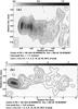 |
Fig. 8 Total-intensity images of 3C 345 obtained from the analysis of the GMVA data taken on May 2010. The full width at half maximum (FWHM) of the restoring beams are shown at the bottom-left corners: a) using uniform weighting of the visibilities (restoring beam with FWHM of 110 × 38 μas with a position angle of − 4.37 deg); and b) using natural weighting of the visibilities and tapering longest baselines (to enhance the sensitivity to extended structures; FWHM of 270 × 230 μas with a position angle of 62 deg). |
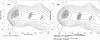 |
Fig. 9 Polarization images (superimposed on the total-intensity image) of 3C 345, when a) we average the D-terms estimated from the visibilities of a set of sources (3C 345, BLLAC, and 0716+714) and b) we use the D-terms directly estimated from the visibilities of 3C 345. The FWHM of the restoring beam is shown at the bottom-left corners. |
8. Summary
We have presented a well-defined calibration pipeline for global millimeter-VLBI (GMVA) observations. With this pipeline, it is possible to estimate all the instrumental effects in an optimal way, dealing with the particulars of the (typically complicated) schedules of global 3 mm VLBI observations and the inherent complications caused by the high observing frequency (86 GHz). All the scripts used in the pipeline are written in a generic way, hence can be easily executed and adapted to all the GMVA (and eventually non-GMVA) datasets. These scripts will indeed still be valid when new stations eventually join the GMVA in a near future.
Our scripts allow us to perform manual phase calibration (i.e., alignment of the phases among the different sub-bands) regardless of the subarraying conditions typically found in the data. The script also corrects for time-dependent phase and delay drifts between subbands, caused by variations in the electronics of the antenna receivers.
We have performed the GFF by optimizing the integration time of the fringes within the real coherence time of the visibilities. In the case of the GMVA, we have shown that integration times of up to several minutes maximize the S/N of the fringes, which indicates that there was only a moderate atmospheric degradation of the incoming phase at 86 GHz.
The visibility amplitudes are calibrated by fitting the temperature of the receivers of each antenna (and polarization) to the distribution of system temperatures over airmass. The opacity is then directly derived from the ambient and system temperatures for each antenna and time. In the cases of antennas where the atmospheric absorption is directly accounted for in the amplitude calibration, we can still refine the opacity correction with our approach.
For the polarization calibration, we have performed a manual phase calibration of the cross-polarization visibilities (i.e., we align the phases of the cross-polarization visibilities among the sub-bands) by imposing the same fringe rates in both polarizations for all the antennas and times. This calibration allows us to determine the leakage in the receivers (i.e., the D-terms) using the data of all subbands together, thus increasing the S/N of the gain solutions to be twice as large as those estimated from independent fits to the different subbands.
Our scripts also allow us to perform a Monte Carlo analysis to determine the effects of different D-term calibrations on the final full-polarization images. For the data reported here, a cut-off in the polarization images at the level of 50–60% of the intensity peak generates images that are typically very similar, regardless of the D-term calibration. The absolute position of the polarization features can also be affected by the D-term calibration, but this effect is no larger than the size of the synthesized beam.
As an example of our pipeline output, we show full-polarization images of source 3C 345, obtained from observations performed during the GMVA session of May 2010. The polarization images show a strong component on the north-east side of the source core, with a north-south electric vector position angle that rotates counter-clockwise along the jet (i.e., along the west direction). There are also two polarization components at about 0.1 mas and 0.2 mas from the core, for which the electric vector position angle is aligned with the direction of the jet and similar to the electric vector position angle observed at 43 GHz from VLBA observations taken a few days before our GMVA session.
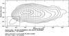 |
Fig. 10 VLBI image of the inner core region of 3C345 at 43 GHz (Jorstad et al., in prep.), observed on 19 May 2010. |
In upcoming GMVA sessions, we expect to be able to provide the end user with fully calibrated datasets, which will become available shortly after the data correlation.
Acknowledgments
The National Radio Astronomy Observatory is a facility of the National Science Foundation operated under cooperative agreement by Associated Universities, Inc. Based on observations with the 100-m telescope of the MPIfR (Max-Planck-Institut für Radioastronomie) at Effelsberg. Based on observations carried out with the IRAM Plateau de Bure Interferometer and the IRAM telescope at Pico Veleta. IRAM is supported by INSU/CNRS (France), MPG (Germany) and IGN (Spain).
References
- Attridge, J. M. 2001, ApJ, 553, L31 [NASA ADS] [CrossRef] [Google Scholar]
- Attridge, J. M., Wardle, J. F. C., Homan, D. C., & Phillips, R. B. 2005, ASPC, 340, 171 [NASA ADS] [Google Scholar]
- Baath, L. B., Rogers, A. E. E., Inoue, M., et al. 1992, A&A, 257, 31 [NASA ADS] [Google Scholar]
- Broderick, A. E., & Loeb, A. 2009, ApJ, 697, 1164 [NASA ADS] [CrossRef] [Google Scholar]
- Dodson, R. 2009 [arXiv:0910.1707] [Google Scholar]
- Gómez, J. L., Marscher, A. P., Alberdi, A., et al. 2002, VLBA Scientific Memo #30 [Google Scholar]
- Gómez, J. L., Roca-Sogorb, M., Agudo, I., et al. 2011, ApJ, 733, 11 [NASA ADS] [CrossRef] [Google Scholar]
- Homan, D. C., Lister, M. L., Aller, H. D., et al. 2009, ApJ, 696, 328 [NASA ADS] [CrossRef] [Google Scholar]
- Kettenis, M., van Langevelde, H. J., Reynolds, C., & Cotton, B. 2006, ASPC, 351, 497 [Google Scholar]
- Leppännen, K. J., Zensus, A. J., & Diamond, P. J. 1995, AJ, 110, 2479 [NASA ADS] [CrossRef] [Google Scholar]
- Marscher, A. P., Svetlana, G. J., John, P. M., et al. 2002, ApJ, 577, 85 [NASA ADS] [CrossRef] [Google Scholar]
- Martí-Vidal, I., & Marcaide, J. M. 2008, A&A, 480, 289 [NASA ADS] [CrossRef] [EDP Sciences] [Google Scholar]
- Mc Kinney, J. C., Tchekhovskoy, A., & Blandford, R. D. 2012, MNRAS, in press [arXiv:1201.4163] [Google Scholar]
- O’Sullivan, S. P., Gabuzda, D. C., & Gurvits, L. I. 2011, MNRAS, 415, 3049 [NASA ADS] [CrossRef] [Google Scholar]
- Penzias, A. A., & Burrus, C. A. 1973, ARA&A, 11, 51 [NASA ADS] [CrossRef] [Google Scholar]
- Rogers, A. E. E., Moffet, A. T., Backer, D. C., & Moran, J. M. 1984, Radio Sci., 19, 1552 [NASA ADS] [CrossRef] [Google Scholar]
- Rogers, A. E. E., Doeleman, S. S., & Moran, J. M. 1995, AJ, 109, 1391 [NASA ADS] [CrossRef] [Google Scholar]
- Shepherd, M. C., Pearson, T. J., & Taylor, G. B. 1994, BAAS, 26, 987 [NASA ADS] [Google Scholar]
- Schwab, F. R., & Cotton, W. D. 1983, AJ, 88, 688 [NASA ADS] [CrossRef] [Google Scholar]
- Tchekhovskoy, A., Narayan, R., & Mc Kinney, J. C. 2011, MNRAS, 418, L79 [NASA ADS] [CrossRef] [Google Scholar]
All Tables
All Figures
|
Fig. 1 Single-band phases (upper figures) and delays (lower figures) in the second subband of Fort Davis (left) and Plateau de Bure (right), referred to Los Alamos, for both circular polarizations. Times are given in day of the year (DOY). The gains are referred to the first subband in the LCP polarization. Solid lines are the interpolations applied to calibrate the data. Note that these plots show data for all sources. |
| In the text | |
|
Fig. 2 Fringe-rate spectra at the baselines of Effelsberg to Los Alamos (EF-LA, baseline of 7831 km) and Kitt Peak to Los Alamos (KP-LA, baseline of 752 km), for an observation of source 3C 273B with an integration time of four minutes. |
| In the text | |
|
Fig. 3 Multi-band delay between the antennas at Brewster and Los Alamos vs. time. Notice that data of all sources have been included in this plot. |
| In the text | |
|
Fig. 4 Left, delay differences between LCP and RCP at Los Alamos. Right, phase differences at the same station (referred to those in the subband at the lowest frequency, IF1). |
| In the text | |
|
Fig. 5 Left, system temperatures (Tsys) measured at Los Alamos vs. airmass. Straight lines are fits of linear models to the lower envelopes of the Tsys distributions. The receiver temperature is estimated as the extrapolation of the lower envelope to a null airmass. Right, zenith opacity (i.e., opacity multiplied by the sine of the antenna elevation) at Los Alamos vs. time, as estimated using Eq. (1). |
| In the text | |
|
Fig. 6 Distribution of the intensity peaks of the differential polarization images (see text) of source 3C 345, after dividing by the peak of the reference polarization image. |
| In the text | |
|
Fig. 7 a) Distribution of the shifts in the intensity peaks of all the polarization images obtained in our Monte Carlo D-term analysis. b) Same as Fig. 6, but taking into account the peak shifts before computing the differential polarization images. |
| In the text | |
|
Fig. 8 Total-intensity images of 3C 345 obtained from the analysis of the GMVA data taken on May 2010. The full width at half maximum (FWHM) of the restoring beams are shown at the bottom-left corners: a) using uniform weighting of the visibilities (restoring beam with FWHM of 110 × 38 μas with a position angle of − 4.37 deg); and b) using natural weighting of the visibilities and tapering longest baselines (to enhance the sensitivity to extended structures; FWHM of 270 × 230 μas with a position angle of 62 deg). |
| In the text | |
|
Fig. 9 Polarization images (superimposed on the total-intensity image) of 3C 345, when a) we average the D-terms estimated from the visibilities of a set of sources (3C 345, BLLAC, and 0716+714) and b) we use the D-terms directly estimated from the visibilities of 3C 345. The FWHM of the restoring beam is shown at the bottom-left corners. |
| In the text | |
|
Fig. 10 VLBI image of the inner core region of 3C345 at 43 GHz (Jorstad et al., in prep.), observed on 19 May 2010. |
| In the text | |
Current usage metrics show cumulative count of Article Views (full-text article views including HTML views, PDF and ePub downloads, according to the available data) and Abstracts Views on Vision4Press platform.
Data correspond to usage on the plateform after 2015. The current usage metrics is available 48-96 hours after online publication and is updated daily on week days.
Initial download of the metrics may take a while.