| Issue |
A&A
Volume 542, June 2012
|
|
|---|---|---|
| Article Number | A104 | |
| Number of page(s) | 7 | |
| Section | Stellar atmospheres | |
| DOI | https://doi.org/10.1051/0004-6361/201118297 | |
| Published online | 15 June 2012 | |
Chemical composition of semi-regular variable giants. III.⋆,⋆⋆
1 Department of Astronomy and Astronomical Observatory, Odessa National University, T.G. Shevchenko Park, 65014 Odessa;
Isaac Newton Institute of Chile, Odessa Branch, Ukraine
e-mail: britvavskiy@gmail.com; scan@deneb1.odessa.ua; serkor@skyline.od.ua
2 GEPI, Observatoire de Paris-Meudon, 92125 Meudon Cedex, France
3 Tavrian National University, Yaltinskaya 4, 330000 Simferopol, Crimea, Ukraine
4 WIYN Observatory, 950 N Cherry Ave, Tucson, AZ 85719, USA
e-mail: rpm2112@gmail.com
Received: 19 October 2011
Accepted: 20 March 2012
Aims. We derive the stellar atmosphere parameters and chemical element abundances of four stars classified as semi-regular variables of type “d” (SRd). These stars should presumably belong to the Galactic halo population.
Methods. Elemental abundances are derived by applying both local thermodynamical equilibrium and non-local thermodynamical equilibrium analyses to high resolution (R ≈ 80 000) spectra obtained with the CFHT ESPaDOnS spectrograph. We determine the abundances of 27 chemical elements in VW Dra, FT Cnc, VV LMi, and MQ Hya.
Results. The stars of our present program have a chemical composition that is inconsistent with their presumable status as metal-deficient halo giants. All studied SRd giants have relative-to-solar elemental abundances that are typical of the thick/thin Galactic disk stars. We find that all objects of this class for which spectroscopic follow up analyses have been completed show a dichotomy in the amplitudes of their photometric variations. Specifically, the disk objects have small amplitudes, while halo SRd stars have much larger amplitudes, which indicates that amplitude is obviously related to the metallicity of the star.
Key words: stars: abundances / stars: variables: general / stars: late-type / stars: fundamental parameters
Based on observations obtained at the Canada-France-Hawaii Telescope (CFHT), which is operated by the National Research Council of Canada, the Institut National des Sciences de l’Univers of the Centre National de la Recherche Scientifique of France, and the University of Hawaii.
Figures 2 and 3 are available in electronic form at http://www.aanda.org
© ESO, 2012
1. Introduction
This article continues a series of papers devoted to the spectroscopic investigation of SRd variable stars (semi-regular yellow giants). Our main objective is to find a definitive answer to the following question: do the stars classified as SRd have the physical and chemical characteristics typically found only for the halo stellar population? In the past, the SRd giants were considered as members of the stellar population II (Dawson et al. 1982; Wahlgren 1993). The kinematics of some of these stars are, however, consistent with a halo origin. For the majority of SRd stars, however, the relevant kinematical data are unavailable in the literature.
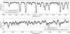 |
Fig. 1 Fragments of the VV LMi synthetic spectrum superimposed on its observed spectrum. |
Several abundance analyses of SRd stars have been performed (Andrievsky et al. 1985; Giridhar et al. 1998, 1999, 2000; Andrievsky et al. 2007a – Paper I). They have measured low relative-to-solar abundances of elements in these stars, which is typically a signature of halo/thick disk objects ([Fe/H] ≈ from –1.0 to –2.0). Nevertheless, the results of our most recent study (Britavskiy et al. 2010a – Paper II) indicated that the situation for SRd stars is rather complicated. All the stars investigated in that paper (V463 Her, V894 Her, CW CVn, and MS Hya) appear to have a chemical composition that does not agree with their presumable status as halo giants.
On the contrary, these giants have the relative-to-solar elemental abundances typical of the thick/thin Galactic disk stars (see Bensby et al. 2010, for the abundances of the disk stars). Thus, one can suppose that the SRd class comprises stars of both the halo and disk population objects. However, only a small number of these SRd stars have been investigated so far: only 21 of the 220 SRd stars known listed in the General Catalogue of Variable Stars (GCVS), have been studied by means of high-resolution spectroscopy, i.e. about 10%. We believe that it is necessary to increase the statistics to evaluate the relative number of SRd stars belonging to the halo and disk populations.
In this article, we present our measurements of the elemental abundances derived in VW Dra, FT Cnc, VV LMi, and MQ Hya. This was done for the first time for these stars (only VW Dra had previously been analyzed by Andrievsky et al. 1985, but using photographic plate material).
2. Observations
For our observations with the Canada-France-Hawaii 3.6-m telescope, we selected several SRd stars listed in GCVS. The observations were carried out over three nights in 2005 with the fiber-fed ESPaDOnS spectrograph equipped with a EEV 2000 × 4500 CCD camera (binned 1 × 1). The resolving power provided by this combination was about 80 000 and the spectral range extended from 3700 Å to 10 500 Å. The list of the stars and some of their characteristics are given in Table 1. For all the studied spectra, the signal-to-noise ratio (S/N) within the observed spectral fragments is higher than 100. The spectra were first processed by the CFHT ESPaDOnS reduction pipeline and then extracted using standard IRAF procedures (subtraction of dark, division by the flat fields, wavelength calibration, etc.). Additional analysis of the spectra (continuum placement, equivalent width measurements, spectra fragment extraction) was performed using the DECH20 code (Galazutdinov 1992). Correct continuum placement in the spectra of the cool stars is always problematic, and to some extent, the corresponding choice is subjective. To minimize the subjectivity, we applied a synthetic spectrum technique in order to find the real position of the continuum in the spectra of our cool program stars. The line list needed for the synthetic spectrum generation was taken from the VALD’s database1. This atomic line list was also supplemented with a molecular line list2. As an example, in Fig. 1 we show two fragments of the VV LMi synthetic spectrum generated with Tsymbal’s (1996) LTE code, and then superimposed on the observed spectrum of this star.
Characteristics of the program stars.
3. Analysis and results
The list of unblended or weakly blended lines possibly present was selected from the VALD database. For all the lines studied, this database lists the excitation potentials, oscillator strengths, and broadening parameters. Our spectroscopic analysis was based on LTE Kurucz atmosphere models (Kurucz 1992). The equivalent widths of the spectral lines selected for our analysis were measured using a Gaussian approximation. In all the spectra of our program stars, the absorption lines are narrow and symmetric, hence the equivalent widths of the lines were measured with high accuracy. An Arcturus spectrum (see Hinkle et al. 2000) was selected as an appropriate example to verify our analysis technique, since this is a well – investigated star and its atmosphere parameters are comparable to those of our program stars (Fulbright et al. 2007). In Tables 3 and 4, we give the results of the abundance analysis and a comparison with the data published by Fulbright et al. (2007).
3.1. Fundamental parameters
The effective temperature Teff for each star studied here was estimated using the line depth ratios. The line-depth ratio method, which is based on sensitive temperature indicators, was developed for giant stars by Kovtyukh et al. (2006). The method is independent of the interstellar reddening, and only marginally dependent on individual characteristics of the stars, such as rotation, microturbulence, and metallicity. The mean error in the Teff determination is no larger than 100–150 K. To verify the results of the temperature determination, we applied the standard procedure of avoiding any dependence of the iron abundance derived from the Fe i lines on their excitation potentials (Fig. 2).
We also applied a traditional method of effective temperature determination based on the use of colors. For our program stars, these colors were selected from SIMBAD. With calibrations published by Alonso et al. (1999) for the giant stars, we obtained the results that are gathered in Table 2. The expected accuracy of these determinations is not very high (about ± 250 K), but we can see that our effective temperatures based on the line depth ratios are in satisfactory agreement with photometric temperature estimates.
Comparison of the program-star effective temperatures determined using different methods.
To evaluate the microturbulent velocity (Vt) in the atmospheres of our program stars, we used a commonly used method based on the lack of a relation between the iron abundance produced by individual Fe i lines and their measured equivalent widths. Results are shown in Fig. 3.
The surface gravity of each program star was derived by maintaining the ionization balance of the iron abundance produced by both Fe i and Fe ii lines. The stellar atmosphere parameters of our program stars are given in Table 1.
3.2. Abundances
Since we used the VALD compilation of oscillator strengths, we eliminated possible random errors in the derived abundances by comparing the stellar elemental abundances with the solar values, which were determined with the same log gf values, the solar atmosphere model from the Kurucz’s grid, and microturbulent velocity of 1.3 km s-1. Our solar abundances were derived using the Kurucz Solar Flux Atlas (Kurucz et al. 1984). Since the Sun has at present the most reliably determined chemical abundances, this allows us to check the adopted atomic line list and exclude from the analysis the VALD lines that lead to significant deviations from the mean abundance results. We also note that in our analysis we used only the lines common to both the solar and program star spectra. Taking this into account, we therefore consider approach as the most grounded way to use the Sun as a reference star, despite the obvious difference between the effective temperatures of the Sun and our program stars. Nevertheless, we also checked our input atomic data using the Arcturus spectrum, as mentioned before in this section. The abundance results for the Sun and our program stars are presented in the next section.
To verify the accuracy of the abundances derived from our equivalent width analysis, we applied a synthetic spectrum technique (Tsymbal 1996, LTE code) to take into account the possible blending of some lines and continuum level distortion caused by molecular bands. This check was absolutely necessary for the three cooler stars of our sample, whose spectra display evidence of many molecular features.
It is also necessary to note that only a few Ti ii and Fe ii lines can be found in the spectra of these cool giants. These lines are important for determining the gravity. Therefore, we checked the sensitivity of the gravity determination by modeling the wings of the strong lines of the ionized calcium triplet. Our results are shown in Fig. 4 for three stars of our sample, as well as for Arcturus, for which we know the atmosphere model parameters with great accuracy.
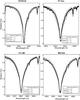 |
Fig. 4 LTE Ca i line profiles fitted to the observed spectrum for Arcturus and three cooler program stars. Relative flux = Fλ/Fc. Note that in some cases there is no possibility of reproducing the very central part of the investigated line. |
The abundances of elements such as O, Na, Mg, Al, S, K, Ca, and Ba were found using the NLTE spectral synthesis based on the modified version of MULTI code (see Carlsson 1986, for the MULTI description; and Korotin et al. 1999a,b; Korotin & Mishenina 1999; Mishenina et al. 2000, 2004; Andrievsky et al. 2001, 2007b, 2008, 2009, 2010; Korotin 2009, and references therein, for the description of the code modification and applied atomic models). When necessary, the NLTE code was combined with an LTE synthetic spectrum in order to take into account the blending of the lines treated in NLTE with lines of other species. For the other chemical elements investigated, the abundances were derived with the help of the Kurucz LTE WIDTH9 code.
Table 5 lists the relative-to-solar abundances in the stars of our sample. Graphically, the distribution of the chemical elements in the studied stars is shown in Fig. 5.
Relative-to-solar elemental abundances in our program stars.
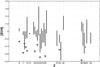 |
Fig. 5 Abundance distribution (the vertical segment for each element includes the spread of abundances for our four program stars), and lower limits to the corresponding elemental abundances in the thick disk stars ∇ (Bensby et al. 2010). Z is the atomic number. Abundance derived only in one of the program star is shown by a dot. |
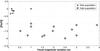 |
Fig. 6 Comparison of the ranges of visual magnitude variation for the halo and disk population objects. |
4. Discussion and conclusion
Our results presented in Table 5 show that all investigated stars have elemental abundances that are atypical of the halo population. For some elements, the scatter from star to star is rather large (e.g. for Y and La), but the lowest abundances of the vast majority of the investigated elements in our sample are no lower than those seen in the stars belonging to the thick disk (according to Bensby et al. 2010, the relative-to-solar iron abundance [Fe/H] of the thick disk stars is within the range from about zero to –1 dex). From the elements in common with the investigation of Bensby et al. (2010) in the thick disk stars (see their Fig. 10) and us, only two elements have surprising differences in their abundances. In Fig. 5, we compare the elemental abundances of the four stars in the present study with lower limits to the thick disk stellar abundances.
Among the 21 stars of the SRd class studied up to now (see references in the Introduction), 12 show the elemental abundances that allow one to classify them as halo population objects, while the other stars apparently belong to the thick and thin Galactic disks. We note that both groups of SRd stars clearly have differences in the amplitudes of their visual magnitude variation. The halo members with significantly lower metallicities have much larger amplitudes, while the amplitudes of the stars with [Fe/H] greater than –1 are much smaller (Fig. 6). However, the relation between the amplitude of luminosity variation and the metallicity of the star, and the mechanism behind this amplitude modulation remains unclear.
Thus, we can conclude that we have obtained evidence that the SRd class is chemically inhomogeneous. This class comprises both the halo and disk population objects, which nevertheless can manifest similar photometric semi-regular variabilities.
Online material
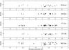 |
Fig. 2 Relative-to-solar iron abundance from derived Fe i lines versus excitation potential for Arcturus and for SRd stars of our program. As is the convention in spectroscopic literature, hereafter we denote the relative-to-solar abundance of a certain element as [El/H] = log ϵ(El) – log ϵ(El)⊙. |
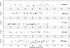 |
Fig. 3 Relative-to-solar iron abundances derived from the Fe i lines versus the equivalent widths of Arcturus and SRd stars in our program. |
R. L. Kurucz, http://kurucz.harvard.edu/molecules.htm
Acknowledgments
S.M.A. and S.A.K. kindly acknowledges the partial support from SCOPES grant No. IZ73Z0-128180/1. We also acknowledge the CFHT support staff for their help during the observations. This research has made use of the SIMBAD database, operated at CDS, Strasbourg, France. We thank an anonymous referee for valuable comments that we believe improved this paper. We also sincerely thank Dr. Ralf Napiwotzki for helpful comments.
References
- Alonso, A., Arribas, S., & Martinez-Roger, C. 1999, A&AS, 140, 261 [NASA ADS] [CrossRef] [EDP Sciences] [Google Scholar]
- Andrievsky, S. M., Makarenko, E. N., & Fenina, Z. N. 1985, PrKFi, 20, 60 [NASA ADS] [Google Scholar]
- Andrievsky, S. M., Kovtyukh, V. V., Korotin, S. A., Spite, M., & Spite, F. 2001, A&A, 367, 605 [NASA ADS] [CrossRef] [EDP Sciences] [Google Scholar]
- Andrievsky, S. M., Korotin, S. A., & Martin, P. 2007a, A&A, 464, 709 (Paper I) [NASA ADS] [CrossRef] [EDP Sciences] [Google Scholar]
- Andrievsky, S. M., Spite, M., Korotin, S. A., et al. 2007b, A&A, 464, 1081 [NASA ADS] [CrossRef] [EDP Sciences] [Google Scholar]
- Andrievsky, S. M., Spite, M., Korotin, S. A., et al. 2008, A&A, 481, 481 [NASA ADS] [CrossRef] [EDP Sciences] [Google Scholar]
- Andrievsky, S. M., Spite, M., Korotin, S. A., et al. 2009, A&A, 494, 1083 [NASA ADS] [CrossRef] [EDP Sciences] [Google Scholar]
- Andrievsky, S. M., Spite, M., Korotin, S. A., et al. 2010, A&A, 509, A88 [NASA ADS] [CrossRef] [EDP Sciences] [Google Scholar]
- Bensby, T., Feltzing, S., Johnson, J. A., et al. 2010, A&A, 512, A41 [NASA ADS] [CrossRef] [EDP Sciences] [Google Scholar]
- Britavskiy, N. E., Andrievsky, S. M., Korotin, S. A., & Martin, P. 2010a, A&A, 519, A74 (Paper II) [NASA ADS] [CrossRef] [EDP Sciences] [Google Scholar]
- Carlsson, M. 1986, Uppsala Astron. Obs. Rep., 33 [Google Scholar]
- Dawson, D. W., & Patterson, C. R. 1982, PASP, 94, 574 [NASA ADS] [CrossRef] [Google Scholar]
- Edvardsson, B., Andersen, J., Gustafsson, B., et al. 1993, A&A, 275, 101 [NASA ADS] [Google Scholar]
- Fulbright, J. P., McWilliam, A., & Rich, R. M. 2007, ApJ, 661, 1152 [NASA ADS] [CrossRef] [Google Scholar]
- Galazutdinov, G. A. 1992, Preprint SAO RAS, No. 92 [Google Scholar]
- Giridhar, S., Lambert, D., & Gonzalez, G. 1998, PASP, 110, 671 [NASA ADS] [CrossRef] [Google Scholar]
- Giridhar, S., Lambert, D., & Gonzalez, G. 1999, PASP, 111, 1269 [NASA ADS] [CrossRef] [Google Scholar]
- Giridhar, S., Lambert, D., & Gonzalez, G. 2000, PASP, 112, 1559 [NASA ADS] [CrossRef] [Google Scholar]
- Hinkle, K., Wallace, L., Valenti, J., & Harmer, D. 2000, Visible and Near Infrared Atlas of the Arcturus Spectrum 3727-9300 (San Francisco: ASP) [Google Scholar]
- Korotin, S. A. 2009, Astron. Rep., 53, 651 [NASA ADS] [CrossRef] [Google Scholar]
- Korotin, S. A., & Mishenina, T. V. 1999, Astron. Rep., 43, 533 [NASA ADS] [Google Scholar]
- Korotin, S. A., Andrievsky, S. M., & Luck, R. E. 1999a, A&A, 351, 168 [NASA ADS] [Google Scholar]
- Korotin, S. A., Andrievsky, S. M., & Kostynchuk, L. Yu. 1999b, Ap&SS, 260, 531 [NASA ADS] [CrossRef] [Google Scholar]
- Kovtyukh, V. V., Mishenina, T. V., Gorbaneva, T. I., et al. 2006, Astron. Rep., 50, 134 [Google Scholar]
- Kurucz, R. L. 1992, RMxAA, 23, 45 [Google Scholar]
- Kurucz, R. L., Furenlid, I., Brault, J., & Testerman, L. 1984, Solar flux atlas from 296 to 1300 nm (New Mexico: National Solar Observatory) [Google Scholar]
- Peterson, R. C., Dalle Ore, C. M., & Kurucz, R. L. 1993, ApJ, 404, 333 [NASA ADS] [CrossRef] [Google Scholar]
- Mishenina, T. V., Korotin, S. A., Klochkova, V. G., & Panchuk, V. E. 2000, A&A, 353, 978 [NASA ADS] [Google Scholar]
- Mishenina, T. V., Soubiran, C., Kovtyukh, V. V., & Korotin, S. A. 2004, A&A, 418, 551 [NASA ADS] [CrossRef] [EDP Sciences] [Google Scholar]
- Tsymbal, V. V. 1996, Model Atmospheres and Spectrum Synthesis, ed. S. J. Adelman, F. Kupka, & W. W. Weiss (San Francisco), ASP Conf. Ser., 108 [Google Scholar]
- Wahlgren, G. M. 1993, ASPC, 45 [Google Scholar]
All Tables
Comparison of the program-star effective temperatures determined using different methods.
All Figures
|
Fig. 1 Fragments of the VV LMi synthetic spectrum superimposed on its observed spectrum. |
| In the text | |
|
Fig. 4 LTE Ca i line profiles fitted to the observed spectrum for Arcturus and three cooler program stars. Relative flux = Fλ/Fc. Note that in some cases there is no possibility of reproducing the very central part of the investigated line. |
| In the text | |
|
Fig. 5 Abundance distribution (the vertical segment for each element includes the spread of abundances for our four program stars), and lower limits to the corresponding elemental abundances in the thick disk stars ∇ (Bensby et al. 2010). Z is the atomic number. Abundance derived only in one of the program star is shown by a dot. |
| In the text | |
|
Fig. 6 Comparison of the ranges of visual magnitude variation for the halo and disk population objects. |
| In the text | |
|
Fig. 2 Relative-to-solar iron abundance from derived Fe i lines versus excitation potential for Arcturus and for SRd stars of our program. As is the convention in spectroscopic literature, hereafter we denote the relative-to-solar abundance of a certain element as [El/H] = log ϵ(El) – log ϵ(El)⊙. |
| In the text | |
|
Fig. 3 Relative-to-solar iron abundances derived from the Fe i lines versus the equivalent widths of Arcturus and SRd stars in our program. |
| In the text | |
Current usage metrics show cumulative count of Article Views (full-text article views including HTML views, PDF and ePub downloads, according to the available data) and Abstracts Views on Vision4Press platform.
Data correspond to usage on the plateform after 2015. The current usage metrics is available 48-96 hours after online publication and is updated daily on week days.
Initial download of the metrics may take a while.