© ESO, 2012

1. Introduction

A global structure of the pulsar magnetosphere is the key question to answer for understanding the energy outflow to the exterior. Likely, the magnetospheres consist of electron-positron plasma with some amounts of ions. This plasma can affect the radiation produced in the inner region of the magnetosphere or at the stellar surface. Therefore, understanding the properties of a magnetosphere is of crucial importance for the interpretation of observations. In recent years, some progress has been achieved in theoretical models of the pulsar magnetosphere (see, e.g., Goodwin et al. 2004; Contopoulos et al. 1999; Komissarov 2006). Apart from a quasi-static structure, however, various non-stationary phenomena (such as waves, instabilities, etc.) can play an important role. They also may affect the radiation but, perhaps, idealised quasi-static magnetospheric models cannot be valid in the presence of physical instabilities. For example, the electrostatic oscillations with a low frequency have been considered recently by Mofiz et al. (2012), who found that the thermal and magnetic pressures can generate oscillations that propagate near the equator. These low-frequency electromagnetic waves are of central importance for understanding the underlying processes in the formation of the radio spectrum (see, e.g., Melrose 1996, and reference therein).

Instabilities of magnetohydrodynamic modes can also occur in the pulsar magnetosphere. For typical values of the magnetic field, the electromagnetic energy density is much greater than the kinetic and thermal energy density. This suggests that for much of the magnetosphere, the force-free condition is a good approximation for determining the magnetic field. Magnetohydrodynamic (MHD) processes under this condition are poorly studied but they might be very particular. One of the MHD phenomena that can occur in the pulsar magnetosphere is the so-called diocotron instability, which is the non-neutral plasma analog of the Kelvin-Helmholtz instability. This instability has been studied extensively in the context of laboratory plasma devices (see, e.g., Levy 1965; Davidson 1990; Davidson & Felice 1998). The existence around pulsars of a differentially rotating equatorial disc with non-vanishing charge density could trigger a shearing instability of diocotron modes (Petri et al. 2002). In the non-linear regime, the diocotron instability can cause diffusion of the charged particles across the magnetic field lines outwards (Petri et al. 2003). The role of a diocotron instability in causing drifting subpulses in radio pulsar emission has been considered by Fung et al. (2006). Note that the diocotron modes should be substantially suppressed in a neighbourhood of the light cylinder where relativistic effects become important (Petri 2007).

Recently, one more mode of magnetospheric oscillations has been considered by Urpin (2011). This mode is closely related to the Alfvenénic waves of the standard magnetohydrodynamics modified by the force-free condition and non-vanishing electric charge density. Like Alfvén waves, the magnetospheric waves of a small amplitude are transverse (plasma motions are perpendicular to the wavevector). The magnetospheric waves can be unstable because there is a number of destabilising factors in the magnetosphere (differential rotation, electric currents, non-zero charge density, etc.). The electric current usually provides a destabilising effect that leads to the so-called Tayler instability (see, e.g., Tayler 1973a,b). This instability is well studied in both laboratory and stellar conditions. It arises on the Alfvén time scale and is particularly efficient if the strengths of the toroidal and poloidal field components differ substantially (see, e.g., Bonanno & Urpin 2008a,b). This condition can be fulfilled in many magnetospheric models (see, e.g., Contopoulos et al. 1999).

Various models of the magnetosphere predict that rotation should be differential (e.g., Mestel & Shibata 1994; Contopoulos et al. 1999). It is known that differential rotation in combination with the magnetic field leads to the magnetorotational instability (Velikhov 1959; Balbus & Hawley 1991). This instability may occur even in a very strong magnetic field (Urpin & Rüdiger 2005). However, the instability in the pulsar magnetosphere can differ qualitatively from the standard magnetorotational instability because of non-vanishing charge density and the force-free condition. In this paper, we consider the instability in the pulsar magnetosphere caused by differential rotation.

2. Basic equations

Despite uncertainties in estimates of many parameters, plasma in the pulsar magnetosphere is likely collisional and the Coulomb mean free path of particles is shorter than the characteristic length scale. Therefore, the MHD description can be applied to such plasma. The partial MHD momentum equations for the electrons and positrons can be obtained by multiplying the Boltzmann kinetic equation by the velocity and integrating over it. Assuming that plasma is non-relativistic, the momentum equation for particles of the sort α (α = e,p) reads $\begin{array}{ccc}{\mathit{m}}_{\mathit{\alpha }}{\mathit{n}}_{\mathit{\alpha }}\left[\dot{{V}}\mathit{\alpha }\mathrm{+}\mathrm{(}{{V}}_{\mathit{\alpha }}\mathrm{·}\mathrm{\nabla }\mathrm{)}{{V}}_{\mathit{\alpha }}\right]\mathrm{=}\mathrm{-}\mathrm{\nabla }{\mathit{p}}_{\mathit{\alpha }}\mathrm{+}{\mathit{n}}_{\mathit{\alpha }}{F}\mathit{\alpha }& & \\ \mathrm{+}{\mathit{e}}_{\mathit{\alpha }}{\mathit{n}}_{\mathit{\alpha }}\left({E}\mathrm{+}\frac{{{V}}_{\mathit{\alpha }}}{\mathit{c}}\mathrm{\times }{B}\right)\mathrm{+}{{R}}_{\mathit{\alpha }}& & \end{array}$(1)(see, e.g., Braginskii 1965, where the general plasma formalism is developed); the dot denotes the partial time derivative. Here, V_α is the mean velocity of particles α, n_α and p_α are their number density and pressure, respectively, F_α is an external force acting on the particles α (in our case F_α is the gravitational force), E and B are the electric and magnetic fields, respectively: R_α is the internal friction force caused by collisions of the particles α with other sorts of particles. Since R_α is the internal force, the sum of R_α over α is zero in accordance with Newton’s third law. Hence, we have in the electron-positron plasma R_e =  −R_p.

A calculation of R_α is a very complicated problem of plasma physics but we will obtain it using simple physical arguments. Generally, R_α is proportional to the difference of partial velocities of particles (V_e − V_p) and to the temperature gradient (see, e.g., Braginskii 1965). We will neglect thermal diffusion in R_α because it is usually small in astrophysical conditions and take into account only friction caused by a difference in the partial velocities. Then, ${{R}}_{\mathrm{e}}\mathrm{=}\mathrm{-}\frac{{\mathit{m}}_{\mathrm{e}}{\mathit{n}}_{\mathrm{e}}}{{\mathit{\tau }}_{\mathrm{e}}}\mathrm{(}{{V}}_{\mathrm{e}}\mathrm{-}{{V}}_{\mathrm{p}}\mathrm{)}\mathit{,}$(2)where τ_e is the relaxation time of electrons. Note that this simple expression for R_e is often used even in a laboratory plasma (Braginskii 1965) and yields qualitatively correct results. We assume that accuracy of Eq. (2) is sufficient in the pulsar magnetosphere as well.

In the electron-positron plasma, both sorts of particles have a small mass and the inertial force can be neglected in Eq. (1). The gravitation force is also weak because of a small mass, and the gas pressure is much smaller than the magnetic pressure. Hence, both these forces can be neglected in Eq. (1) as well. Then, we have ${\mathit{e}}_{\mathit{\alpha }}{\mathit{n}}_{\mathit{\alpha }}\left({E}\mathrm{+}\frac{{{V}}_{\mathit{\alpha }}}{\mathit{c}}\mathrm{\times }{B}\right)\mathrm{+}{{R}}_{\mathit{\alpha }}\mathrm{=}\mathrm{0.}$(3)It is more convenient to use linear combinations of Eq. (3) rather than to solve partial equations. Let us define the hydrodynamic velocity and electric current as ${V}\mathrm{=}\frac{\mathrm{1}}{\mathit{n}}\mathrm{(}{\mathit{n}}_{\mathrm{e}}{{V}}_{\mathrm{e}}\mathrm{+}{\mathit{n}}_{\mathrm{p}}{{V}}_{\mathrm{p}}\mathrm{)}\mathit{,}{j}\mathrm{=}\mathit{e}\mathrm{(}{\mathit{n}}_{\mathrm{p}}{{V}}_{\mathrm{p}}\mathrm{-}{\mathit{n}}_{\mathrm{e}}{{V}}_{\mathrm{e}}\mathrm{)}\mathit{,}$(4)where n = n_e + n_p. Then, the velocities of the electrons and positrons are ${{V}}_{\mathrm{e}}\mathrm{=}\frac{\mathrm{1}}{\mathrm{2}{\mathit{n}}_{\mathrm{e}}}\left(\mathit{n}{V}\mathrm{-}\frac{{j}}{\mathit{e}}\right)\mathit{,}{{V}}_{\mathrm{p}}\mathrm{=}\frac{\mathrm{1}}{\mathrm{2}{\mathit{n}}_{\mathrm{p}}}\left(\mathit{n}{V}\mathrm{+}\frac{{j}}{\mathit{e}}\right)\mathrm{·}$(5)If n is much greater than the charge number density |n_p − n_e|, we have V ≫ j/en. However, this inequality cannot be valid if |n_p − n_e| ~ n. In the general case, the sum of electron and positron Eqs. (3) yields the equation of hydrostatic equilibrium 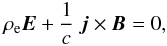$\begin{array}{ccc}{\mathit{\rho }}_{\mathrm{e}}{E}\mathrm{+}\frac{\mathrm{1}}{\mathit{c}}{j}\mathrm{\times }{B}\mathrm{=}\mathrm{0}\mathit{,}& & \end{array}$(6)where ρ_e = e(n_p − n_e) = eδn is the charge density. Taking the difference of Eq. (3) for electrons and positrons, we obtain 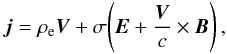${j}\mathrm{=}{\mathit{\rho }}_{\mathrm{e}}{V}\mathrm{+}\mathit{\sigma }\left({E}\mathrm{+}\frac{{V}}{\mathit{c}}\mathrm{\times }{B}\right)\mathit{,}$(7)where σ = e²n_pτ_e/m_e is the conductivity of plasma.

Equations (6) and (7) can be written as 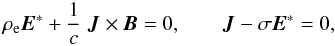${\mathit{\rho }}_{\mathrm{e}}{{E}}^{\mathrm{\ast }}\mathrm{+}\frac{\mathrm{1}}{\mathit{c}}{J}\mathrm{\times }{B}\mathrm{=}\mathrm{0}\mathit{,}{J}\mathrm{-}\mathit{\sigma }{{E}}^{\mathrm{\ast }}\mathrm{=}\mathrm{0}\mathit{,}$(8)where ${{E}}^{\mathrm{\ast }}\mathrm{=}{E}\mathrm{+}\frac{{V}}{\mathit{c}}\mathrm{\times }{B}\mathit{,}{J}\mathrm{=}{j}\mathrm{-}{\mathit{\rho }}_{\mathrm{e}}{V}\mathit{.}$(9)Eliminating E^∗ from Eq. (8) in favour of J, we have 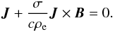${J}\mathrm{+}\frac{\mathit{\sigma }}{\mathit{c}{\mathit{\rho }}_{\mathrm{e}}}{J}\mathrm{\times }{B}\mathrm{=}\mathrm{0.}$(10)It follows immediately from this equation that J_∥ = 0. Calculating the cross production of Eq. (10) and B, we obtain J_⊥ = 0 as well. Then, second Eq. (8) yields E^∗ = 0. Hence, Eqs. (6)–(7) are equivalent to the conditions 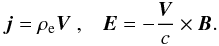${j}\mathrm{=}{\mathit{\rho }}_{\mathrm{e}}{V}\mathit{,}{E}\mathrm{=}\mathrm{-}\frac{{V}}{\mathit{c}}\mathrm{\times }{B}\mathit{.}$(11)This implies that the force-free condition in combination with Ohm’s law (Eq. (7)) is equivalent to the condition of the frozen-in magnetic field and the presence of only advective currents. Or, in other words, the force-free condition and Ohm’s law are compatible only if the electric current is poorly advective and the magnetic field is frozen-in. Note that this statement is valid at any relation between the electron and positron number densities.

3. Instability in the pulsar magnetosphere

The set of MHD equations complemented by the Maxwell equations reads in the force-free pulsar magnetosphere 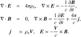$\begin{array}{ccc}\mathrm{\nabla }\mathrm{·}{E}& \mathrm{=}& \mathrm{4}\mathit{\pi }{\mathit{\rho }}_{\mathrm{e}}\mathit{,}\mathrm{\nabla }\mathrm{\times }{E}\mathrm{=}\mathrm{-}\frac{\mathrm{1}}{\mathit{c}}\frac{\mathit{\partial }{B}}{\mathit{\partial t}}\mathit{,}\\ \mathrm{\nabla }\mathrm{·}{B}& \mathrm{=}& \mathrm{0}\mathit{,}\mathrm{\nabla }\mathrm{\times }{B}\mathrm{=}\frac{\mathrm{1}}{\mathit{c}}\frac{\mathit{\partial }{E}}{\mathit{\partial t}}\mathrm{+}\frac{\mathrm{4}\mathit{\pi }}{\mathit{c}}{j}\mathit{,}\\ {j}& \mathrm{\approx }& {\mathit{\rho }}_{\mathrm{e}}{V}\mathit{,}{E}\mathrm{\approx }\mathrm{-}\frac{{V}}{\mathit{c}}\mathrm{\times }{B}\mathit{.}\end{array}$(12)Note one important property of steady state magnetospheres (∂/∂t = 0). Such magnetospheres can exist only if the hydrodynamic velocity is non-vanishing, V ≠ 0. Indeed, let us assume that V = 0. Then, we have from Eqs. (12) that j and E are equal to zero. If the electric field is zero then ρ_e is also vanishing. Since j = 0 the magnetic field has a vacuum structure (∇·B = 0, ∇ × B = 0), which means that the magnetosphere does not exist at all. The conclusion that there should exist hydrodynamic flows in the magnetosphere is the intrinsic property of the equations of the force-free magnetohydrodynamics and is valid at any relation between the electron and positron number densities.

The MHD processes governed by Eqs. (12) are very particular, which point can be illustrated by considering a linear instability. We assune that the electric and magnetic fields are equal to E₀ and B₀ in the unperturbed magnetosphere. The unperturbed charge density and velocity are ρ_e0 and V₀, respectively. For the sake of simplicity, we assume that motions in the magnetosphere are non-relativistic, V₀ ≪ c. Linearising Eqs. (12), we can obtain the set of equations that describes the behaviour of modes with a low amplitude. Small perturbations will be indicated by subscript 1. For the sake of simplicity, we treat instability of an axisymmetric magnetosphere with respect to axisymmetric perturbations. We consider perturbations with a short wavelength and space-time dependence  ∝ exp(iωt − ik·r) where ω and k are the frequency and wave vector, respectively; the wave vector k has no ϕ-component. A short wavelength approximation applies if the wavelength of perturbations, λ = 2π/k, is short compared to the characteristic length scale of the magnetosphere, L. Note that, generally, the instability criteria for short wavelength perturbations can differ from those for global modes with the lengthscale comparable to L. Instability of global modes is usually sensitive to details of the global magnetospheric structure and boundary conditions, which are quite uncertain in the pulsar magnetosphere. In contrast, the instability of short wavelength perturbations is entirely determined by local characteristics of the magnetosphere, which are less uncertain. Note also that the boundary conditions and instability of global modes can seriously modify a non-linear development of short wavelength perturbations, particularly if the global modes grow faster than the short wavelength modes. However, in this paper we consider only a linear stage of instability.

As explained above, instability can occur because of either differential rotation or electric currents. The structure of a pulsar magnetosphere and its magnetic topology is quite uncertain even in the axisymmetric model. Therefore, we consider in this paper only instability caused by differential rotation and neglect effects associated to electric currents. We will show that instability caused by differential rotation can arise at any magnetic geometry.

Substituting the frozen-in condition E =  −V × B/c into the equation c∇ × E =  −∂B/∂t (Eq. (12)) and linearising the obtained induction equation, we have $\mathrm{i}\mathit{\omega }{{B}}_{\mathrm{1}}\mathrm{=}\mathrm{\nabla }\mathrm{\times }\mathrm{(}{{V}}_{\mathrm{1}}\mathrm{\times }{{B}}_{\mathrm{0}}\mathrm{+}{{V}}_{\mathrm{0}}\mathrm{\times }{{B}}_{\mathrm{1}}\mathrm{)}\mathit{.}$(13)If the unperturbed velocity is caused mainly by rotation, V₀ = sΩe_ϕ where s is the cylindrical radius and e_ϕ the unit vector in the ϕ-direction, then $\mathrm{i}\mathit{\omega }{{B}}_{\mathrm{1}}\mathrm{-}\mathit{s}{{e}}_{\mathit{\varphi }}\mathrm{(}{{B}}_{\mathrm{1}}\mathrm{·}\mathrm{\nabla \Omega }\mathrm{)}\mathrm{=}\mathrm{i}{{B}}_{\mathrm{0}}\mathrm{(}{k}\mathrm{·}{{V}}_{\mathrm{1}}\mathrm{)}\mathrm{-}\mathrm{i}{{V}}_{\mathrm{1}}\mathrm{(}{k}\mathrm{·}{{B}}_{\mathrm{0}}\mathrm{)}\mathit{.}$(14)This is a standard equation that describes perturbations of the magnetic field in different types of the magnetorotational instability (see, e.g., Balbus & Hawley 1991).

Substituting j from Eq. (11) into the Maxwell equation in the second line of Eq. (12) and linearising it, we obtain $\mathrm{4}\mathit{\pi }{\mathit{\rho }}_{\mathrm{e}\mathrm{0}}{{V}}_{\mathrm{1}}\mathrm{=}\mathrm{-}\left[\mathrm{i}\mathrm{(}\mathit{c}{k}\mathrm{\times }{{B}}_{\mathrm{1}}\mathrm{+}\mathit{\omega }{{E}}_{\mathrm{1}}\mathrm{)}\mathrm{+}\mathrm{4}\mathit{\pi }{\mathit{\rho }}_{\mathrm{e}\mathrm{1}}{{V}}_{\mathrm{0}}\right]\mathit{.}$(15)Using the linearised frozen-in condition and neglecting terms  ~ (V₀/c), this expression can be transformed into ${{V}}_{\mathrm{1}}\mathrm{+}\frac{\mathrm{i}\mathit{\omega }}{\mathrm{4}\mathit{\pi c}{\mathit{\rho }}_{\mathrm{e}\mathrm{0}}}{{B}}_{\mathrm{0}}\mathrm{\times }{{V}}_{\mathrm{1}}\mathrm{=}\mathrm{-}\frac{\mathrm{i}\mathit{c}}{\mathrm{4}\mathit{\pi }{\mathit{\rho }}_{\mathrm{e}\mathrm{0}}}{k}\mathrm{\times }{{B}}_{\mathrm{1}}\mathrm{-}\frac{{\mathit{\rho }}_{\mathrm{e}\mathrm{1}}}{{\mathit{\rho }}_{\mathrm{e}\mathrm{0}}}{{V}}_{\mathrm{0}}\mathit{.}$(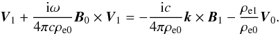16)The perturbation of the charge density can be calculated from the equation ρ_e1 = ∇·E₁/4π. We have with the accuracy in terms of the lowest order in λ/L${\mathit{\rho }}_{\mathrm{e}\mathrm{1}}\mathrm{=}\frac{\mathrm{i}}{\mathrm{4}\mathit{\pi c}}\mathrm{[}{{B}}_{\mathrm{0}}\mathrm{·}\mathrm{(}{k}\mathrm{\times }{{V}}_{\mathrm{1}}\mathrm{)}\mathrm{-}{{V}}_{\mathrm{0}}\mathrm{·}\mathrm{(}{k}\mathrm{\times }{{B}}_{\mathrm{1}}\mathrm{\left)}\mathrm{\right]}\mathit{.}$(17)Substituting Eq. (17) into Eq. (16) and neglecting terms  ~ V²/c², we obtain the second equation, coupling B₁ and V₁, $\mathrm{4}\mathit{\pi c}{\mathit{\rho }}_{\mathrm{e}\mathrm{0}}{{V}}_{\mathrm{1}}\mathrm{+}\mathrm{i}\mathit{\omega }{{B}}_{\mathrm{0}}\mathrm{\times }{{V}}_{\mathrm{1}}\mathrm{+}\mathrm{i}{{V}}_{\mathrm{0}}\mathrm{[}{{B}}_{\mathrm{0}}\mathrm{·}\mathrm{(}{k}\mathrm{\times }{{V}}_{\mathrm{1}}\mathrm{\left)}\mathrm{\right]}\mathrm{=}\mathrm{-}\mathrm{i}{\mathit{c}}^{\mathrm{2}}{k}\mathrm{\times }{{B}}_{\mathrm{1}}\mathit{.}$(18)Two Eqs. (14) and (18) describe the coupled evolution of small perturbations of the velocity and magnetic field.

We study only MHD modes with ω ≪ ck because one can split electromagnetic and hydromagnetic modes in this case. At ω ~ ck, a consideration becomes cumbersome since electromagnetic and hydromagnetic modes are strongly coupled. Apart from this, MHD effects operate basically on a timescale longer than the inverse light frequency, (ck)^-1, because V ≪ c in our model. Therefore, one can expect that MHD instability should be particularly efficient for modes with a relatively low frequency, ω ≪ ck. That is why we consider such modes first.

Estimating B₁ ~ V₁(kB/ω) from Eq. (14), we obtain that the second and third terms on the l.h.s. of Eq. (18) are small compared to the term on the r.h.s. by a factor ω²/c²k². Neglecting these terms on the l.h.s., we have 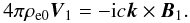$\mathrm{4}\mathit{\pi }{\mathit{\rho }}_{\mathrm{e}\mathrm{0}}{{V}}_{\mathrm{1}}\mathrm{=}\mathrm{-}\mathrm{i}\mathit{c}{k}\mathrm{\times }{{B}}_{\mathrm{1}}\mathit{.}$(19)Modes turn out to be transverse, k·V₁ ≈ 0. Subsituting Eq. (19) into Eq. (14), we obtain 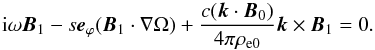$\mathrm{i}\mathit{\omega }{{B}}_{\mathrm{1}}\mathrm{-}\mathit{s}{{e}}_{\mathit{\varphi }}\mathrm{(}{{B}}_{\mathrm{1}}\mathrm{·}\mathrm{\nabla \Omega }\mathrm{)}\mathrm{+}\frac{\mathit{c}\mathrm{(}{k}\mathrm{·}{{B}}_{\mathrm{0}}\mathrm{)}}{\mathrm{4}\mathit{\pi }{\mathit{\rho }}_{\mathrm{e}\mathrm{0}}}{k}\mathrm{\times }{{B}}_{\mathrm{1}}\mathrm{=}\mathrm{0.}$(20)The dispersion equation can be obtained from Eq. (20) in the following way. Calculating a scalar product of Eq. (20) and ∇Ω, we obtain the expression for (B₁·∇Ω) in terms of [B₁·(k × ∇Ω)] . Substituting this expression into Eq. (20), we can express after some algebra B₁ in terms of [B₁·(k × ∇Ω)] . Then, a scalar product of the obtained equation and (k × ∇Ω) yields the dispersion relation in the form ${\mathit{\omega }}^{\mathrm{2}}\mathrm{=}\frac{{\mathit{c}}^{\mathrm{4}}{\mathit{k}}^{\mathrm{2}}\mathrm{(}{k}\mathrm{·}{b}{\mathrm{)}}^{\mathrm{2}}}{{\mathrm{\Omega }}_{\mathrm{m}}^{\mathrm{2}}}\mathrm{-}\mathit{s}\frac{{\mathit{c}}^{\mathrm{2}}\mathrm{(}{k}\mathrm{·}{b}\mathrm{)}}{{\mathrm{\Omega }}_{\mathrm{m}}}\mathrm{[}{{e}}_{\mathit{\varphi }}\mathrm{·}\mathrm{(}{k}\mathrm{\times }\mathrm{\nabla \Omega }\mathrm{\left)}\mathrm{\right]}\mathit{,}$(21)where Ω_m = 4πcρ_e0/B₀ and b = B₀/B₀.

If rotation is rigid and ∇Ω = 0, we obtain the dispersion equation of magnetospheric waves considered by Urpin (2011). Note that in our case k·V₀ = 0 because k has no azimuthal component, whereas V₀ corresponds to rotation and has only the azimuthal component. If |k·b| > k(Ω_m|s∇Ω|/c²k²) the dispersion relation for magnetospheric waves reads 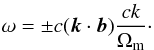$\mathit{\omega }\mathrm{=}\mathrm{\pm }\mathit{c}\mathrm{(}{k}\mathrm{·}{b}\mathrm{)}\frac{\mathit{ck}}{{\mathrm{\Omega }}_{\mathrm{m}}}\mathrm{·}$(22)Since we assume in our consideration that the frequency of magnetohydrodynamic modes should be lower than ck, the magnetospheric modes exists if 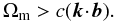${\mathrm{\Omega }}_{\mathrm{m}}\mathit{>}\mathit{c}\mathrm{(}{k}\mathrm{·}{b}\mathrm{)}\mathit{.}$(23)This condition can be satisfied for waves with the wave vector almost (but not exactly) perpendicular to the magnetic field. If the vector k is almost perpendicular to b, it is convenient to denote the angle between k and b in a meridional plane as (π/2 − δ). Then, k·b = kcos(π/2 − δ) ≈ kδψ. Then, Eq. (23) is satisfied if δ < Ω_m/ck.

If rotation is differential and s|∇Ω| > (c²k/Ω_m)(k·b), the properties of magnetospheric waves can be quite different. The first term on the r.h.s. of Eq. (21) is always positive and cannot lead to instability, but the second term can be negative for some k. The instability (ω² < 0) is possible only if the wavevector is almost perpendicular (but not exactly) to the magnetic field and the scalar product (k·b) is small but non-vanishing. Only in this case, the second term on the r.h.s. of Eq. (21) can be greater than the first one. Let us estimate the range of wave vectors that corresponds to unstable perturbations, introducing again the angle between k and b as (π/2 − δ). Substituting this expression into Eq. (21) and estimating [e_ϕ·(k × ∇Ω)]  ~ k|∇Ω|, we obtain that the second term on the r.h.s. of Eq. (21) is greater than the first one if 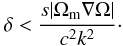$\mathit{\delta }\mathit{<}\frac{\mathit{s}\mathrm{\left|}{\mathrm{\Omega }}_{\mathrm{m}}\mathrm{\nabla \Omega }\mathrm{\right|}}{{\mathit{c}}^{\mathrm{2}}{\mathit{k}}^{\mathrm{2}}}\mathrm{·}$(24)The angle δ turns out to be small, and only perturbations with a wave vector almost perpendicular to B can be unstable.

The instability arises if the second term on the r.h.s. of Eq. (21) is positive. Therefore, the necessary condition of instability reads $\frac{\mathrm{(}{k}\mathrm{·}{b}\mathrm{)}}{{\mathrm{\Omega }}_{\mathrm{m}}}\mathrm{[}{{e}}_{\mathit{\varphi }}\mathrm{·}\mathrm{(}{k}\mathrm{\times }\mathrm{\nabla \Omega }\mathrm{\left)}\mathrm{\right]}\mathit{>}\mathrm{0.}$(25)Since the sign of Ω_m depends on the charge density, the necessary condition is $\mathrm{(}{k}\mathrm{·}{b}\mathrm{)}\mathrm{[}{{e}}_{\mathit{\varphi }}\mathrm{·}\mathrm{(}{k}\mathrm{\times }\mathrm{\nabla \Omega }\mathrm{\left)}\mathrm{\right]}\mathit{>}\mathrm{0} \mathrm{or}\mathit{<}\mathrm{0}$(26)in the region of positive or negative charge density, respectively. It turns out that the necessary conditions (26) can be satisfied by the corresponding choice of the wave vector at any ∇Ω and b. 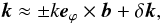Indeed, since k is almost perpendicular to the magnetic field we can represent it as ${k}\mathrm{\approx }\mathrm{\pm }\mathit{k}{{e}}_{\mathit{\varphi }}\mathrm{\times }{b}\mathrm{+}\mathit{\delta }{k}\mathit{,}$(27)where δk is a small component of k parallel (or antiparallel) to b, k ≫ δk (we neglect terms of the order (δk/k)²). Substituting expression (27) into Eq. (26), we obtain for the upper sign with the accuracy in terms linear in δk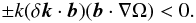$\mathrm{\pm }\mathit{k}\mathrm{(}\mathit{\delta }{k}\mathrm{·}{b}\mathrm{)}\mathrm{(}{b}\mathrm{·}\mathrm{\nabla \Omega }\mathrm{)}\mathit{<}\mathrm{0.}$(28)Obviously, at any sign of (b·∇Ω), one can choose δk in such a way that condition (28) will be satisfied. Condition (26) for the region with a negative charge density can be considered by analogy. Hence, the necessary condition of instability (25) can be satisfied an any differential rotation in the regions of positive and negative charge density.

The characteristic growth rate can be obtained from Eq. (21), using estimate (k·b) ~ kδψ. Then, 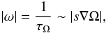$\mathrm{\left|}\mathit{\omega }\mathrm{\right|}\mathrm{=}\frac{\mathrm{1}}{{\mathit{\tau }}_{\mathrm{\Omega }}}\mathrm{~}\mathrm{\left|}\mathit{s}\mathrm{\nabla \Omega }\mathrm{\right|}\mathit{,}$(29)where τ_Ω is the growth time of instability caused by differential rotation. If differential rotation is sufficiently strong and |s∇Ω| ~ Ω, then the growth time of instability is of the order of the rotation period.

4. Discussion

We have considered the instability of a pulsar magnetosphere caused by differential rotation. The consideration was made using the force-free approximation that should be satisfied in the magnetosphere with a high accuracy because the electromagnetic energy density is much greater than the kinetic and thermal energy density. The main result of this study is that the differentially rotating force-free magnetosphere is always unstable. This conclusion is valid for any particular magnetic topology and rotation law. The instability considered in this paper is the representative of a wide class of the magnetorotational instabilities (see, e.g., Velikhov 1959; Balbus & Hawley 1991; Urpin & Rüdiger 2005) modified by the force-free condition and non-vanishing charge density. The typical growth time of the instability can be quite short and can reach the rotation period in the case of a strong differential rotation with |s∇Ω| ~ Ω.

Differential rotation is typical for many models of the magnetosphere. For instance, in the axisymmetric model by Countopoulos et al. (1999) the angular velocity decreases inversely proportional to the cylindrical radius beyond the light cylinder and even stronger in front of it. For this rotation, the growth time of instability should be of the order of the rotation period. Numerical simulations by Komissarov (2006) showed that within the light cylinder, plasma rotates differentially basically near the equator and poles. Therefore, a strong differential rotation should lead to instability arising in these regions. However, the situation can be quite different near the light cylinder where the instability can occur in a much wider region.

The instability considered can be responsible for fluctuations of the magnetospheric emission with the characteristic timescale  ~1/ω. Hydrodynamic motions accompanying the instability can be the reason of turbulent diffusion in the magnetosphere. Note that an influence of the diffusion coefficients should be strongly anisotropic with a much higher enhancement in the direction of the magnetic field since the velocity of motions across the field is much slower than along it.

Despite the force-free condition that substantially reduces the number of modes that can exist in the magnetosphere, there are still many destabilising factors that can lead to instability. Apart from differential rotation, the electric current is likely one more important factor of destabilisation. Note that the topology of the magnetic field can be fairly complicated in the magnetosphere, particularly in a region close to the neutron star. This may happen because the field geometry at the neutron star surface should be very complex (see, e.g., Bonanno et al. 2005, 2006; Urpin & Gil 2004). Therefore, magnetospheric magnetic configurations can be subject to the so-called Tayler instability caused by a distribution of currents. This instability in the pulsar magnetosphere will be considered elsewhere.

Acknowledgments

The author thanks the Russian Academy of Science for financial support under the Programme OFN-15.

References

- Balbus, S., & Hayley, J. 1991, ApJ, 376, 214 [NASA ADS] [CrossRef] [Google Scholar]
- Bonanno, A., & Urpin, V. 2008a, A&A, 477, 35 [NASA ADS] [CrossRef] [EDP Sciences] [Google Scholar]
- Bonanno, A., & Urpin, V. 2008b, A&A, 488, 1 [NASA ADS] [CrossRef] [EDP Sciences] [Google Scholar]
- Bonanno, A., Urpin, V., & Belvedere, G. 2005, A&A, 440, 199 [NASA ADS] [CrossRef] [EDP Sciences] [Google Scholar]
- Bonanno, A., Urpin, V., & Belvedere, G. 2006, A&A, 451, 1049 [NASA ADS] [CrossRef] [EDP Sciences] [Google Scholar]
- Braginskii, S. 1965, Rev. Plasma Phys., 1, 205 [NASA ADS] [Google Scholar]
- Contopoulos, I., Kazanas, D., & Fendt, C. 1999, ApJ, 511, 351 [Google Scholar]
- Davidson, R. 1990, Physics of non-neutral plasmas (Addison-Wesley Publishing Company) [Google Scholar]
- Davidson, R., & Felice, G. 1998. PhPl, 5, 3497 [Google Scholar]
- Fung, P. K., Khechinashvili, D., & Kuijpers, J. 2006, A&A, 445, 779 [NASA ADS] [CrossRef] [EDP Sciences] [Google Scholar]
- Goodwin, S., Mestel, J., Mestel, L., & Wright, G. 2004. MNRAS, 349, 213 [NASA ADS] [CrossRef] [Google Scholar]
- Komissarov, S. 2006, MNRAS, 367, 19 [NASA ADS] [CrossRef] [Google Scholar]
- Levy, R. 1965, PhPl, 8, 1288 [Google Scholar]
- Melrose, D. 1996, Plasma Phys. Control. Fusion, 39, 93 [NASA ADS] [CrossRef] [Google Scholar]
- Mestel, L., & Shibata, S. 1994, MNRAS, 271, 621 [NASA ADS] [Google Scholar]
- Mofiz, U., Amin, M., & Shukla, P. 2012, Astrophys. Space Sci., 337, 177 [NASA ADS] [CrossRef] [Google Scholar]
- Petri, J. 2007, A&A, 469, 843 [NASA ADS] [CrossRef] [EDP Sciences] [Google Scholar]
- Petri, J., Heyvaerts, J., & Bonazzola, S. 2002, A&A, 287, 520 [NASA ADS] [CrossRef] [EDP Sciences] [Google Scholar]
- Petri, J., Heyvaerts, J., & Bonazzola, S. 2003, A&A, 411, 203 [NASA ADS] [CrossRef] [EDP Sciences] [Google Scholar]
- Tayler, R. 1973a, MNRAS, 161, 365 [NASA ADS] [CrossRef] [Google Scholar]
- Tayler, R. 1973b, MNRAS, 163, 77 [NASA ADS] [CrossRef] [Google Scholar]
- Urpin, V. 2011, A&A, 535, L5 [NASA ADS] [CrossRef] [EDP Sciences] [Google Scholar]
- Urpin, V., & Gil, J. 2004, A&A, 415, 305 [NASA ADS] [CrossRef] [EDP Sciences] [Google Scholar]
- Urpin, V., & Rüdiger, G. 2005, A&A, 437, 23 [NASA ADS] [CrossRef] [EDP Sciences] [Google Scholar]
- Velikhov, E. 1959. Sov. Phys. JETP, 9, 995 [Google Scholar]
Current usage metrics show cumulative count of Article Views (full-text article views including HTML views, PDF and ePub downloads, according to the available data) and Abstracts Views on Vision4Press platform.
Data correspond to usage on the plateform after 2015. The current usage metrics is available 48-96 hours after online publication and is updated daily on week days.
Initial download of the metrics may take a while.