| Issue |
A&A
Volume 541, May 2012
|
|
|---|---|---|
| Article Number | A101 | |
| Number of page(s) | 15 | |
| Section | Astronomical instrumentation | |
| DOI | https://doi.org/10.1051/0004-6361/201218774 | |
| Published online | 10 May 2012 | |
Photon orbital angular momentum and torque metrics for single telescopes and interferometers
National Radio Astronomy Observatory, P.V. Domenici Science Operations Center, PO Box O, 1003 Lopezville Road, Socorro, NM 87801-0387, USA ⋆
Received: 4 January 2012
Accepted: 8 March 2012
Abstract
Context. Photon orbital angular momentum (POAM) is normally invoked in a quantum mechanical context. It can, however, also be adapted to the classical regime, which includes observational astronomy.
Aims. I explain why POAM quantities are excellent metrics for describing the end-to-end behavior of astronomical systems. To demonstrate their utility, I calculate POAM probabilities and torques from holography measurements of EVLA antenna surfaces.
Methods. With previously defined concepts and calculi, I present generic expressions for POAM spectra, total POAM, torque spectra, and total torque in the image plane. I extend these functional forms to describe the specific POAM behavior of both single telescopes and interferometers.
Results. POAM probabilities of spatially uncorrelated astronomical sources are symmetric in quantum number. Such objects thus have zero intrinsic total POAM on the celestial sphere, which means that the total POAM in the image plane is identical to the total torque induced by aberrations within propagation media and instrumentation. The total torque can be divided into source- independent and dependent components, and the latter can be written in terms of three illustrative forms. For interferometers, complications arise from discrete sampling of synthesized apertures, but they can be overcome. POAM also manifests itself in the apodization of each telescope in an array. Holography measurements of EVLA antennas observing a point source indicate that ~ 10% of photons in the n = 0 state are torqued to n ≠ 0 states.
Conclusions. POAM quantities represent excellent metrics for characterizing instruments because they are based on real physics and are used to simultaneously describe amplitude and phase aberrations. In contrast, Zernike polynomials are just solutions of a differential equation that happen to ~ correspond to specific types of aberrations (e.g., tip-tilt, focus, etc.) and are typically employed to fit only phases. Possible future studies include forming POAM quantities with real interferometry visibility data, modeling instrumental aberrations and turbulence of the troposphere/ionosphere in terms of POAM, POAM-based imaging algorithms and constraints, POAM-based super resolution imaging, and POAM observations of astrophysically important sources.
Key words: Instrumentation: interferometers / Methods: analytical / Methods: data analysis / Techniques: image processing / Techniques: interferometric / Telescopes
The National Radio Astronomy Observatory is a facility of the National Science Foundation operated under cooperative agreement by Associated Universities, Inc.
© ESO, 2012
1. Introduction
Elias (2008) developed extensive semi-classical formalisms to describe photon orbital angular momentum (POAM) in astronomy. He assumed spatially incoherent sources, so these formalisms are significantly different from those used in laboratory situations. He concentrated more on instrumentation rather than astrophysics, and included first principles, concepts, definitions, calculi, examples, and applications.
As a general rule, aberrations that damage wavefronts and POAM spectra should be minimized in both hardware and software: Primum non torquere1. The amount of damage to wavefronts and POAM spectra should be estimated and removed by off-line image processing algorithms whenever possible. I now extend previous POAM work toward imaging metrics for single telescopes and interferometers, leading to a deeper understanding of how such instruments work.
2. Basic concepts
The apertures of all real astronomical telescopes are finite in size, so they are only capable of producing diffraction-limited images up to a resolution of ~D-1 (D is the aperture diameter expressed in wavelengths). Assuming that the aperture response is uniform or at least azimuthally symmetric (radially apodized), this loss of information manifests itself as blurring. The only rigorous way to reduce blurring is to increase the aperture size.
Conversely, if the aperture response is azimuthally asymmetric (or, azimuthally apodized), the image is subject to non-uniform distortion. These distortions may occur over all angular scales larger than ~D-1. The only rigorous way to reduce distortion is to eliminate the asymmetry in the aperture response.
I distinguish between these two types of image degradation because it is much harder to build a very large telescope compared to figuring a very smooth mirror of nominal size. There is yet another reason for making this distinction, namely that radial apodization does not modulate POAM spectra, while azimuthal apodization does modulate POAM spectra. In other words, aberrations modulate each input POAM state into one or more output POAM states (Elias 2008) and introduce image distortion.
Interferometers measure visibilities at discrete points in the synthesized aperture. In turn, these measurements are transformed into “dirty” images of astronomical sources. This process is mathematically equivalent to punching small pinholes into the opaque aperture of a large single telescope and imaging the resulting interference optomechanically.
The act of aperture sampling is a form of azimuthal apodization that modifies POAM spectra. Other physical effects – including instrumental imperfections, turbulence in the troposphere or ionosphere, etc. – manifest themselves as sample amplitude and phase errors and also modify POAM quantities. Symmetrically reducing the weighting of long baselines, on the other hand, only blurs an image and does not modulate POAM quantities.
I can press the analogies even further. Image-processing algorithms, such as CLEAN and MEM, remove artifacts to yield a model of the true source up to a certain resolution. These artifacts are produced by asymmetric apodization, which means that image-processing algorithms actually estimate and eliminate changes in POAM spectra.
3. Definitions
According to Elias (2008), the total POAM of a wavefront arising from the celestial sphere, in units of ħ, is  (1a)where
  (1b)is the probability that a single photon (or the fraction of many photons) is in POAM state m, Bm,m is the (m,m)th POAM autocorrelation, and B is the total intensity. The ensemble of probabilities represents the intrinsic source POAM spectrum. The total intensity, which is integrated over the celestial sphere, is identical to the sum over all POAM autocorrelations. The same formulae can be used to describe the total POAM of a wavefront incident upon the image plane by replacing lZ →
  , LZ →
  , pm,m →
  , Bm,m →
  , and B →
  .
.
I define the total torque as the difference of the total POAM between the image plane and celestial sphere, or  (2)where the ensemble of τm,m comprise the torque spectrum. Torque is normally defined as change in angular momentum per unit time. Since “per unit time” is ambiguous in this context I ignore it, so torque has the same units as POAM.
The electric fields of a “natural light” astronomical source projected onto the celestial sphere are spatially uncorrelated. I call this scenario the “standard astronomical assumption” (SAA), which led to the creation of the POAM calculi (Elias 2008; Tables 1 − 4). Because of SAA, B − m, − m = Bm,m and p − m, − m = pm,m for all m, implying that lZ = 0. I derive this result in Appendix A. Equation (2) then becomes  (3)Torque applied by propagation media and instrumentation modifies the source POAM spectral components as they travel to the image plane, but the total POAM in the image plane does not depend on the total POAM from the celestial sphere because of the symmetry in m. Although this equation is independent of lZ, the ± 1 transitional probabilities of the source do affect (cf. Sect. 4) except for point sources at the center of the field of view (FOV).
Maser photons traveling through turbulent gas and photons scattering off Kerr black holes (Harwit 2003; Tamburini et al. 2011) may not satisfy the SAA condition. Therefore, these sources can exhibit lZ ≠ 0 and are beyond the scope of this paper.
4. Single telescopes
I derive POAM quantities for single telescopes first because it is relatively simple to do and the results can be extended to other types of instruments (e.g., interferometers; cf. Sect. 5). Elias (2008) created generic calculi that can describe the POAM response of any instrument, so I will use them here.
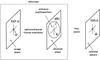 |
Fig. 1 Schematic diagram of a single telescope looking at a source on the celestial sphere. The coordinates are indicated and described in the text of Sect. 4. The electric fields (celestial sphere and image plane) and aperture function are also presented. |
4.1. Initial mathematics
Consider Fig. 1, the schematic diagram of a single telescope looking at an object on the celestial sphere. The intensity response, in system form, for an SAA source is given by 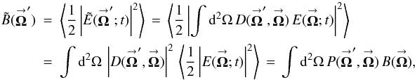 (4a)where
  = (ρcosφ,ρsinφ) is the coordinate on the celestial sphere,
  = (ρ′cosφ′,ρ′sinφ′) is the coordinate in the image plane,
  and
and  are the intensity distributions (
 and
and  are the corresponding electric fields),
  =
=  is the point-spread function (PSF),
 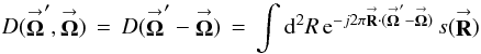 (4b)is the diffraction function (DF),
  = (Rcosψ,Rsinψ) is the coordinate in the aperture (in units of wavelength), and
  is the functional description of the aperture apodization (cf. Sect. 2). Any optical system, including propagation media and instrumentation, that can be expressed in this mathematical form can be expanded into any of the POAM calculi.
From Elias (2008; row 3 of Table 3), the (m,m)th single-telescope SAA POAM autocorrelation density is 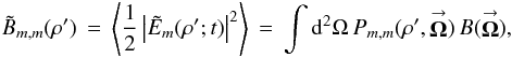 (5a)where
  (5b)is the mth image-plane POAM state,
 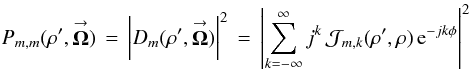 (5c)is the (m,m)th PSF sensitivity,
  (5d)is the mth DF sensitivity,
 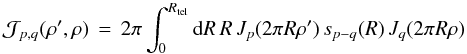 (5e)is the (p,q)th integral function, Rtel is the telescope radius, Jg(x) is the gth order Bessel function of the first kind, and
 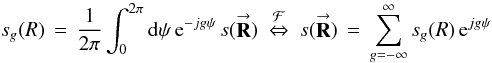 (5f)is the gth azimuthal Fourier component of the aperture function . Integrating Eq. (5a) over radius in the image plane leads to the (m,m)th POAM autocorrelation
  (6a)where ρFOV is the FOV of the image plane, and
  (6b)is the (m,m)th PSF sensitivity kernel. I assume that ρFOV is large enough to capture most of the radiation scattered through the telescope aperture into the image plane. The complete derivation of Eqs. (5), (6) may be found in Appendix B.
All POAM quantities defined in Sect. 3 can be formed from Eqs. (6a), (b). For example, the total POAM in the image plane is ![Mathematical equation: \begin{eqnarray} \label{Eq:TildeLz} \tilde{l}_{Z} \, = \, \frac{1}{\tilde{B}} \sum_{m=-\infty}^{\infty} m \, \tilde{B}_{m,m} \, = \, \frac{1}{\tilde{B}} \int {\rm d}^{2}\Omega \, \left[ \sum_{m=-\infty}^{\infty} m \, P_{m,m}(\vecbf{\Omega}) \right] \, B(\vecbf{\Omega}) \, = \, \frac{1}{\tilde{B}} \int {\rm d}^{2}\Omega \, \tilde{\mathcal{L}}_{z}(\vecbf{\Omega}) \, B(\vecbf{\Omega}) , \end{eqnarray}](/articles/aa/full_html/2012/05/aa18774-12/aa18774-12-eq61.png) (7)where
(7)where  is the total POAM kernel. Total POAM on the celestial sphere for all SAA sources is identically zero, or lZ = 0 (cf. Appendix A). This statement means that the total POAM measured in the image plane is identical to total torque applied to the wavefronts. Therefore, I interchangably employ the quantities ↔ τ and ↔
  , where is the total torque kernel. For a more physical understanding of Eq. (7), Eqs. (6a), (b) are combined with various mathematical identities to create three “illustrative forms” of which emphasize different aspects of POAM for single telescopes (cf. Sect. 4.2).
4.2. Illustrative forms of l˜Z
The first illustrative form of is ![Mathematical equation: \begin{eqnarray} \label{Eq:TelTorque1} \tilde{l}_{Z} = \sum_{m=-\infty}^{\infty} m p^{a}_{m,m} \pm \mathrm{Im} \, 2\pi \int_{0}^{\infty} {\rm d}\rho \, \rho \, 2\pi \int_{0}^{R_{\rm tel}} {\rm d}R \, R \, \left( 2\pi R \rho \right) \left[ \sum_{n=-\infty}^{\infty} p_{n,n \pm 1}(\rho) \right] \left[ \sum_{m=-\infty}^{\infty} p^{a}_{m,m \mp 1}(R) \right] , \end{eqnarray}](/articles/aa/full_html/2012/05/aa18774-12/aa18774-12-eq67.png) (8)where
(8)where  is the mth POAM state probability in the aperture, pn,n ± 1(ρ) is the transitional probability density between POAM states n and n ± 1 on the celestial sphere, and
  is the transitional probability density between POAM states m and m ∓ 1 in the aperture. The transitional probabilities correspond to ± 1 selection rules. I derive these equations and the variables contained therein in Appendix C.
The second illustrative form of is ![Mathematical equation: % subequation 1252 0 \begin{equation} \label{Eq:TelTorque2} \tilde{l}_{Z} \, = \, \sum_{m=-\infty}^{\infty} m \, p^{a}_{m,m} \, \pm \, \mathrm{Im} \, 2\pi \int_{0}^{\infty} {\rm d}\rho \, \rho ~ 2\pi \int_{0}^{R_{\rm tel}} \, {\rm d}R \, R \, \left( 2\pi R \rho \right) \, \left[ \frac{\mathcal{B}_{\mp 1}(\rho)}{B} \right] \left[ \frac{\mathcal{S}_{\pm 1}(R)}{S} \right] \end{equation}](/articles/aa/full_html/2012/05/aa18774-12/aa18774-12-eq73.png) (9a)where the ℬ ∓ 1(ρ) are the first order rancors of the source, the
(9a)where the ℬ ∓ 1(ρ) are the first order rancors of the source, the  are the first order rancor sensitivities, and S is the integrated squared magnitude of the aperture function. This expression proves that rancors and rancor sensitivities (Elias 2008),
 ![Mathematical equation: % subequation 1252 1 \begin{equation} \label{Eq:R22} \mathcal{B}_{p}(\rho) = \frac{1}{2\pi} \int_{0}^{2\pi} {\rm d}\phi \, {\rm e}^{-jp\phi} \, B(\vecbf{\Omega}) = \sum_{m=-\infty}^{\infty} B_{m,m-p}(\rho) ~~\, \stackrel{\mathcal{F}}{\Leftrightarrow} ~~ B(\vecbf{\Omega}) \, = \, \sum_{p=-\infty}^{\infty} \mathcal{B}_{p}(\rho) \, {\rm e}^{jp\phi} ~~~~ \left[ B_{i,k}(\rho) \, = \, \left< \frac{1}{2} E_{i}(\rho;t) E^{*}_{k}(\rho;t) \right> \right], \end{equation}](/articles/aa/full_html/2012/05/aa18774-12/aa18774-12-eq77.png) (9b)and
(9b)and ![Mathematical equation: % subequation 1252 2 \begin{equation} \label{Eq:R2} \mathcal{S}_{p}(R) = \frac{1}{2\pi} \int_{0}^{2\pi} {\rm d}\psi \, {\rm e}^{-jp\psi} \, S(\vecbf{R}) = \sum_{m=-\infty}^{\infty} S_{m,m-p}(R) ~~\, \stackrel{\mathcal{F}}{\Leftrightarrow} ~~ S(\vecbf{R}) \, = \, \sum_{p=-\infty}^{\infty} \mathcal{S}_{p}(R) \, {\rm e}^{jp\psi} ~~~~ \left[ S_{i,k}(R) \, = \, s_{i}(R) s^{*}_{k}(R) , ~ S(\vecbf{R}) \, = \, \left|s(\vecbf{R})\right|^2 \right] , ~ \end{equation}](/articles/aa/full_html/2012/05/aa18774-12/aa18774-12-eq78.png) (9c)calculated directly from intensities and squared aperture functions (instead of electric fields and aperture functions) and related to the transitional probabilities of Eq. (8), are relevant for POAM analysis. I derive these equations and the variables contained therein in Appendix C.
(9c)calculated directly from intensities and squared aperture functions (instead of electric fields and aperture functions) and related to the transitional probabilities of Eq. (8), are relevant for POAM analysis. I derive these equations and the variables contained therein in Appendix C.
The third illustrative form of is ![Mathematical equation: \begin{equation} \label{Eq:TelTorque3} \tilde{l}_{Z} \, = \, \sum_{m=-\infty}^{\infty} m \, p^{a}_{m,m} \, + \, 2\pi \int {\rm d}^{2}\Omega \int {\rm d}^{2}R \, \left[ \vecbf{\Omega} \, \times \, \vecbf{R} \right] \, p(\vecbf{\Omega}) \, p^{a}(\vecbf{R}) \, = \, \sum_{m=-\infty}^{\infty} m \, p^{a}_{m,m} \, + \, 2\pi \left[ \int {\rm d}^{2}\Omega \, \vecbf{\Omega} \, p(\vecbf{\Omega}) \right] \, \times \, \left[ \int {\rm d}^{2}R \, \vecbf{R} \, p^{a}(\vecbf{R}) \right] , \end{equation}](/articles/aa/full_html/2012/05/aa18774-12/aa18774-12-eq79.png) (10)where
(10)where  is the probability that a photon can pass through the aperture within d2R of , and
  is the probability that a photon arose from the celestial sphere within d2Ω of . The source-dependent term is expressed as × operating on the probabilities or the cross product of the dipole moments of the probabilities. I derive these equations and the variables contained therein in Appendix C.
For an on-axis point source (ρ = 0), the POAM and torque spectra in the image plane are identical to the source-independent POAM spectra within the aperture, or 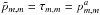 . Even if the object under observation is not an on-axis point source, the ensemble of
  and the POAM quantities formed from them represent reasonable source-independent metrics.
The source-dependent terms, on the other hand, are dipole moments with ± 1 selection rules, which means that they are identically zero on-axis and their effects are relatively small off axis. Elias (2008) called these terms “pointing” POAM or “structure” POAM. The source structure cannot be easily disentangled from the effects of propagation media and instrumentation. They are also zero when there is only a single non-zero sk(R).
5. Interferometers
Elias (2008) derived POAM correlations and rancors for a single-baseline optical interferometer. They depend on baseline length, delay, telescope aberrations, etc. Since he was considering only a single observation with a single pair of telescopes and integrating over the image plane, employing the baseline vector instead of the two telescope vectors is acceptable. For this simple situation, the total POAM and torque can be set to zero because the synthetic aperture origin can be always placed along the line containing the single correlation measurement of two telescopes.
In this section, I derive image-plane POAM quantities for an interferometer. There are slight differences between radio and optical interferometry. In the radio case, the electric fields between pairs of telescopes are multiplied and averaged. In the optical case, electric fields are summed, squared, and averaged. Mathematically, the same zero-spacing fluxes and visibilities can be obtained in both the radio and optical. I assume that the fringes are tracked well enough to avoid any delay dependence.
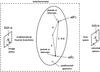 |
Fig. 2 Schematic diagram of an interferometer looking at a source on the celestial sphere. The coordinates are indicated and described in the text of Sects. 4 and 5. The electric fields (celestial sphere and image plane) and aperture function are also presented. The aperture function refers to the synthesized aperture, not to the individual telescope (or pinhole) apertures that sample it. |
Consider a single telescope behind an opaque aperture that contains a finite number of imperfect pinholes with amplitude and phase errors. The resulting “dirty” image is the convolution of the perfect diffraction-limited image and the Fourier transform of the imperfect pinhole pattern, which is equivalent to the “optomechanical” Fourier transform of the unnormalized visibilities from all pinhole pairs. An interferometer works in a similar manner. Multiple observations with an array of small telescopes, representing the imperfect pinholes, form the “synthesized” aperture of a single large telescope (cf. Fig. 2). Unnormalized visibilities of all telescope pairs are then mathematically Fourier transformed to create the dirty image. The sky-dependent response of the individual telescopes defines the image FOV and their imperfections also affect the images (cf. Sects. 5.2 and 6).
5.1. Initial mathematics
The single-telescope POAM mathematics of Sect. 4.1 can be used directly with interferometers, taking into account the discrete sampling of the aperture. For the sake of illustration, however, I rewrite them in terms of sampled unnormalized visibilities, which are the standard interferometer observables. The interferometer intensity response is ![Mathematical equation: % subequation 1530 0 \begin{eqnarray} \label{Eq:IntResponse} \tilde{B}(\vecbf{\Omega}^{\prime}) &= &\left< \frac{1}{2} \left| \tilde{E}(\vecbf{\Omega}^{\prime};t) \right|^{2} \right> \, = \, \left< \frac{1}{2} \left| \int {\rm d}^{2}R^{\prime} \, {\rm e}^{-j 2\pi \vecbf{R}^{\prime} \cdot \vecbf{\Omega}^{\prime}} \, s(\vecbf{R}^{\prime}) \, \mathcal{E}(\vecbf{R}^{\prime};t) \right|^{2} \right> \nonumber \\ &= &\int {\rm d}^{2}R^{\prime} \, \int {\rm d}^{2}R \, {\rm e}^{-j 2\pi (\vecbf{R}^{\prime}-\vecbf{R}) \cdot \vecbf{\Omega}^{\prime}} \, \left[ s(\vecbf{R}^{\prime}) \, s^{*}(\vecbf{R}) \, \mathcal{F}(\vecbf{R}^{\prime},\vecbf{R}) \right] \, = \, \int {\rm d}^{2}R^{\prime} \, \int {\rm d}^{2}R \, {\rm e}^{-j 2\pi (\vecbf{R}^{\prime}-\vecbf{R}) \cdot \vecbf{\Omega}^{\prime}} \, \tilde{\mathcal{F}}(\vecbf{R}^{\prime},\vecbf{R}) , ~~~~~~~~ \end{eqnarray}](/articles/aa/full_html/2012/05/aa18774-12/aa18774-12-eq90.png) (11a)where
(11a)where  is the electric field in the synthesized aperture,
  is the telescope-based gain function of the synthesized aperture (analogous to the aperture function of a single telescope, cf. Sect. 4),
  is the uncalibrated unnormalized visibility, and
  (11b)is the true unnormalized visibility under SAA. Note that the image-plane intensity of Eq. (11a) is expressed in terms of two aperture-plane integrals, as opposed to the standard single integral over baseline
  =
=  − (the separation of two telescopes), because POAM quantities depend on telescope position vectors not baseline vectors. In Appendix D, I prove that this equation can be converted to the baseline form used for non-POAM analysis. I assume that a single moving baseline produces all of the unnormalized visibilities. All formulae, however, can easily be generalized to multiple moving baselines.
Expanding the exponential functions in Eq. (11a) in terms of Bessel functions, the (m,m)th POAM autocorrelation density becomes  (12a)Integrating over the image plane, I obtain the (m,m)th POAM autocorrelation
  (12b)where
  and Rint is the radius of the synthesized aperture, both in units of wavelength. These equations are derived in Appendix D. As in the single-telescope case (cf. Sect. 4.1), Eq. (12b) can be used to create all of the POAM quantities defined in Sect. 3 as well as the illustrative forms of Sect. 4.2 (cf. Appendix D). There are, however, two complications.
The only uncalibrated unnormalized visibilities that contribute to the mth POAM state autocorrelations are those which come from pairs of telescopes in the same aperture ring R, i.e., pairs of telescopes that are the same distance from the aperture reference point ( , cf. Fig. 2). This result is not surprising given that POAM quantities are defined in rings. As a matter of fact, it is possible to rewrite Eq. (12b) as azimuthal Fourier series components of the azimuthal convolution of uncalibrated aperture electric fields integrated over radius. Unfortunately, real interferometers do not have telescopes arranged in this manner, which means that the true unnormalized visibilities and telescope-based gains must somehow be interpolated onto a polar grid.
Single telescopes obtain data using an entire aperture. Source-independent POAM quantities calculated from an on-axis point source calibrator observation can be used to judge the quality of separate science target observations if the atmospheric statistics are ≈ consistent and the source structure does not extend too far from the FOV center. This strategy does not work for interferometers. They obtain data through a sampled synthetic aperture, so the sample coverage for an on-axis point source calibrator and a science target will be different.
Determining the optimum strategy to overcome these complications requires a significant amount of effort. Such work is beyond the scope of this paper, but here I present two possible candidates that act as starting points for future research.
When the ungridded discrete Fourier transform (DFT) of science target uncalibrated unnormalized visibilities is calculated (no additional processing; e.g., CLEAN), the resulting image is corrupted by incomplete sampling of the synthetic aperture and gain errors. If the inverse DFT (IDFT) of the corrupted image is calculated on a polar grid, it effectively interpolates the uncalibrated unnormalized visibilities so that they can be used directly in Eq. (12a) to form the POAM quantities of Sects. 3 and 4.
Many interferometry imaging-processing techniques iteratively solve for sampled true unnormalized visibilities and telescope-based gains while improving the image model (Rau et al. 2009; Rau 2010). If the synthetic aperture is sampled densely enough, the true unnormalized visibilities and telescope-based gains can be interpolated onto a uniform polar grid so that the desired POAM quantities of Sects. 3 and 4 can be determined. In Appendix E, I show that the interpolation kernel must be azimuthally symmetric, or  , in order not to further modulate the POAM spectrum.
These two strategies yield different results. The DFT/IDFT interpolation method includes the effects of both incomplete sampling and gain errors. The azimuthally symmetric interpolation kernel method, on the other hand, includes only the effects of gain errors if the processing successfully removes artifacts due to imperfect synthesized aperture sampling. The DFT/IDFT interpolation method includes pointing/structure POAM which cannot be easily disentangled from source-independent terms (if the object under observation is an on-axis point source, there is no pointing/structure POAM). Conversely, the azimuthally symmetric interpolation kernel method estimates the aperture functions, which means that pointing/structure POAM can be disentangled from source-independent terms.
5.2. Telescope apodization
The true unnormalized visibility (Eq. (11b)) for a single baseline, modified by the apodization of the individual telescopes, is ![Mathematical equation: \begin{eqnarray} \label{Eq:SkyVisApod} \mathcal{F}(\vecbf{R}^{\prime},\vecbf{R}) \, = \, \int {\rm d}^{2}\Omega \, {\rm e}^{j 2\pi (\vecbf{R}^{\prime}-\vecbf{R}) \cdot \vecbf{\Omega}} \, \left[ \mathcal{A}^{\prime}(\vecbf{\Omega}) \, \mathcal{A}^{*}(\vecbf{\Omega}) \right] \, B(\vecbf{\Omega}) \, = \, \int {\rm d}^{2}\Omega \, {\rm e}^{j 2\pi (\vecbf{R}^{\prime}-\vecbf{R}) \cdot \vecbf{\Omega}} \, \mathcal{P}(\vecbf{\Omega}) \, B(\vecbf{\Omega}) , ~~ \end{eqnarray}](/articles/aa/full_html/2012/05/aa18774-12/aa18774-12-eq105.png) (13)where
(13)where  and
and  are the complex electric-field sky-dependent gains of the two telescopes at points and in the observation plane, and
  is their combined power sky-dependent gain. This equation can easily be generalized for multiple moving baselines. If the electric-field gains are identical, the power gain is real. If the converse is true, the power gain is complex. A complex power gain represents a non-Hermitian calibration error,
  ≠
≠  , which leads to a complex output image (cf. Eq. (14)).
Substituting Eq. (13) into Eqs. (11a), (11b), I obtain a modified version of Eq. (4a)  (14)When expanded into POAM components, Eq. (14) becomes
  (15a)where the POAM correlations
 ![Mathematical equation: % subequation 1884 1 \begin{equation} \label{Eq:TelResponseAPOAM} \tilde{B}_{p,q}(\rho^{\prime}) \, = \, \sum_{m=-\infty}^{\infty} \sum_{n=-\infty}^{\infty} 2\pi \int_{0}^{\infty} {\rm d}\rho \, \rho \left[ \sum_{k=-\infty}^{\infty} \sum_{l=-\infty}^{\infty} P_{p,q}^{-k,-l}(\rho^{\prime},\rho) \, \mathcal{P}_{k-l-m+n}(\rho) \right] \, B_{m,n}(\rho) \end{equation}](/articles/aa/full_html/2012/05/aa18774-12/aa18774-12-eq113.png) (15b)have an extra function
(15b)have an extra function  (15c)The interferometric PSF input/output (separate) gain is
  (16a)where
  (16b)is the interferometric DF input/output gain. These gains are defined in Tables 2 and 4 of Elias (2008). I derive Eqs. (15b, c) in Appendix F.
From Eq. (15b), I see that sky-dependent gains do indeed modulate POAM. To understand these effects more clearly, I choose a simple case where the interferometric synthetic aperture is fully sampled with no amplitude or phase errors, which means that  (17a)(Elias 2008). Equation (15b) then becomes
 ![Mathematical equation: % subequation 1962 1 \begin{equation} \label{Eq:TelResponseAPOAMpqpq} \tilde{B}_{p,q}(\rho^{\prime}) \, = \, \sum_{m=-\infty}^{\infty} \sum_{n=-\infty}^{\infty} 2\pi \int_{0}^{\infty} {\rm d}\rho \, \rho \left[ P_{p,q}^{-p,-q}(\rho^{\prime},\rho) \, \mathcal{P}_{p-q-m+n}(\rho) \right] \, B_{m,n}(\rho) . \end{equation}](/articles/aa/full_html/2012/05/aa18774-12/aa18774-12-eq118.png) (17b)Now only the sky-dependent gains distribute the input POAM correlation densities to multiple output POAM correlation densities. The index of the extra function consists of the difference of image plane and celestial sphere index differences. To further verify that these mathematics are correct, I let the sky-dependent gain exhibit only radial apodization, or
(17b)Now only the sky-dependent gains distribute the input POAM correlation densities to multiple output POAM correlation densities. The index of the extra function consists of the difference of image plane and celestial sphere index differences. To further verify that these mathematics are correct, I let the sky-dependent gain exhibit only radial apodization, or  . The new extra function
  (18a)produces a one-to-one correspondence between input and output POAM correlation densities
 ![Mathematical equation: % subequation 1998 1 \begin{equation} \label{Eq:TelResponseAPOAMmn} \tilde{B}_{m,n}(\rho^{\prime}) \, = \, 2\pi \int_{0}^{\infty} {\rm d}\rho \, \rho \, \left[ \sum_{p=-\infty}^{\infty} P_{p,p-m+n}^{-p,-p+m-n}(\rho^{\prime},\rho) \right] \, \mathcal{P}_{0}(\rho) \, B_{m,n}(\rho) . \end{equation}](/articles/aa/full_html/2012/05/aa18774-12/aa18774-12-eq121.png) (18b)as expected.
(18b)as expected.
The sky-dependent gain for each antenna can be determined via holography, i.e., raster scans around a bright point source normalized (amplitude and phase) to a reference antenna (cf. Sect. 6).
The Fourier transforms of the sky-dependent gains and their inverses are  (19)where
  and
and  are the complex holography functions representing aperture imperfections projected back to planes in front of the telescopes. The aperture coordinates are
  = (r′cosχ′,r′sinχ′) and
  = (rcosχ,rsinχ). These functions are conceptually identical to the single-telescope aperture function (cf. Sect. 4.1) and interferometer synthesized aperture function (cf. Sect. 5.1). The POAM components of the inverse transforms are
  (20a)where
  (20b)and
  (20c)Note that when the apertures are azimuthally symmetric, or → a′(r′) =
  and → a(r) = a0(r), only the
  and
and  terms are non-zero. Further, if both antennas of a baseline are azimuthally symmetric, it follows that their power pattern is also azimuthally symmetric →
  =
= 
 and does not redistribute POAM states.
6. EVLA holography and POAM
Recent K-band ( ≈ 24 GHz) holography observations of EVLA antennas were processed during commissioning2 (Brentjens 2011). The target is a bright point source. Three of the antennas tracked the target and were used as amplitude and phase references. The rest of the antennas – i.e., those under test – executed raster scans. The resulting data were flagged, calibrated, and averaged before calculating the Fourier transforms on Cartesian and polar output coordinates. Calibration included removing the effects of pointing, focus, and subreflector rotation offset, so the holography should ~represent the imperfections of the antenna surfaces.
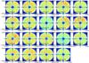 |
Fig. 3 Holographic amplitude measurements of the EVLA antennas. The blue and red colors represent the low and high reflectivity regions. The coordinate units are wavelengths. |
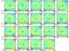 |
Fig. 4 Holographic phase measurements of the EVLA antennas. The yellow colors represent raised regions with respect to the fiducial dish surfaces. The rms panel deviations are ≈ 200 μm. The coordinate units are wavelengths. |
The amplitude and phase responses (Cartesian coordinates) are shown in Figs. 3 and 4. When calculating the Fourier transforms, I oversampled the output by a factor of six for smoother interpolation. The circular shape of the dishes is clearly visible. The amplitude responses exhibit an opaque region near the center and four orthogonal “spokes” produced by the subreflector and its supports. There are also clear indications of both large and small spatial scale reflectivity features. The phase responses show random phases in the opaque regions, as expected. The locations of the small scale phase features (mottled patterns) are consistent with individual misaligned panels on the reflector surface. They tend to appear in groups.
 |
Fig. 5 Holographic probability spectra of the EVLA antennas. The ordinates are log (base 10) probability/100% and the abscissae are POAM states. The total torque is written on each subplot. |
In Fig. 5, I display the sky-independent image-plane POAM probability spectra (corresponding to the aperture POAM probability spectra in Eqs. (8), (9a), and (10)) as well as the total torques. There are no sky-dependent quantities (i.e., no pointing/structure POAM) because the object under observation is an on-axis point source. To determine the sky-independent image-plane probabilities for each telescope, I calculate the azimuthal Fourier series components of its aperture function versus radius  , form the squared magnitude of each Fourier component versus radius
  , sum each squared magnitude over radius to obtain |ak|2 (times 2πr Δr, where Δr is the radial size of the aperture element), and normalize the |ak|2 to the sum of the |ak|2 over k. The range of POAM components is limited to ± 15, which is ≈ the Nyquist limit at the largest radius (I do not calculate higher POAM components even though they are available because of oversampling).
When a perfect telescope observes an on-axis point source only the n = 0 component of the image-plane POAM spectrum is non-zero. Conversely, when an imperfect telescope observes an on-axis point source the n = 0 component is reduced and the other components become non-zero. Most of the n ≠ 0 probabilities are 1% or less. A few of the n = ± 1 probabilities are almost an order of magnitude larger, which could be caused by feed position errors or uncalibrated pointing errors. Summing over the n ≠ 0 probabilities, we find that ~10% of all photons are “torqued” away from the n = 0 state. Also, note that most telescopes exhibit a non-zero total torque but some (e.g., telescopes 24 and 28) exhibit ≈ zero total torque (i.e., ≈symmetric POAM spectra).
7. Conclusion
With previously defined concepts and calculi (Elias 2008), I presented generic expressions for POAM spectra, total POAM, torque spectra, and total torque in the image plane. I extended these functional forms to describe the specific POAM behavior of both single telescopes and interferometers. These POAM quantities make excellent metrics, complimenting Zernike polynomials, for describing the response of astronomical instruments. Real holography measurements of EVLA antennas demonstrated their utility.
Now that POAM metrics have been derived, it is incumbent on the author to make them available to the astronomical community in an imaging package. In the future, I plan to extend them to handle spin-polarized and non-flat spectrum sources. Possible future studies include forming POAM quantities using real interferometry visibility data, modeling instrumental aberrations and turbulence of the troposphere/ionosphere in terms of POAM, POAM-based imaging algorithms and constraints, POAM-based super resolution imaging (Tamburini et al. 2006) without interpolation or extrapolation, and POAM observations of astrophysically important sources such as masers and black holes (Harwit 2003; Tamburini et al. 2011).
The National Radio Astronomy Observatory is a facility of the National Science Foundation operated under cooperative agreement by Associated Universities, Inc.
This Latin phrase – loosely translated as “Above all, apply no torque” – is a shameless adaptation of the most widely quoted words from the Hippocratic Oath “Primum non nocere,” which means “Above all, do no harm”.
Observing program THOL0001, source 3C 273, 2011 October 14.
Acknowledgments
NME2 would like to thank Dr. Sanjay Bhatnagar for fruitful discussions and advice, and Drs. Michiel Brentjens, Richard A. Perley, and Bryan J. Butler for providing calibrated EVLA holography data. NME2 would also like to thank the anonymous referee for his practical and philosophical comments.
References
- Elias II, N. M. 2008, A&A, 492, 883 [NASA ADS] [CrossRef] [EDP Sciences] [Google Scholar]
- Harwit, M. 2003, ApJ, 597, 1266 [NASA ADS] [CrossRef] [Google Scholar]
- Brentjens, M. 2011, unpublished EVLA holography data [Google Scholar]
- Rau, U. 2010, Ph.D. Thesis, New Mexico Institute of Mining and Technology [Google Scholar]
- Rau, U., Bhatnagar, S., Voronkov, M. A., & Cornwell, T. J. 2009, IEEE, 97, 1472 [Google Scholar]
- Tamburini, F., Anzolin, G., Umbriaco, G., Bianchini, A., & Barbieri, C. 2006, Phys. Rev. Lett., 97, 163903 [NASA ADS] [CrossRef] [Google Scholar]
- Tamburini, F., Thidé, B., Molina-Terriza, G., & Anzolin, G. 2011, Nat. Phys., 7, 195 [Google Scholar]
Appendix A: POAM from the celestial sphere
Elias (2008) tacitly assumed that the total POAM on the celestial sphere was zero for SAA sources and non-zero for non-SAA sources. In this appendix, I formally prove those statements for a single telescope, but the derivations apply to all optical systems, including interferometers.
I consider the SAA case first. If the instrument does not modulate the POAM spectrum, the aperture function in Eq. (5f) becomes = s0(R). The integral function in Eq. (5e) then simplifies to  =
=  δq,p. When this result is substituted into Eq. (5c), the (m,m)th POAM sensitivity is no longer a function of φ, or
  → Pm,m(ρ′,ρ) =
  . Upon inspection of Eq. (5e), I find that
  =
=  , which means that P − m, − m(ρ′,ρ) = Pm,m(ρ′,ρ). Since Pm,m(ρ′,ρ) is even in m, the total image-plane POAM of Eq. (7) is identically zero. Because I initially assumed that the instrument does not modulate POAM, it follows that the total POAM on the celestial sphere must be zero as well. Further, the total POAM on the celestial sphere for SAA sources must always be zero because the behavior of the source must be completely independent of the behavior of the instrument. Q.E.D.
I now consider the non-SAA case using a completely spatially correlated source. The spatial and temporal parts of the electric field on the celestial sphere factor into separate functions, =  f(t), where f(t) is a random complex function. The electric field in the image plane (Eq. (4a)) becomes
 ![Mathematical equation: \appendix \setcounter{section}{1} % subequation 2670 0 \begin{equation} \label{Eq:TelResponse2} \tilde{E}(\vecbf{\Omega}^{\prime};t) \, = \, \int {\rm d}^{2}\Omega \, D(\vecbf{\Omega}^{\prime},\vecbf{\Omega}) \, E(\vecbf{\Omega};t) \, = \, \left[ \int {\rm d}^{2}\Omega \, D(\vecbf{\Omega}^{\prime},\vecbf{\Omega}) \, E(\vecbf{\Omega}) \right] \, f(t) \, = \, \tilde{E}(\vecbf{\Omega}^{\prime}) \, f(t) . \end{equation}](/articles/aa/full_html/2012/05/aa18774-12/aa18774-12-eq163.png) (A.1a)Expanding the DF into sensitivities (Eq. (5d)) yields
(A.1a)Expanding the DF into sensitivities (Eq. (5d)) yields ![Mathematical equation: \appendix \setcounter{section}{1} % subequation 2670 1 \begin{equation} \label{Eq:TelResponse3} \tilde{E}(\vecbf{\Omega}^{\prime};t) \, = \, \sum_{m=-\infty}^{\infty} \tilde{E}_{m}(\rho^{\prime};t) \, {\rm e}^{jm \phi^{\prime}} \, = \, \sum_{m=-\infty}^{\infty} \left[ \tilde{E}_{m}(\rho^{\prime}) \, f(t) \right] \, {\rm e}^{jm \phi^{\prime}} \, = \, \sum_{m=-\infty}^{\infty} \left[ \int {\rm d}^{2}\Omega \, D_{m}(\rho^{\prime},\vecbf{\Omega}) \, E(\vecbf{\Omega}) \, f(t) \right] \, {\rm e}^{jm \phi^{\prime}} . ~~~~~~ \end{equation}](/articles/aa/full_html/2012/05/aa18774-12/aa18774-12-eq164.png) (A.1b)Apart from the separation of the spatial and temporal components of the electric field and the POAM states, these functional forms are identical to the SAA ones.
(A.1b)Apart from the separation of the spatial and temporal components of the electric field and the POAM states, these functional forms are identical to the SAA ones.
With these POAM states, I form the image-plane POAM autocorrelation densities (Eq. (5a)) and express the PSF sensitivities in terms of the integral functions (Eq. (5c))  (A.2a)where F =
  is the rms of the random complex function. Again I assume that the instrument does not modulate POAM, or
  = δk,m, thereby collapsing the sum in this equation. Combining this fact with integration over radius ρ′ in the image plane, I obtain the total (m,m)th POAM autocorrelation in the image plane
 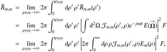 (A.2b)where
 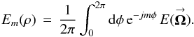 (A.2c)This equation shows that
  ≠ because E − m(ρ) ≠ Em(ρ) in general, which means that the total image-plane POAM can be non-zero (Eq. (3)). The total image-plane POAM is the same as the total source POAM because the instrument does not modulate POAM, so if the former is non-zero the latter must be non-zero as well. Q.E.D.
In the previous two proofs, I solved for the POAM autocorrelations in the image plane and inferred the form for the POAM autocorrelations on the celestial sphere. Here I provide a bonus proof employing some mathematics that are not found elsewhere in this paper. I only use the POAM autocorrelations on the celestial sphere and I express them in terms of azimuthal correlations of electric fields. This proof can be used to describe the POAM behavior of SAA and non-SAA sources.
The (m,m)th POAM autocorrelation on the celestial sphere is  (A.3a)where
 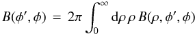 (A.3b)is the temporal correlation of the electric fields on the celestial sphere between azimuths φ′ and φ integrated over radius ρ, and
 ![Mathematical equation: \appendix \setcounter{section}{1} % subequation 2829 2 \begin{eqnarray} \label{Eq:A.3c} B(\rho,\phi^{\prime},\phi) &= &\left< \frac{1}{2} E(\rho,\phi^{\prime};t) \, E^{*}(\rho,\phi;t) \right> \, = \, \left<\frac{1}{2} \left[ E_{r}(\rho,\phi^{\prime};t) + j E_{i}(\rho,\phi^{\prime};t) \right] \left[ E_{r}(\rho,\phi;t) - j E_{i}(\rho,\phi;t) \right] \right> \nonumber \\ &= &\left[ \left<\frac{1}{2} E_{r}(\rho,\phi^{\prime};t) \, E_{r}(\rho,\phi;t)\right> + \left<\frac{1}{2} E_{i}(\rho,\phi^{\prime};t) \, E_{i}(\rho,\phi;t)\right> \right] \, + \, j \left[ -\left<\frac{1}{2} E_{r}(\rho,\phi^{\prime};t) \, E_{i}(\rho,\phi;t)\right> + \left<\frac{1}{2} E_{i}(\rho,\phi^{\prime};t) \, E_{r}(\rho,\phi;t)\right> \right] \nonumber \\ &= &\left[ B_{rr}(\rho,\phi^{\prime},\phi) + B_{ii}(\rho,\phi^{\prime},\phi) \right] \, + \, j \left[ - B_{ri}(\rho,\phi^{\prime},\phi) + B_{ir}(\rho,\phi^{\prime},\phi) \right] \, = \, B_{r}(\rho,\phi^{\prime},\phi) \, + \, j B_{i}(\rho,\phi^{\prime},\phi) \end{eqnarray}](/articles/aa/full_html/2012/05/aa18774-12/aa18774-12-eq180.png) (A.3c)is the temporal correlation of the electric fields on the celestial sphere between azimuths φ′ and φ at radius ρ. In general, B(φ′,φ) and B(ρ,φ′,φ) are complex numbers written in terms of complex electric fields. Similarly, the ( − m, − m)th POAM autocorrelation on the celestial sphere is
(A.3c)is the temporal correlation of the electric fields on the celestial sphere between azimuths φ′ and φ at radius ρ. In general, B(φ′,φ) and B(ρ,φ′,φ) are complex numbers written in terms of complex electric fields. Similarly, the ( − m, − m)th POAM autocorrelation on the celestial sphere is  (A.3d)which is obtained by replacing m → − m and exchanging φ′ ↔ φ in Eq. (A.3a). Note that B ∗ (ρ,φ′,φ) = B(ρ,φ,φ′) and B ∗ (φ′,φ) = B(φ,φ′).
As stated elsewhere, lZ = 0 when B − m, − m = Bm,m for all m. I define the quantity.
 (A.4a)where
  (A.4b)For an SAA source, the temporal statistics of Er(ρ,φ;t) and Ei(ρ,φ;t) are identical to each other. The temporal statistics of Er(ρ,φ′;t) and Ei(ρ,φ′;t) are also identical to each other, but they are not identical to the temporal statistics at (ρ,φ). Therefore, Bri(φ′,φ) = Bir(φ′,φ), Bi(φ′,φ) = 0, ΔBm = for all m, and lZ = 0. In other words, if the complex electric fields are spatially uncorrelated, their real and imaginary parts are spatially uncorrelated as well. Conversely, for a non-SAA source I find that Bri(φ′,φ) ≠ Bir(φ′,φ), Bi(φ′,φ) ≠ 0, ΔBm ≠ 0 for all m, and thus lZ ≠ 0. Q.E.D.
Appendix B: Telescope POAM autocorrelations
The (m,m)th single-telescope PSF sensitivity (Eq. (5c)) is the squared magnitude of the mth single-telescope DF sensitivity, or =  . The mth single-telescope DF sensitivity is simply the azimuthal Fourier component in the image plane of the DF, or
 ![Mathematical equation: \appendix \setcounter{section}{2} \begin{equation} \label{Eq:TelDM2} D_{m}(\rho^{\prime},\vecbf{\Omega}) \, = \, \frac{1}{2\pi} \, \int_{0}^{2\pi} \, {\rm d}\phi^{\prime} \, {\rm e}^{-j m \phi^{\prime}} \, D(\vecbf{\Omega}^{\prime},\vecbf{\Omega}) \, = \, \int {\rm d}^{2}R \, \left[ \frac{1}{2\pi} \int_{0}^{2\pi} {\rm d}\phi^{\prime} \, {\rm e}^{-jm \phi^{\prime}} \, {\rm e}^{-j2\pi \vecbf{R} \cdot \vecbf{\Omega}^{\prime}} \, \right] \, {\rm e}^{j2\pi \vecbf{R} \cdot \vecbf{\Omega}} \, s(\vecbf{R}) . \end{equation}](/articles/aa/full_html/2012/05/aa18774-12/aa18774-12-eq201.png) (B.1)The quantity in square brackets is j − mJm(2πRρ′) e − jmψ. When the aperture function is expanded into azimuthal Fourier components, I obtain
(B.1)The quantity in square brackets is j − mJm(2πRρ′) e − jmψ. When the aperture function is expanded into azimuthal Fourier components, I obtain ![Mathematical equation: \appendix \setcounter{section}{2} \begin{eqnarray} \label{Eq:TelDM3} D_{m}(\rho^{\prime},\vecbf{\Omega}) = j^{-m} \sum_{p=-\infty}^{\infty} 2\pi \int_{0}^{R_{\rm tel}} {\rm d}R \, R \, J_{m}(2\pi R \rho^{\prime}) \left[ \frac{1}{2\pi} \int_{0}^{2\pi} {\rm d}\psi \, {\rm e}^{j(p-m) \psi} {\rm e}^{j2\pi \vecbf{R} \cdot \vecbf{\Omega}} \right] s_{p}(R) . ~~~~ \end{eqnarray}](/articles/aa/full_html/2012/05/aa18774-12/aa18774-12-eq205.png) (B.2)The quantity in square brackets is jp − mJp − m(2πRρ) ej(p − m)φ. After replacing p with m − k and rearranging, the result is
(B.2)The quantity in square brackets is jp − mJp − m(2πRρ) ej(p − m)φ. After replacing p with m − k and rearranging, the result is ![Mathematical equation: \appendix \setcounter{section}{2} \begin{equation} \label{Eq:TelDM4} D_{m}(\rho^{\prime},\vecbf{\Omega}) \, = \, j^{-m} \, \sum_{k=-\infty}^{\infty} \, j^{k} \, \left[ 2\pi \, \int_{0}^{R_{\rm tel}} \, {\rm d}R \, R \, J_{m}(2\pi R \rho^{\prime}) \, s_{m-k}(R) \, J_{k}(2\pi R \rho) \right] \, {\rm e}^{-jk \phi} \, = \, j^{-m} \, \sum_{k=-\infty}^{\infty} \, j^{k} \, \mathcal{J}_{m,k}(\rho^{\prime},\rho) \, {\rm e}^{-jk \phi} . \end{equation}](/articles/aa/full_html/2012/05/aa18774-12/aa18774-12-eq211.png) (B.3)The squared magnitude of this equation is identical to Eq. (6b), which can be substituted into Eq. (5a) to give the complete (m,m)th single-telescope POAM autocorrelation densities. Q.E.D.
(B.3)The squared magnitude of this equation is identical to Eq. (6b), which can be substituted into Eq. (5a) to give the complete (m,m)th single-telescope POAM autocorrelation densities. Q.E.D.
Appendix C: Illustrative forms
To derive the first illustrative form, I change the indices k → m − p and l → m − q of Eqs. (6b) and (7). The resulting total POAM kernel becomes 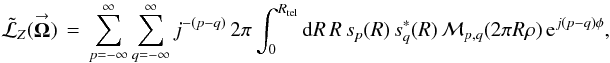 (C.1a)where
 ![Mathematical equation: \appendix \setcounter{section}{3} % subequation 3265 1 \begin{equation} \label{Eq:MPQ} \mathcal{M}_{p,q}(2\pi R \rho) \, = \, \sum_{m=-\infty}^{\infty} m \, J_{m-p}(2\pi R \rho) \, J_{m-q}(2\pi R \rho) \, = \, p \, \delta_{q,p} \, + \, \frac{1}{2} \left[ 2\pi R \rho \right] \, \delta_{q,p+1} \, + \, \frac{1}{2} \left[ 2\pi R \rho \right] \, \delta_{q,p-1} . \end{equation}](/articles/aa/full_html/2012/05/aa18774-12/aa18774-12-eq215.png) (C.1b)When Eqs. (C.1a), (b) are substituted back into Eq. (7), I obtain
(C.1b)When Eqs. (C.1a), (b) are substituted back into Eq. (7), I obtain  (C.2a)where
  (C.2b)is the integrated and squared (m,m)th component of the aperture function, the
 ![Mathematical equation: \appendix \setcounter{section}{3} % subequation 3302 2 \begin{equation} \label{Eq:Dpm} \mathcal{D}_{\mp}(\rho) \, = \, 2\pi \int_{0}^{R_{\rm tel}} {\rm d}R \, R \, \left( 2\pi R \rho \right) \, \left[ \sum_{m=-\infty}^{\infty} s_{m}(R) \, s^{*}_{m \mp 1}(R) \right] \end{equation}](/articles/aa/full_html/2012/05/aa18774-12/aa18774-12-eq218.png) (C.2c)are the aperture dipole-moment functions, and the
(C.2c)are the aperture dipole-moment functions, and the ![Mathematical equation: \appendix \setcounter{section}{3} % subequation 3302 3 \begin{equation} \label{Eq:Rancor_pm_1} \mathcal{B}_{\mp 1}(\rho) \, = \, \frac{1}{2\pi} \int_{0}^{2\pi} {\rm d}\phi \, {\rm e}^{\pm j \phi} \, B(\vecbf{\Omega}) \, = \, \frac{1}{2\pi} \int_{0}^{2\pi} {\rm d}\phi \, {\rm e}^{\pm j \phi} \left[ \sum_{n=-\infty}^{\infty} \sum_{m=-\infty}^{\infty} B_{n,m}(\rho) \, {\rm e}^{j (n-m) \phi} \right] \, = \, \sum_{n=-\infty}^{\infty} B_{n,n \pm 1}(\rho) \end{equation}](/articles/aa/full_html/2012/05/aa18774-12/aa18774-12-eq219.png) (C.2d)are the first-order source rancors (Elias 2008; Eqs. (12a), (12b)). Note that p was replaced with m so that Eqs. (C.2a), (C.2c) are consistent with the equations in Sect. 4.2. The total intensity in the image plane can be rewritten as
(C.2d)are the first-order source rancors (Elias 2008; Eqs. (12a), (12b)). Note that p was replaced with m so that Eqs. (C.2a), (C.2c) are consistent with the equations in Sect. 4.2. The total intensity in the image plane can be rewritten as ![Mathematical equation: \appendix \setcounter{section}{3} % subequation 3384 0 \begin{equation} \label{Eq:AllBTilde2} \tilde{B} \, = \, \lim_{\rho_{\rm FOV} \rightarrow \infty} \int_{\rho_{\rm FOV}} {\rm d}^{2}\Omega^{\prime} \tilde{B}(\vecbf{\Omega}^{\prime}) \, = \, \int {\rm d}^{2}\Omega \int {\rm d}^{2}R \int {\rm d}^{2}R^{\prime} \left[ \lim_{\rho_{\rm FOV} \rightarrow \infty} \int_{\rho_{\rm FOV}} {\rm d}^{2}\Omega^{\prime} {\rm e}^{-j2\pi (\vecbf{R} - \vecbf{R}^{\prime}) \cdot \vecbf{\Omega}^{\prime}} \right] {\rm e}^{j2\pi (\vecbf{R} - \vecbf{R}^{\prime}) \cdot \vecbf{\Omega}} s(\vecbf{R}) s^{*}(\vecbf{R}^{\prime}) B(\vecbf{\Omega}) . \end{equation}](/articles/aa/full_html/2012/05/aa18774-12/aa18774-12-eq220.png) (C.3a)The quantity in the square brackets approaches
(C.3a)The quantity in the square brackets approaches  , which means that
 ![Mathematical equation: \appendix \setcounter{section}{3} % subequation 3384 1 \begin{equation} \label{Eq:AllBTilde3} \tilde{B} \, \approx \, \left[ \int {\rm d}^{2}R \, S(\vecbf{R}) \right] \, \left[ \int {\rm d}^{2}\Omega \, B(\vecbf{\Omega}) \right] \, = \, S \, B , \end{equation}](/articles/aa/full_html/2012/05/aa18774-12/aa18774-12-eq222.png) (C.3b)where
(C.3b)where  . When this equation is substituted into Eq. (C.2a), I can define the aperture probabilities
  , the aperture transitional probability densities = sm(R)
  , and the celestial sphere transitional probability densities pn,n ± 1(ρ) = Bn,n ± 1(ρ)/B. Keeping in mind that ℬ-1(ρ) =
  and
and  =
=  , the result can be rearranged to obtain Eq. (8). Q.E.D.
To derive the second illustrative form, I rewrite the sum over transitional probabilities in the aperture in Eq. (8) as  (C.4a)where = (Rcosψ,Rsinψ) and
  = (Rcosψ′,Rsinψ′) (both aperture points are located in the same ring R =
  =
=  ). The quantity in parentheses is 2πδ(ψ′ − ψ), so
  (C.4b)which are the normalized first-order aperture rancor gains. Substituting Eq. (C.4b) into (C.2c), Eq. (C.2a) can be rearranged to form Eq. (9a). Q.E.D.
To derive the third illustrative form, the imaginary part of the integrand of Eq. (9a) can be simplified to ![Mathematical equation: \appendix \setcounter{section}{3} \begin{eqnarray} \label{Eq:ImPart} \mathrm{Im} \left( 2\pi R \rho \right) \left[ \frac{\mathcal{B}_{\mp 1}(\rho)}{B} \right] \left[ \frac{\mathcal{S}_{\pm 1}(R)}{S} \right] &= &\pm \, \frac{1}{2\pi} \int_{0}^{2\pi} {\rm d}\phi \, \frac{1}{2\pi} \int_{0}^{2\pi} {\rm d}\psi ~ 2\pi \left[ R \rho \sin{(\phi-\psi)} \right] \frac{B(\vecbf{\Omega})}{B} \, \frac{S(\vecbf{R})}{S} \nonumber \\ &= &\pm \frac{1}{2\pi} \int_{0}^{2\pi} {\rm d}\phi \, \frac{1}{2\pi} \int_{0}^{2\pi} {\rm d}\psi ~ 2\pi \left[ \vecbf{\Omega} \times \vecbf{R} \right] \frac{B(\vecbf{\Omega})}{B} \, \frac{S(\vecbf{R})}{S} \cdot \end{eqnarray}](/articles/aa/full_html/2012/05/aa18774-12/aa18774-12-eq240.png) (C.5)When this expression is substituted back into Eq. (9a), Eq. (10) is obtained. Q.E.D.
(C.5)When this expression is substituted back into Eq. (9a), Eq. (10) is obtained. Q.E.D.
Appendix D: Interferometer POAM autocorrelations
To prove that Eq. (11a) can be expressed in terms of a single integral over baseline for standard non-POAM interferometry analysis, I substitute = − to obtain ![Mathematical equation: \appendix \setcounter{section}{4} \begin{equation} \label{Eq:IntResponse2} \tilde{B}(\vecbf{\Omega}^{\prime}) = \int {\rm d}^{2}R \, \int_{+\vecbf{R}} {\rm d}^{2}b {\rm e}^{-j 2\pi \vecbf{b} \cdot \vecbf{\Omega}^{\prime}} s(\vecbf{R}+\vecbf{b}) s^{*}(\vecbf{R}) \mathcal{F}(\vecbf{b}) = \int {\rm d}^{2}b \, {\rm e}^{-j 2\pi \vecbf{b} \cdot \vecbf{\Omega}^{\prime}} \left[ \int {\rm d}^{2}R \, s(\vecbf{R}+\vecbf{b}) s^{*}(\vecbf{R}) \right] \mathcal{F}(\vecbf{b}) = \int {\rm d}^{2}b \, {\rm e}^{-j 2\pi \vecbf{b} \cdot \vecbf{\Omega}^{\prime}} S(\vecbf{b}) \mathcal{F}(\vecbf{b}) , ~ \end{equation}](/articles/aa/full_html/2012/05/aa18774-12/aa18774-12-eq241.png) (D.1)where
(D.1)where  is the baseline-based gain function. The
  shift in the integral can be ignored. The integral inside the square brackets must be the baseline-based gain function. Each point in the aperture function corresponds to the position of a telescope. The aperture function appears twice in the integral because there are two telescopes in a baseline. The two telescopes are separated by the baseline. Q.E.D.
To derive the (m,m)th interferometer POAM autocorrelation density, I substitute  (D.2a)into Eq. (11a) and find that
 ![Mathematical equation: \appendix \setcounter{section}{4} % subequation 3676 1 \begin{eqnarray} \label{Eq:IntResponse3} \tilde{B}(\vecbf{\Omega}^{\prime}) &= &\int {\rm d}^{2}R^{\prime} \int {\rm d}^{2}R \left[ \sum_{m=-\infty}^{\infty} j^{-m} J_{m}(2\pi R^{\prime} \rho^{\prime}) {\rm e}^{-j m (\psi^{\prime} - \phi^{\prime})} \right] \left[ \sum_{n=-\infty}^{\infty} j^{n} J_{n}(2\pi R \rho^{\prime}) {\rm e}^{j n (\psi - \phi^{\prime})} \right] \tilde{\mathcal{F}}(\vecbf{R}^{\prime},\vecbf{R}) \nonumber \\ &= &\sum_{m=-\infty}^{\infty} \sum_{n=-\infty}^{\infty} \left[ j^{-(m-n)} \int {\rm d}^{2}R^{\prime} \int {\rm d}^{2}R J_{m}(2\pi R^{\prime} \rho^{\prime}) J_{n}(2\pi R \rho^{\prime}) {\rm e}^{-j m \psi^{\prime}} {\rm e}^{j n \psi} \tilde{\mathcal{F}}(\vecbf{R}^{\prime},\vecbf{R}) \right] {\rm e}^{j (m-n) \phi^{\prime}} \nonumber \\ &= &\sum_{m=-\infty}^{\infty} \sum_{n=-\infty}^{\infty} \tilde{B}_{m,n}(\rho^{\prime}) \, {\rm e}^{j (m-n) \phi^{\prime}} . \end{eqnarray}](/articles/aa/full_html/2012/05/aa18774-12/aa18774-12-eq245.png) (D.2b)Each m = n term is identical to Eq. (12a). When Eq. (12a) is integrated over radius in the image plane, this integral
(D.2b)Each m = n term is identical to Eq. (12a). When Eq. (12a) is integrated over radius in the image plane, this integral  (D.2c)appears as one of the factors in the result. This Dirac delta function collapses the R′ integral, leaving Eq. (12b). Q.E.D.
To prove that the interferometer POAM autocorrelations of Eq. (12b) can be converted the single-telescope illustrative forms (cf. Sect. 4.2), I form the total POAM in the image plane ![Mathematical equation: \appendix \setcounter{section}{4} % subequation 3771 0 \begin{equation} \label{Eq:BTildeMMTotal2Summed} \tilde{l}_{Z} \, = \, \sum_{m=-\infty}^{\infty} m \, \tilde{p}_{m,m} \, = \, \frac{1}{\tilde{B}} \sum_{m=-\infty}^{\infty} m \, \tilde{B}_{m,m} \, = \, \frac{1}{\tilde{B}} \, 2\pi \int_{0}^{R_{int}} {\rm d}R \, R \frac{1}{2\pi} \int_{0}^{2\pi} {\rm d}\psi^{\prime} \frac{1}{2\pi} \int_{0}^{2\pi} {\rm d}\psi \left[ \sum_{m=-\infty}^{\infty} m \, {\rm e}^{-jm (\psi^{\prime} - \psi)} \right] \tilde{\mathcal{F}}(\vecbf{r},\vecbf{R}) . \end{equation}](/articles/aa/full_html/2012/05/aa18774-12/aa18774-12-eq248.png) (D.3a)The quantity in the square brackets is
(D.3a)The quantity in the square brackets is  (D.3b)which is proportional to the derivative of another delta function identity. Since
  (D.3c)Eq. (D.3a) then becomes
 ![Mathematical equation: \appendix \setcounter{section}{4} % subequation 3771 3 \begin{eqnarray} \label{Eq:Torque4} \tilde{l}_{Z} &= &-j \int {\rm d}^{2}R \left. \frac{ \partial \tilde{\mathcal{F}}(\vecbf{r},\vecbf{R}) }{ \partial \psi^{\prime} } \right|_{\psi^{\prime} = \psi} \Bigg/ \tilde{B} \, = \, -j \int {\rm d}^{2}R \, \left. \frac{\partial s(\vecbf{r})}{\partial \psi^{\prime}} \right|_{\psi^{\prime} = \psi} s^{*}(\vecbf{R}) / S \, + \, \int {\rm d}^{2}\Omega \int {\rm d}^{2}R \, \left[2\pi R \rho \sin{(\phi-\psi)}\right] \, B(\vecbf{\Omega}) \, S(\vecbf{R}) / \tilde{B} \nonumber \\ &= &\sum_{m=-\infty}^{\infty} m \, p^{a}_{m,m} \, + \, 2\pi \int {\rm d}^{2}\Omega \int {\rm d}^{2}R \, \left[ \vecbf{\Omega} \times \vecbf{R} \right] \, p(\vecbf{\Omega}) \, p^{a}(\vecbf{R}) , \end{eqnarray}](/articles/aa/full_html/2012/05/aa18774-12/aa18774-12-eq251.png) (D.3d)where the required variables and functions are defined in Appendix C. This equation is identical to the third illustrative form. The third illustrative form was derived from the other two in Appendix C, so there is no need to rederive them here. Q.E.D.
(D.3d)where the required variables and functions are defined in Appendix C. This equation is identical to the third illustrative form. The third illustrative form was derived from the other two in Appendix C, so there is no need to rederive them here. Q.E.D.
Appendix E: Interpolation with no POAM modulation
In this appendix, I assume an aperture function interpolation of the form  (E.1)where
  is the interpolation kernel,
  is the interpolated aperture coordinate, and
  = (ℛcosΨ,ℛ,sinΨ) is the real aperture coordinate. Both coordinates are in units of wavelength. This equation can be expanded into POAM components
  (E.2a)where Rlimit is the radial integration limit (Rtel for single telescopes or Rint for interferometers),
  (E.2b)is the double Fourier series expansion of the interpolation kernel, and
  (E.2c)is the POAM expansion of the non-interpolated aperture function. All of these equations have been derived using POAM calculi (Elias 2008).
By definition, a system that does not modulate the POAM spectrum means that a single input POAM state gives rise only to the same output POAM state (Elias 2008), so the interpolation kernel POAM gain must be  δn,m. The interpolation kernels that produce such POAM gains consist of the family of functions that exhibit circular symmetry, or
  (E.3)To prove this assertion, I substitute this kernel into Eq. (E.2b) and obtain
 ![Mathematical equation: \appendix \setcounter{section}{5} % subequation 3978 0 \begin{equation} \label{Eq:KernelPOAMCirc} \mathcal{K}^{-m}_{n}(R,\mathcal{R}) \, = \, \left[ \frac{1}{2\pi} \int_{0}^{2\pi} {\rm d}\chi \, {\rm e}^{-jm\chi} \, \mathcal{K}(\sqrt{R^{2}+\mathcal{R}^{2}-2R\mathcal{R}\cos{(\psi-\Psi)}}) \right] \, \left[ \frac{1}{2\pi} \int_{0}^{2\pi} {\rm d}\psi \, {\rm e}^{-j(n-m)\psi} \right] \, = \, K_{m}(R,\mathcal{R}) \, \delta_{n,m} , \end{equation}](/articles/aa/full_html/2012/05/aa18774-12/aa18774-12-eq264.png) (E.4a)which means that
(E.4a)which means that  (E.4b)I employed a change of integration variable Ψ = ψ − χ and eliminated ψ from both χ integration limits. Q.E.D.
This type of circularly symmetric interpolation kernel is often used in interferometric imaging, which is indeed fortunate. According to Eq. (E.4b), it appears that the sn(ℛ) must be calculated in order to determine the  . This procedure is unnecessarily complicated. If one substitutes Eq. (E.2c) into (E.4b), one finds that
 ![Mathematical equation: \appendix \setcounter{section}{5} \begin{equation} \label{Eq:SnTildeS} \tilde{s}_{n}(R) \, = \, \int {\rm d}^{2}\mathcal{R} \, \left[K_{n}(R,\mathcal{R}) \, {\rm e}^{-jn\Psi} \right] \, s(\vecbf{\mathcal{R}}) . \end{equation}](/articles/aa/full_html/2012/05/aa18774-12/aa18774-12-eq271.png) (E.5)In other words, the nth interpolated POAM gain can be calculated directly from the continuous or discrete aperture function and the kernel contained in the square brackets.
(E.5)In other words, the nth interpolated POAM gain can be calculated directly from the continuous or discrete aperture function and the kernel contained in the square brackets.
Appendix F: Telescope apodization in interferometers
The interferometric PSF in Eq. (14) can be expanded as a interferometric DF dual azimuthal Fourier series squared, or  (F.1)where
  is defined in Eq. (16b). Similarly, the source intensity can be expanded into its POAM correlation expansion
  (F.2)When these equations are substituted into Eq. (14), the indices rearranged, and the integral over φ performed, Eqs. (15b), (c) result. Q.E.D.
All Figures
|
Fig. 1 Schematic diagram of a single telescope looking at a source on the celestial sphere. The coordinates are indicated and described in the text of Sect. 4. The electric fields (celestial sphere and image plane) and aperture function are also presented. |
| In the text | |
|
Fig. 2 Schematic diagram of an interferometer looking at a source on the celestial sphere. The coordinates are indicated and described in the text of Sects. 4 and 5. The electric fields (celestial sphere and image plane) and aperture function are also presented. The aperture function refers to the synthesized aperture, not to the individual telescope (or pinhole) apertures that sample it. |
| In the text | |
|
Fig. 3 Holographic amplitude measurements of the EVLA antennas. The blue and red colors represent the low and high reflectivity regions. The coordinate units are wavelengths. |
| In the text | |
|
Fig. 4 Holographic phase measurements of the EVLA antennas. The yellow colors represent raised regions with respect to the fiducial dish surfaces. The rms panel deviations are ≈ 200 μm. The coordinate units are wavelengths. |
| In the text | |
|
Fig. 5 Holographic probability spectra of the EVLA antennas. The ordinates are log (base 10) probability/100% and the abscissae are POAM states. The total torque is written on each subplot. |
| In the text | |
Current usage metrics show cumulative count of Article Views (full-text article views including HTML views, PDF and ePub downloads, according to the available data) and Abstracts Views on Vision4Press platform.
Data correspond to usage on the plateform after 2015. The current usage metrics is available 48-96 hours after online publication and is updated daily on week days.
Initial download of the metrics may take a while.