| Issue |
A&A
Volume 541, May 2012
|
|
|---|---|---|
| Article Number | A94 | |
| Number of page(s) | 17 | |
| Section | Planets and planetary systems | |
| DOI | https://doi.org/10.1051/0004-6361/201118743 | |
| Published online | 04 May 2012 | |
“TNOs are Cool”: A survey of the trans-Neptunian region
VI. Herschel/PACS observations and thermal modeling of 19 classical Kuiper belt objects⋆
1
Max-Planck-Institut für extraterrestrische Physik,
Postfach 1312, Giessenbachstr.,
85741
Garching,
Germany
e-mail: This email address is being protected from spambots. You need JavaScript enabled to view it.
2 Konkoly Observatory of the Hungarian Academy of Sciences,
1525 Budapest, PO Box 67, Hungary
3
Deutsches Zentrum für Luft- und Raumfahrt e.V., Institute of
Planetary Research, Rutherfordstr.
2, 12489
Berlin,
Germany
4
LESIA-Observatoire de Paris, CNRS, UPMC Univ. Paris 06, Univ. Paris-Diderot,
France
5
Stewart Observatory, The University of Arizona,
Tucson
AZ
85721,
USA
6
SRON LEA/HIFI ICC, Postbus 800, 9700AV
Groningen, The
Netherlands
7
UNS-CNRS-Observatoire de la Côte d’Azur, Laboratoire Cassiopée,
BP 4229,
06304
Nice Cedex 04,
France
8
Center for Geophysics of the University of Coimbra,
Av. Dr. Dias da
Silva, 3000-134
Coimbra,
Portugal
9
Astronomical Observatory of the University of Coimbra,
Almas de Freire,
3040-04
Coimbra,
Portugal
10
Univ. Paris Diderot, Sorbonne Paris Cité, 4 rue Elsa Morante,
75205
Paris,
France
11
Laboratoire d’Astrophysique de Marseille, CNRS &
Université de Provence, 38 rue
Frédéric Joliot-Curie, 13388
Marseille Cedex 13,
France
12
Instituto de Astrofísica de Andalucía (CSIC),
Camino Bajo de Huétor
50, 18008
Granada,
Spain
13
INAF – Osservatorio Astronomico di Roma, via di Frascati, 33,
00040
Monte Porzio Catone,
Italy
14
INAF – Osservatorio Astronomico di Capodimonte, Salita Moiariello
16, 80131
Napoli,
Italy
15
University of Maryland, College Park, MD
20742,
USA
16
IMCCE, Observatoire de Paris, 77 Av. Denfert-Rochereau, 75014
Paris,
France
17
Max-Planck-Institut für Sonnensystemforschung,
Max-Planck-Straße
2, 37191
Katlenburg-Lindau,
Germany
Received: 25 December 2011
Accepted: 6 March 2012
Abstract
Context. Trans-Neptunian objects (TNO) represent the leftovers of the formation of the solar system. Their physical properties provide constraints to the models of formation and evolution of the various dynamical classes of objects in the outer solar system.
Aims. Based on a sample of 19 classical TNOs we determine radiometric sizes, geometric albedos and beaming parameters. Our sample is composed of both dynamically hot and cold classicals. We study the correlations of diameter and albedo of these two subsamples with each other and with orbital parameters, spectral slopes and colors.
Methods. We have done three-band photometric observations with Herschel/PACS and we use a consistent method for data reduction and aperture photometry of this sample to obtain monochromatic flux densities at 70.0, 100.0 and 160.0 μm. Additionally, we use Spitzer/MIPS flux densities at 23.68 and 71.42 μm when available, and we present new Spitzer flux densities of eight targets. We derive diameters and albedos with the near-Earth asteroid thermal model (NEATM). As auxiliary data we use reexamined absolute visual magnitudes from the literature and data bases, part of which have been obtained by ground based programs in support of our Herschel key program.
Results. We have determined for the first time radiometric sizes and albedos of eight classical TNOs, and refined previous size and albedo estimates or limits of 11 other classicals. The new size estimates of 2002 MS4 and 120347 Salacia indicate that they are among the 10 largest TNOs known. Our new results confirm the recent findings that there are very diverse albedos among the classical TNOs and that cold classicals possess a high average albedo (0.17 ± 0.04). Diameters of classical TNOs strongly correlate with orbital inclination in our sample. We also determine the bulk densities of six binary TNOs.
Key words: Kuiper belt: general / infrared: planetary systems / techniques: photometric
Herschel is an ESA space observatory with science instruments provided by European-led Principal Investigator consortia and with important participation from NASA.
© ESO, 2012
1. Introduction
The physical properties of small solar system bodies offer constraints on theories of the formation and evolution of the planets. Trans-Neptunian objects (TNO), also known as Kuiper belt objects (KBO), represent the leftovers from the formation period of the outer solar system (Morbidelli et al. 2008), and they are analogues to the parent bodies of dust in debris disks around other stars (Wyatt 2008; Moro-Martín et al. 2008, and references therein).
In addition to Pluto more than 1400 TNOs have been discovered since the first KBO in 1992 (Jewitt & Luu 1993), and the current discovery rate is 10 to 40 new TNOs/year. The dynamical classification is based on the current short-term dynamics. We use the classification of Gladman (Gladman et al. 2008, 10 Myr time-scale): classical TNOs are those non-resonant TNOs which do not belong to any other TNO class. The classical TNOs are further divided into the main classical belt, the inner belt (a < 39.4 AU) and the outer belt (a > 48.4 AU). The eccentricity limit for classicals is e < 0.24, beyond which targets are classified as detached or scattered objects. The classification scheme of the Deep Eplictic Survey team (DES, Elliot et al. 2005) differs from the Gladman system in terms of the boundary of classical and scattered objects, which do not show a clear demarcation in their orbital parameters. Some of the classicals in the Gladman system are scattered-near or scattered-extended in the DES system. Another division is made in the inclination/eccentricity space. Although there is no dynamical separation, there seems to be two distinct but partly overlapping inclination distributions with the low-i “cold” classicals, limited to the main classical belt, showing different average albedo (Grundy et al. 2005; Brucker et al. 2009), color (Trujillo & Brown 2002), luminosity function (Fraser et al. 2010), and frequency of binary systems (Noll et al. 2008) than the high-i “hot” classicals, which has a wider inclination distribution. Furthermore, models based on recent surveys suggest that there is considerable sub-structure within the main classical belt (Petit et al. 2011). To explain these differences more quantitative data on physical size and surface composition are needed.
The physical characterization of TNOs has been limited by their large distance and relatively small sizes. Accurate albedos help to correctly interpret spectra and are needed to find correlations in the albedo-size-color-orbital parameters space that trace dynamical and collisional history. The determination of the size frequency distribution (SFD) of TNOs provides one constraint to formation models and gives the total mass. The SFD of large bodies is dominated by accretion processes and they hold information about the angular momentum of the pre-solar nebula whereas bodies smaller than 50 to 100 km are the result of collisional evolution (Petit et al. 2008). The SFD can be estimated via the luminosity function (LF), but this size distribution also depends on assumptions made about surface properties such as albedo. Consequently, ambiguities in the size distributions derived from the LFs of various dynamical classes are one significant reason why there is a wide uncertainty in the total TNO mass estimate ranging from 0.01 MEarth (Bernstein et al. 2004) to 0.2 MEarth (Chiang et al. 1999). Among the formation models of our solar system the “Nice” family of models have been successful in explaining the orbits of planets and the formation of the Kuiper belt (Tsiganis et al. 2005; Levison et al. 2008), although they have difficulties in explaining some of the details of the cold and hot distributions and the origin of the two sub-populations (e.g. Fraser et al. 2010; Petit et al. 2011; Batygin et al. 2011).
Only a few largest TNOs have optical size estimates based on direct imaging and assumptions about the limb darkening function (e.g. Quaoar, Fraser & Brown 2010). The combination of optical and thermal infrared observations gives both sizes and geometric albedos, but requires thermal modeling. Earlier results from Spitzer and Herschel have shown the usefulness of this method (e.g. Stansberry et al. 2008; Müller et al. 2010) and significantly changed the size and albedo estimates of several TNOs compared to those obtained by using an assumed albedo.
In this work we present new radiometric diameters and geometric albedos for 19 classical TNOs. Half of them have no previously published observations in the wavelength regime used in this work. Those which have been observed before by Spitzer now have more complete sampling of their spectral energy distributions (SEDs) close to the thermal peak. The new estimates of the 19 targets are based on observations performed with the ESA Herschel Space Observatory (Pilbratt et al. 2010) and its Photodetector Array Camera and Spectrometer (PACS; Poglitsch et al. 2010). Other Herschel results for TNOs have been presented by Müller et al. (2010), Lellouch et al. (2010) and Lim et al. (2010). New estimates of 18 Plutinos are presented in Mommert et al. (2012) and of 15 scattered disc and detached objects in Santos-Sanz et al. (2012).
This paper is organized in the following way. We describe our target sample in Sect. 2.1, Herschel observations in Sect. 2.2 and Herschel data reduction in Sect. 2.3. New or re-analyzed flux densities from Spitzer are presented in Sect. 2.4. As auxiliary data we use absolute V-band magnitudes (Sect. 2.5), which we have adopted from other works or data bases taking into account the factors relevant to their uncertainty estimates. Thermal modeling is described in Sect. 3 and the results for individual targets in Sect. 4. In Sect. 5 we discuss sample properties of our sample and of all classicals with radiometric diameters and geometric albedos as well as correlations (Sect. 5.1) and the bulk densities of binaries (Sect. 5.2). Finally, the conclusions are in Sect. 6.
2. Observations and data reduction
Our sample of 19 TNOs has been observed as part of the Herschel key program “TNOs are Cool” (Müller et al. 2009) mainly between February and November 2010 by the photometry sub-instrument of PACS in the wavelength range 60–210 μm.
2.1. Target sample
The target sample consists of both dynamically cold and hot classicals (Table 1). We use a cut-off limit of i = 4.5° in illustrating the two subsamples. Another typical value used in the literature is i = 5°. The inclination limit is lower for large objects (Petit et al. 2011) which have a higher probability of belonging to the hot population. Targets 119951 (2002 KX14), 120181 (2003 UR292) and 78799 (2002 XW93) are in the inner classical belt and are therefore considered to belong to the low-inclination tail of the hot population. The latter two would be Centaurs in the DES system and all targets in Table 1 with i > 15° would belong to the scattered-extended class of DES.
The median absolute V-magnitudes (HV, see Sect. 2.5) of our sample are 6.1 mag for the cold sub-sample and 5.3 mag for the hot one. Levison & Stern (2001) found that bright classicals have systematically higher inclinations than fainter ones. This trend is seen among our targets (see Sect. 5.1.3). Another known population characteristics is the lack of a clear color demarcation line at i ≈ 5° (Peixinho et al. 2008), which is absent also from our sample of 10 targets with known colors.
Target sample.
Individual observations of the sample of 19 TNOs by Herschel/PACS.
2.2. Herschel observations
PACS is an imaging dual band photometer with a rectangular field of view of 1.75′ × 3.5′ with full sampling of the 3.5 m-telescope’s point-spread function (PSF). The two detectors are bolometer arrays, the short-wavelength one has 64 × 32 pixels and the long-wavelength one 32 × 16 pixels. In addition, the short-wavelength array has a filter wheel to select between two bands: 60−85 μm or 85−125 μm, whereas the long-wavelength band is 125−210 μm. In the PACS photometric system these bands have been assigned the reference wavelengths 70.0 μm, 100.0 μm and 160.0 μm and they have the names “blue”, “green” and “red”. Both bolometers are read-out at 40 Hz continuously and binned by a factor of four on-board.
We specified the PACS observation requests (AOR) using the scan-map Astronomical Observation Template (AOT) in HSpot, a tool provided by the Herschel Science Ground Segment Consortium. The scan-map mode was selected due to its better overall performance compared to the point-source mode (Müller et al. 2010). In this mode the pointing of the telescope is slewed at a constant speed over parallel lines, or “legs”. We used 10 scan legs in each AOR, separated by 4″. The length of each leg was 3.0′, except for Altjira where it was 2.5′, and the slewing speed was 20″ s-1. Each one of these maps was repeated from two to five times.
To choose the number of repetitions, i.e. the duration of observations, for our targets we used the Standard Thermal Model (see Sect. 3) to predict their flux densities in the PACS bands. Based on earlier Spitzer work (Stansberry et al. 2008) we adopted a geometric albedo of 0.08 and a beaming parameter of 1.25 for observation planning purposes. The predicted thermal fluxes depend on the sizes, which are connected to the assumed geometric albedo and the absolute V-magnitudes via Eq. (3). In some cases the absolute magnitudes used for planning purposes are quite different (by up to 0.8 mag) from those used for modeling our data as more recent and accurate visible photometry was taken into account (see Sect. 2.5).
The PACS scan-map AOR allows the selection of either the blue or green channel; the red channel data are taken simultaneously whichever of those is chosen. The sensitivity of the blue channel is usually limited by instrumental noise, while the red channel is confusion-noise limited (PACS AOT release note 2010). The sensitivity in the green channel can be dominated by either source, depending on the depth and the region of the sky of the observation. For a given channel selection (blue or green) we grouped pairs of AORs, with scan orientations of 70° and 110° with respect to the detector array, in order to make optimal use of the rectangular shape of the detector. Thus, during a single visit of a target we grouped 4 AORs to be observed in sequence: two AORs in different scan directions and this repeated for the second channel selection.
The timing of the observations, i.e. the selection of the visibility window, has been optimized to utilize the lowest far-infrared confusion noise circumstances (Kiss et al. 2005) such that the estimated signal-to-noise ratio due to confusion noise has its maximum in the green channel. Each target was visited twice with similar AORs repeated in both visits for the purpose of background subtraction. The timing of the second visit was calculated such that the target has moved 30−50″ between the visits so that the target position during the second visit is within the high-coverage area of the map from the first visit. Thus, we can determine the background for the two source positions.
The observational details are listed in Table 2. All of the targets observed had predicted astrometric 3σ uncertainties less than 10″ at the time of the Herschel observations (David Trilling, priv. comm.).
2.3. Data reduction
The data reduction from level 0 (raw data) to level 2 (maps) was done using Herschel Interactive Processing Environment (HIPE1) with modified scan-map pipeline scripts optimized for the “TNOs are Cool” key program. The individual maps (see Fig. 1 for examples) from the same epoch and channel are mosaicked, and background-matching and source-stacking techniques are applied. The two visits are combined (Fig. 2), in each of the three bands, and the target with a known apparent motion is located at the center region of these maps. The detector pixel sizes are 3.2″ × 3.2″ in the blue and green channels, and 6.4″ × 6.4″ in the red channel whereas the pixel sizes in the maps produced by this data reduction are 1.1″/1.4″/2.1″ in the blue/green/red maps, respectively. A detailed description of the data reduction in the key program is given in Kiss et al. (in prep.).
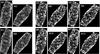 |
Fig. 1 Individual maps of 120347 Salacia. Each map is the product of one observation (AOR). The first row (M1-M6) is from the first visit and the second row (M7-M12) from the follow-on visit. The first two columns (M1-M2, M7-M8) are observations in the 100 μm or “green” channel and the others in the 160 μm or “red” channel. The two scan angles are 110° (odd-numbered maps) and 70°. The source is clearly seen in the map center in the green channel whereas the red channel is more affected by background sources and confusion noise. Orientation: north is up and east is to the left. |
Once the target is identified we measure the flux densities at the photocenter position using DAOPHOT routines (Stetson 1987) for aperture photometry. We make a correction for the encircled energy fraction of a point source (PACS photometer PSF 2010) for each aperture used. We try to choose the optimum aperture radius in the plateau of stability of the growth-curves, which is typically 1.0−1.25 times the full-width-half-maximum of the PSF (5.2″/7.7″/12.0″ in the blue/green/red bands, respectively). The median aperture radius for targets in the “TNOs are Cool” program is 5 pixels in the final maps (pixel sizes 1.1″/1.4″/2.1″ in the blue/green/red maps). For the uncertainty estimation of the flux density we implant 200 artificial sources in the map in a region close to the source (<50″) excluding the target itself. A detailed description of how aperture photometry is implemented in our program is given in Santos-Sanz et al. (2012).
In order to obtain monochromatic flux density values of targets having a SED different from the default one color corrections are needed. In the photometric system of the PACS instrument flux density is defined to be the flux density that a source with a flat spectrum (λFλ = const., where λ is the wavelength and Fλ is the monochromatic flux) would have at the PACS reference wavelengths (Poglitsch et al. 2010). Instead of the flat default spectrum we use a cool black body distribution to calculate correction coefficients for each PACS band. The filter transmission and bolometer response curves needed for this calculation are available from HIPE, and we take as black body temperature the disk averaged day-side temperature calculated iteratively for each target ( , using STM assumptions from Sect. 3, the Lambertian emission model and the sub-solar temperature from Eq. (2)). This calculation yields on the average 0.982/0.986/1.011 for the blue/green/red channels, respectively, with small variation among the targets of our sample.
The absolute flux density calibration of PACS is based on standard stars and large main belt asteroids and has the uncertainties of 3%/3%/5% for the blue/green/red bands (PACS photometer – Point Source Flux Calibration 2011). We have taken these uncertainties into account in the PACS flux densities used in the modeling, although their contribution to the total uncertainty is small compared to the signal-to-noise ratio of our observations.
The color corrected flux densities are given in Table 3. They were determined from the combined maps of two visits, in total 4 AORs for the blue and green channels and 8 AORs for the red. The only exceptions are 19521 Chaos and 90568 (2004 GV9), whose one map was excluded from our analysis due to a problem in obtaining reliable photometry from those observations. The uncertainties include the photometric 1σ and absolute calibration 1σ uncertainties. 17 targets were detected in at least one PACS channel. The upper limits are the 1σ noise levels of the maps, including both the instrumental noise and residuals from the eliminated infrared background confusion noise. 79360 Sila has a flux density which is lower by a factor of three in the red channel than the one published by Müller et al. (2010). We have re-analyzed this earlier chopped/nodded observation using the latest knowledge on calibration and data reduction and found no significant change in the flux density values. As speculated in Müller et al. (2010) the 2009 single-visit Herschel observation was most probably contaminated by a background source.
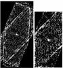 |
Fig. 2 Combined maps of 120347 Salacia from the individual maps (Fig. 1) in the green (left) and red channels. Orientation: north is up and east is to the left. |
Color corrected Herschel flux densities of the sample of 19 classical TNOs from coadded images of two visits.
2.4. Complementary Spitzer observations
About 75 TNOs and Centaurs in the “TNOs are Cool” program were also observed by the Spitzer Space Telescope (Werner et al. 2004) using the Multiband Imaging Photometer for Spitzer (MIPS; Rieke et al. 2004). 43 targets were detected at a useful signal-to-noise ratio in both the 24 μm and 70 μm bands of that instrument. As was done for our Herschel program, many of the Spitzer observations utilized multiple AORs for a single target, with the visits timed to allow subtraction of background confusion. The MIPS 24 μm band, when combined with 70−160 μm data, can provide very strong constraints on the temperature of the warmest regions of a TNO.
The absolute calibration, photometric methods and color corrections for the MIPS data are described in 31, 24 and 83. Nominal calibration uncertaintes are 2% and 4% in the 24 μm and 70 μm bands respectively. To allow for additional uncertainties that may be caused by the sky-subtraction process, application of color corrections, and the faintness of TNOs relative to the MIPS stellar calibrators, we adopt uncertainties of 3% and 6% as has been done previously for MIPS TNO data (e.g. Stansberry et al. 2008; Brucker et al. 2009). The effective monochromatic wavelengths of the two MIPS bands we use are 23.68 μm and 71.42 μm. With an aperture of 0.85 m the telescope-limited spatial resolution is 6″ and 18″ in the two bands.
Spitzer flux densities of 13 targets overlapping our classical TNO sample are given in Table 4. The new and re-analyzed flux densities are based on re-reduction of the data using updated ephemeris positions. They sometimes differ by 10″ or more from those used to point Spitzer. The ephemeris information is used in the reduction of the raw 70 μm data, for generating the sky background images, and for accurate placement of photometric apertures. This is especially important for the Classical TNOs which are among the faintest objects observed by Spitzer. Results for four targets are previously unpublished: 275809 (2001 QY297), 79360 Sila, 88611 Teharonhiawako, and 19521 Chaos. As a result of the reprocessing of the data, the fluxes for 119951 (2002 KX14), 148780 Altjira, 2001 KA77 and 2002 MS4 differ from those published in Brucker et al. (2009) and Stansberry et al. (2008).
The 70 μm bands of PACS and MIPS are overlapping and the flux density values agree typically within ± 5% for the six targets observed by both instruments with SNR ≳ 2.
Complementary Spitzer observations.
Overview of optical auxiliary data.
2.5. Optical photometry
The averages of V-band or R-band absolute magnitude values available in the literature are given in Table 1. The most reliable way of determining them is to observe a target at multiple phase angles and over a time span enough to determine lightcurve properties, but such complete data are available only for 119951 (2002 KX14) in our sample. For all other targets assumptions about the phase behavior have been made due to the lack of coverage in the range of phase angles.
The IAU (H, G) magnitude system for photometric phase curve corrections (Bowell et al. 1989), which has been adopted in some references, is known to fail in the case of many TNOs (Belskaya et al. 2008). Due to the lack of a better system we prefer linear methods as a first approximation since TNOs have steep phase curves which do not deviate from a linear one in the limited phase angle range usually available for TNO observations. The opposition surge of very small phase angles (α ≲ 0.2°, Belskaya et al. 2008) has not been observed for any of our 19 targets due to the lack of observations at such small phase angles. All of our Herschel and Spitzer observations are limited to the range 1.0° < α < 2.1°.
We have used the linear method (HV = V − 5log (rΔ) − βα, where V is the apparent V-magnitude in the Johnson-Coussins or the Bessel V-band, and other symbols are as in Table 2, and β is the linearity coefficient) to calculate the HV values from individual V-magnitudes given in the references (see Table 5) for 2001 XR254, 275809 (2001 QY297), 79360 Sila, 88611 Teharonhiawako, 148780 Altjira and 19521 Chaos. In order to be consistent with most of the HV values in the literature we have adopted β = 0.14 ± 0.03 calculated from Sheppard & Jewitt (2002). The effect of slightly different values of β or assumptions of its composite value used in previous works is usually negligible compared to uncertainties caused by lightcurve variability (an exception is 90568 (2004 GV9)).
For five targets with no other sources available we take the absolute magnitudes in the R-band (HR in Table 5) from the Minor Planet Center and calculate their standard deviation, since the number of V-band observations for these targets is very low, and use the average (V − R) color index for classical TNOs 0.59 ± 0.15 (Hainaut & Delsanti 2002) to derive HV. While the MPC is mainly used for astrometry and the magnitudes are considered to be inaccurate by some works (e.g. Benecchi et al. 2011; Romanishin & Tegler 2005), for the five targets we use the average of 9 to 16 R-band observations and adopt the average R-band phase coefficient βR = 0.12 (calculated from Belskaya et al. 2008).
The absolute V-magnitudes used as input in our analysis (the “Corrected HV” column in Table 5) take into account additional uncertainties from known or assumed variability in HV. The amplitude, the period and the time of zero phase of the lightcurves of three hot classicals (145452 (2005 RN43), 90568 (2004 GV9) and 120347 Salacia) are available in the literature, but even for these three targets the uncertainty in the lightcurve period is too large to be used for exact phasing with Herschel observations. The lightcurve amplitude or amplitude limit is known for half of our targets and for them we add 88% of the half of the peak-to-peak amplitude (1σ i.e. 68% of the values of a sinusoid are within this range) quadratically to the uncertainty of HV. According to a study of a sample of 74 TNOs from various dynamical classes (Duffard et al. 2009) 70% of TNOs have a peak-to-peak amplitude ≲ 0.2 mag, thus we quadratically add 0.09 mag to the uncertainty of HV for those targets in our sample for which lightcurve information is not available.
3. Thermal modeling
The combination of observations from thermal-infrared and optical wavelengths allows us to estimate various physical properties via thermal modeling. For a given temperature distribution the disk-integrated thermal emission F observed at wavelength λ is 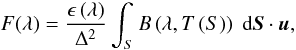 (1)where ϵ is the emissivity, Δ the observer-target distance, B(λ,T) Planck’s radiation law for black bodies,
  the temperature distribution on the surface S and u the unit directional vector toward the observer from the surface element dS. The temperature distribution of an airless body depends on physical parameters such as diameter, albedo, thermal inertia, and surface roughness.
There are three basic types of models to predict the emission of an asteroid with a given size and albedo assuming an equilibrium between insolation and re-emitted thermal radiation: the Standard Thermal Model (STM), the Fast-rotating Isothermal Latitude thermal model (Veeder et al. 1989), and the thermophysical models (starting from Matson 1971; e.g. Spencer et al. 1989; Lagerros 1996). While originally developed for asteroids in the mid-IR wavelengths these models are applicable for TNOs, whose thermal peak is in the far-IR.
The STM (cf. Lebofsky et al. 1986, and references therein) assumes a smooth, spherical asteroid, which is not rotating and/or has zero thermal inertia, and is observed at zero phase angle. The subsolar temperature TSS is ![Mathematical equation: \begin{equation} \label{Tss} T_{\mathrm{SS}} = \left[\frac{ \left(1-A\right)S_{\sun}}{\epsilon \eta \sigma r^2} \right]^{\frac{1}{4}}, \end{equation}](/articles/aa/full_html/2012/05/aa18743-11/aa18743-11-eq279.png) (2)where A is the Bond albedo, S⊙ is the solar constant, η is the beaming factor, σ is the Stefan-Boltzmann constant and r is the heliocentric distance. In the STM ϵ does not depend on wavelength. The beaming factor η adjusts the subsolar temperature. The canonical value η = 0.756 is based on calibrations using the largest few main belt asteroids. The STM assumes an average linear infrared phase coefficient of 0.01 mag/degree based on observations of main belt asteroids.
(2)where A is the Bond albedo, S⊙ is the solar constant, η is the beaming factor, σ is the Stefan-Boltzmann constant and r is the heliocentric distance. In the STM ϵ does not depend on wavelength. The beaming factor η adjusts the subsolar temperature. The canonical value η = 0.756 is based on calibrations using the largest few main belt asteroids. The STM assumes an average linear infrared phase coefficient of 0.01 mag/degree based on observations of main belt asteroids.
In this work we use the Near-Earth Asteroid Thermal Model NEATM (Harris 1998). The difference to the STM is that in the NEATM η is fitted with the data instead of using a single canonical value. For rough surfaces η takes into account the fact that points on the surface S radiate their heat preferentially in the sunward direction. High values (η > 1) lead to a reduction of the model surface temperature, mimicking the effect of high thermal inertia, whereas lower values are a result of surface roughness. Furthermore, the phase angle α is taken into account by calculating the thermal flux an observer would detect from the illuminated part of S assuming a Lambertian emission model and no emission from the non-illuminated side.
Whenever data quality permits we treat η as a free fitting parameter. However, in some cases of poor data quality this method leads to η values which are too high or too low and therefore unphysical. In these cases we fix it to a canonical value of η = 1.20 ± 0.35 derived by Stansberry et al. (2008) from Spitzer observations of TNOs. The physical range of η values is determined by using NEATM as explained in Mommert et al. (2012) to be 0.6 ≤ η ≤ 2.6.
Throughout this work we assume the surface emissivity ϵ = 0.9, which is based on laboratory measurements of silicate powder up to a wavelength of 22 μm (Hovis & Callahan 1966) and a usual approximation for small bodies in the solar system. At far-IR wavelengths the emissivity of asteroids may be decreasing as a function of wavelength (Müller & Lagerros 1998) from 24 to 160 μm, but the amount depends on individual target properties. Thus, a constant value is assumed for simplicity. The variation of emissivity of icy surfaces as a function of wavelength could in principle provide hints about surface composition. H2O ice has an emissivity close to one with small variations (Schmitt et al. 1998) whereas other ices may show a stronger wavelength dependence (e.g. Stansberry et al. 1996). Near-IR spectroscopic surface studies have been done for five of our targets but none of them show a reliable detection of ices, even though many dynamically hot classicals are known to have ice signatures in their spectra (Barucci et al. 2011).
For the Bond albedo we assume that A ≈ AV since the V-band is close to the peak of the solar spectrum. The underlying assumption is that the Bond albedo is not strongly varying across the relevant solar spectral range of reflected light. The Bond albedo is connected to the geometric albedo via AV = pVq, where q is the phase integral and pV the geometric albedo in V-band. Instead of the canonical value of q = 0.39 (Bowell et al. 1989) we have adopted q = 0.336pV + 0.479 (Brucker et al. 2009), which they used for a Spitzer study of classical TNOs. From the definition of the absolute magnitude of asteroids we have: 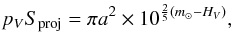 (3)where Sproj is the area projected toward the observer, a is the distance of one astronomical unit, m⊙ is the apparent V-magnitude of the Sun, and HV is the absolute V-magnitude of the asteroid. We use m⊙ = (− 26.76 ± 0.02) mag (Bessell et al. 1998; Hayes 1985). An error of 0.02 mag in HV means a relative error of 1.8% in the product (3).
We find the free parameters pV,  and η in a weighted least-squares sense by minimizing the cost function
 ![Mathematical equation: \begin{equation} \chi_{\nu}^2=\frac{1}{\nu} \sum_{i=1}^{N} \frac{\left[ F \left( \lambda_i \right) - F_{\mathrm{model}} \left( \lambda_i \right)\right]^2}{\sigma_i^2}, \label{chi2} \end{equation}](/articles/aa/full_html/2012/05/aa18743-11/aa18743-11-eq301.png) (4)where ν is the number of degrees of freedom, N is the number of data points in the far-infrared wavelengths,
(4)where ν is the number of degrees of freedom, N is the number of data points in the far-infrared wavelengths,  is the observed flux density at wavelength λi with uncertainty σi, and Fmodel is the modeled emission spectrum. When only upper flux density limits are available, they are treated as having zero flux density with a 1σ uncertainty equal to the upper limit flux density uncertainty (0 ± σ). The cost function (4) does not follow the χ2 statistical distribution since in a non-linear fit the residuals are not normally distributed even if the flux densities had normally distributed uncertainties.
3.1. Error estimates
The error estimates of the geometric albedo, the diameter and the beaming parameter are determined by a Monte Carlo method described in 55. We generate 500 sets of synthetic flux densities normally distributed around the observed flux densities with the same standard deviations as the observations. Similarly, a set of normally distributed HV values is generated. For those targets whose χ2 ≫ 1 we do a rescaling of the errorbars of the flux densities before applying the Monte Carlo error estimation as described in Santos-Sanz et al. (2012) and illustrated in Mommert et al. (2012).
The NEATM model gives us the effective diameter of a spherical target. 70−80% of TNOs are known to be MacLaurin spheroids with an axial ratio of 1.15 (Duffard et al. 2009; Thirouin et al. 2010). When the projected surface has the shape of an ellipse instead of a circle, then this ellipse will emit more flux than the corresponding circular disk which has the same surface because the Sun is seen at higher elevations from a larger portion of the ellipsoid than on the sphere. Therefore, the NEATM diameters may be slightly overestimated. Based on studies of model accuracy (e.g. Harris 2006) we adopt uncertainties of 5% in the diameter estimates and 10% in the pV estimates to account for systematic model errors when NEATM is applied at small phase angles.
4. Results of individual targets
In this Section we give the results of model fits using the NEATM to determine the area-equivalent diameters (see Sect. 3) as well as geometric albedos and beaming factors. We note that our observations did not spatially resolve binary systems, we therefore find area-equivalent diameters of the entire system rather than component diameters; this will be further discussed in Sect. 5.2.
In cases where also Spitzer/MIPS data are available for a target we determine the free parameters for both PACS only and the combined data sets. The solutions are given in Table 6. A floating-η solution is only adopted if its χ2 is not much greater than unity. The exact limit depends on the number of data points. For N = 5 this limit is χ2 ≲ 1.7. For the PACS-only data set we may adopt floating-η solutions only if there are no upper-limit data points. 138537 (2000 OK67) has only upper limits from PACS, therefore only the solution using combined data is shown. 2001 RZ143 has five data points, three of which are upper limits. The PACS flux density at 70 μm is approximately a factor of three higher than the MIPS upper limit (see Tables 3 and 4). For this target we adopt the model solution determined without the MIPS 70 μm channel. The best solution for each target is shown in Fig. 3.
The radiometric diameters determined with data from the two instruments are on the average close to the corresponding results using PACS data alone, but there are some significant differences as well, most notably 275809 (2001 QY297) and 2002 KW14. The former has a PACS-only solution, which is within the error bars of the green and red channel data points, but above the PACS blue channel data point. When the two upper limits from MIPS are added in the analysis the model solution is at a lower flux level below the PACS green channel data point but compatible with the other data (see Fig. 3). 2002 KW14 has upper limits in the PACS green and red channels as well as in the MIPS 24 μm channel. Without this upper limit in the shortest wavelength the PACS-only solution is at higher flux levels in short wavelengths and gives a lower flux at long wavelengths.
When choosing the preferred solution we are comparing two fits with different numbers of data points used, therefore in this comparison we calculate χ2 for the PACS-only solution using the same data points as for the combined solution taking into account the different observing geometries during Herschel and Spitzer observations. In all cases where MIPS data is available the solution based on the combined data from the two instruments is the preferred one.
2002 GV31 is the only non-detection by both PACS and MIPS in our sample of 19 targets. The astrometric 3σ uncertainty at the time of the PACS observation was <4″ (semimajor axis of the confidence ellipsoid2), which is well within the high-coverage area of our maps.
Solutions for radiometric diameters and geometric albedos (see text for explanations).
The error bars from the Monte Carlo error estimation method may sometimes be too optimistic compared to the accuracy of optical data and the model uncertainty of NEATM (see Sect. 3). We check that the uncertainty of geometric albedo is not better than the uncertainty implied by the optical constraint (Eq. (3)) due to uncertainties in HV and m⊙. The lower pV uncertainty of four targets is limited by this (see Table 6).
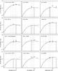 |
Fig. 3 Adopted model solutions from Table 6. The black data points are from PACS (70, 100 and 160 μm) and the gray points are from MIPS (24 and 71 μm) normalized to the geometry of Herschel observations by calculating the NEATM solution (for given D, pV and η) at both the epochs of the Herschel and Spitzer observations and using their ratio as a correction factor. |
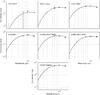 |
Fig. 3 continued. |
5. Discussion
Our new size and geometric albedo estimates improve the accuracy of previous estimates of almost all the targets with existing results or limits (Table 7). Two thirds of our targets have higher albedos (Table 6) than the 0.08 used in the planning of these observations, which has lead to the lower than expected SNRs and several upper limit flux densities (Table 3). Previous results from Spitzer are generally compatible with our new estimates. However, two targets are significantly different: 119951 (2002 KX14) and 2001 KA77, whose solutions are compatible with the optical constraint (Eq. (3)), but the new estimate has a large diameter and low albedo (target 119951) instead of a small diameter and high albedo, or vice versa (target 2001 KA77). It can be noted that there is a significant difference in the re-processed Spitzer flux densities at 70 μm compared to the previously published values (see Table 4), which together with the PACS 100 μm data can explain the significant change in the diameter and geometric albedo estimates. Our new estimates for 148780 Altjira differ from the previous upper and lower limits based on Spitzer data alone (Table 7). This change can be explained by the addition of the 70 μm and 100 μm PACS data points (Table 3) to the earlier MIPS 24 μm value and the MIPS 70 μm upper flux density limit (Table 4).
Adopted physical properties in comparison with previous works.
The diameter estimates in our sample are ranging from 100 km of 120181 (2003 UR292) up to 930 km of 2002 MS4, which is larger than previously estimated for it. 2002 MS4 and 120347 Salacia are among the ten largest TNOs with sizes similar to those of 50000 Quaoar and 90482 Orcus. The size distribution of hot classicals in our sample is wider than that of the cold classicals, which are limited to diameters of 100−350 km (Fig. 4). The diameters of eight hot classicals from literature data (Table 7) are within the same size range as the hot classicals in our sample. The cumulative size distribution of this extended set of 20 hot classicals (Fig. 5) shows two regimes of a power law distribution with a turning point between 500 and 700 km. The slope of the cumulative distribution N(>D) ∝ D−q is q ≈ 1.4 for the 100 < D < 600 km (N = 11) objects. There are not enough targets for a reliable slope determination in the D > 600 km regime. The size distribution is an important property in understanding the processes of planet formation. Several works have derived it from the LF using simplifying assumptions about common albedo and distance. Fraser et al. (2010) reported a slope of the differential size distribution of 2.8 ± 1.0 for a dynamically hot TNO population (38 AU < heliocentric distance < 55 AU and i > 5°). Our q + 1 based on a small sample of measured diameters of intermediate-size hot classicals is compatible with this literature value. The high-q tail at D > 650 km in Fig. 5 indicates a change of slope when the population transitions from a primordial one to a collisionally relaxed population. Based on LF estimates, this change in slope for the whole TNO population was expected at 200−300 km (Kenyon et al. 2008; based on data from Bernstein et al. 2004) or at somewhat larger diameters (Petit et al. 2006). For Plutinos a change to a steeper slope occurs at 450 km (Mommert et al. 2012).
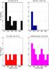 |
Fig. 4 Distribution of diameters from this work (upper left), the cold classicals of this work (upper right), the hot classicals of this work (lower left), and all hot classicals including literature results from Table 7 (lower right). The last plot includes only dynamically hot classicals. The bin size is 100 km. |
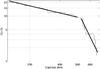 |
Fig. 5 Cumulative size distribution of dynamically hot classicals from this work and literature (Table 7). The power law has a change between 500 and 700 km. The intermediate size classicals have a slope parameter of q = 1.4. |
The dynamically cold and hot sub-populations are showing different geometric albedo distributions (Fig. 6) with the dynamically cold objects having higher geometric albedos in a narrower distribution. The average geometric albedo of the six cold classicals is 0.17 ± 0.04 (un-weighted average and standard deviation). The highest-albedo object is 88611 Teharonhiawako with pV = 0.22, or possibly 2002 GV31 with the lower limit of 0.22. These findings are compatible with the conclusions of Brucker et al. (2009) based on Spitzer data that cold classicals have a high albedo, although we do not confirm their extreme geometric albedo of 0.6 for 119951 (2002 KX14).
The darkest object in our sample is the dynamically hot target 78799 (2002 XW93) with a geometric albedo of 0.038. The highest-albedo hot classicals are found in the low-i part of the sub-sample (see Fig. 7): 138537 (2000 OK67) at i = 4.9° has pV = 0.20 and the inner belt target 120181 (2003 UR292) has a geometric albedo of 0.16. The 12 hot classicals in our sample have, on the average, lower albedos than the cold ones: pV = 0.09 ± 0.05. The average of the combined hot classical sub-population of this work and literature is 0.11 ± 0.04 if 55636 (2002 TX300) is excluded.
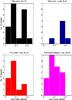 |
Fig. 6 Distribution of geometric albedos from this work (upper left), the cold classicals of this work (upper right), the hot classicals of this work (lower left), and all hot classicals including literature results from Table 7 (lower right). The bin size is 0.05. The Haumea family member 55636 (2002 TX300) with pV = 0.88 is beyond the horizontal scale. |
From the floating-η solutions of eight targets with data from both instruments included in the fitted solution (see Table 6 and Sect. 4) we have the average η = 1.47 ± 0.43 (un-weighted). Most of these eight targets have η > 1 implying a noticeable amount of surface thermal inertia. It should be noted, though, that inferences about surface roughness and thermal conductivity would require more accurate knowledge of the spin axis orientation and spin period of these targets. Our average η is consistent with our default value of 1.20 ± 0.35 for fixed η fits. For comparison with other dynamical classes, the average beaming parameter of seven Plutinos is  (Mommert et al. 2012) and of seven scattered and detached objects η = 1.14 ± 0.15 (Santos-Sanz et al. 2012). The difference of using a fixed-η = 1.47 instead of fixed-η = 1.20 is that diameters would increase, on the average, by 10% and geometric albedos decrease by 16%. These changes are within the average relative uncertainties (19% in diameter and 57% in geometric albedo) of the fixed-η solutions.
5.1. Correlations
We ran a Spearman rank correlation test (Spearman 1904) to look for possible correlations between the geometric albedo pV, diameter D, orbital elements (inclination i, eccentricity e, semimajor axis a, perihelion distance q), beaming parameter η, visible spectral slope, as well as B − V, V − R and V − I colors3. The Spearman correlation is a distribution-free test less sensitive to outliers than some other more common methods (e.g. Pearson correlation). We use a modified form of the test, which takes into account asymmetric error bars and corrects the significance for small numbers statistics. The details of our method are described in 64 and Santos-Sanz et al. (2012). The significance P of a correlation is the probability of getting a higher or equal correlation coefficient value −1 ≤ ρ ≤ 1 if no correlation existed on the parent population, from which we extracted the sample. Therefore, the smaller the P the more unlikely would be to observe a ρ ≠ 0 if it was indeed equal to zero, i.e. the greater the confidence on the presence of a correlation is. The 99.7% confidence interval (3σ), or better, corresponds to P = 0.003, or smaller. We consider a “strong correlation” to have |ρ| ≥ 0.6, and a “moderate correlation” to have 0.3 ≤ |ρ| < 0.6. Selected results from our correlation analysis are presented in Table 8 and discussed in the following subsections.
5.1.1. Correlations with diameter
We detect a strong size-inclination correlation in our target sample (see Fig. 7 and Table 8). When literature targets, all of whom are dynamically hot, are included in the analysis we get a correlation of similar strength. Previously this presumable trend has been extrapolated from the correlation between intrinsic brightness and inclination (Levison & Stern 2001). We see this strong size-inclination correlation also among the hot classicals sub-sample, but not among our cold classicals where we are limited by the small sample size.
Other orbital parameters do not correlate with size. We find no correlation between size and colors, or spectral slopes, nor between size and the beaming parameter η. The possible correlation between size and geometric albedo is discussed in Sect. 5.1.2.
5.1.2. Correlations with geometric albedo
We find evidence for an anti-correlation between diameter and geometric albedo, both in our sample and when combined with other published data of classical TNOs (see Fig. 8 and Table 8). Other dynamical populations with accurately measured diameters/albedos show a different behavior: there is no such correlation seen among the Plutinos (Mommert et al. 2012) and a combined sample of 15 scattered-disc and detached objects show a positive correlation between diameter and geometric albedo at 2.9σ level (Santos-Sanz et al. 2012).
As it might be suggested visually by the distribution of diameters of classical TNOs (see Figs. 4 and 8), we have analyzed the possibility of having two groups with different size-albedo behaviors, separating in size at D ≈ 500 km regardless of their dynamical cold/hot membership. We have found no statistical evidence for it.
With our method of accounting for error bars, which tend to “degrade” the correlation values, geometric albedo does not correlate with HV, orbital parameters, spectral slopes, colors, nor beaming parameters η. Also when the literature targets are added we find no evidence of correlations.
5.1.3. Other correlations
The known correlations between surface color/spectral slope and orbital inclination (Trujillo & Brown 2002; Hainaut & Delsanti 2002), and between intrinsic brightness and inclination (Levison & Stern 2001), usually interpreted as a size-inclination correlation, might lead us to conclude there was a consequent color/slope-size correlation. Our analysis with measured diameters does not show a correlation neither with spectral slope nor visible colors, as one might expect. Note, however, that we do not possess information on the surface colors/slopes of ~1/2 of our targets (~1/3 when complemented with other published data) leading to the non-detection of the color/slope-inclination trend, which is known to exist among classicals. Thus, a more complete set of color/slope data would be required for our targets. Only when combining the hot sub-sample from this work and literature we see a non-significant anti-correlation between slope and inclination (see Table 8). We do not find any correlations of the B − V, V − R and V − I colors with other parameters.
The apparent HV vs i anti-correlation in our target sample mentioned in Sect. 2.1 is almost significant (2.7σ) for our hot sub-population (see Table 8).
Selected correlation results (see text).
5.2. Binaries
Binary systems are of particular scientific interest because they provide unique constraints on the elusive bulk composition, whereas all other observational constraints of the composition only pertain to the surface of the object. The sizes of binaries can be constrained based on the relative brightness difference of the primary and the secondary components, but only if suitable assumptions about the relative geometric albedo are made. Alternatively, geometric albedos can be constrained under certain assumptions about the relative sizes. The ranges given in the literature are usually based on the following assumptions: i) the primary and secondary objects are spherical, ii) the primary and secondary have equal albedos, and iii) objects have densities within a limited assumed range.
Six of our targets are binaries with known total mass m and brightness difference between the two components ΔV (see Table 9). Assuming the two components to have identical albedos, the latter can be converted into an area ratio and, assuming spherical shape, a diameter ratio k = D2/D1 (with component diameters D1 and D2). Component diameters follow from the measured NEATM diameter D (see Table 6) and D2/D1:  (since D is the area-equivalent system diameter). This leads to a “volumetric diameter”
  . The mass densities
  are given in Table 9. Within the uncertainties, the measured bulk densities scatter around roughly 1 g cm-3, consistent with a bulk composition dominated by water ice, as expected for objects in the outer solar system. Significant mass contributions from heavier materials, such as silicates, are not excluded however, and would have to be compensated by significant amounts of macroporosity. The largest object, 120347 Salacia, has a bulk density >1 g cm-3. This could indicate a lower amount of macroporosity for this object, which is subject to significantly larger gravitational self-compaction than our other binary targets.
6. Conclusions
The number of classical TNOs with both the size and the geometric albedo measured radiometrically is increased by eight from 22 to 30. Four other targets, which previously had estimated size ranges from the analysis of binary systems, now have more accurate size estimates. The number of targets observed and analysed within the “TNOs are Cool” program (Müller et al. 2010; Lellouch et al. 2010; Lim et al. 2010; Santos-Sanz et al. 2012; Mommert et al. 2012) is increased by 18 and the observation of 79360 Sila disturbed by a background source in Müller et al. (2010) has been re-observed and analyzed. Furthermore, three targets which earlier had upper and lower limits only based on Spitzer data alone (148780 Altjira, 138537 (2000 OK67) and 2001 RZ143) now have accurately estimated diameters and albedos. The new Altjira solution is outside of the previous limits based on Spitzer data alone. The three PACS data points near the thermal peak are providing reliable diameter/albedo solutions, but in some cases adding Spitzer data, especially the 24 μm data point in the lower-wavelength regime, constrains the solution and allows smaller error bars and more reliable estimates of the beaming parameter. Compared to previous works the size estimates of 119951 (2002 KX14), and 2002 MS4 have increased. 2002 MS4 (934 km) is similar in size to 50000 Quaoar and the refined size of 120347 Salacia (901 km) is similar to that of 90482 Orcus. We find a diameter for 2001 KA77, which is approximately half of the previous estimate (Brucker et al. 2009), and a geometric albedo approximately 4 times higher. The largest change in estimated geometric albedo is with 119951 (2002 KX14) from 0.60 to 0.097.
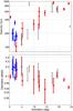 |
Fig. 7 Radiometric diameter as well as geometric albedo vs inclination. The cold classicals of our sample are marked with blue squares, hot classicals with red crosses and hot classicals from literature with gray points. The high-albedo target 55636 (2002 TX300) is beyond the scale. |
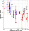 |
Fig. 8 Geometric albedo vs radiometric diameter (blue triangles = cold classicals, red crosses = hot classicals from our sample, gray = other hot classicals from literature, see Table 7). |
The main conclusions based on accurately measured classical TNOs are:
-
1.
There is a large diversity of objects’ diameters and geometricalbedos among classical TNOs.
-
2.
The dynamically cold targets have higher (average 0.17 ± 0.04) and differently distributed albedos than the dynamically hot targets (0.09 ± 0.05) in our sample. When extended by seven hot classicals from literature the average is 0.11 ± 0.04.
-
3.
Diameters of classical TNOs strongly correlate with orbital inclination in the sample of targets, whose size and geometric albedo have been accurately measured, i.e. low inclination objects are smaller. We find no clear evidence of an albedo-inclination trend.
-
4.
Our data suggests that geometric albedos of classical TNOs anti-correlate with diameter, i.e. smaller objects possess higher albedos.
-
5.
Our data does not show evidence for correlations between surface colors, or spectral slope, of classical TNOs and their diameters nor with their albedos.
-
6.
We are limited by the small sample size of radiometrically measured accurate diameters/albedos of dynamically cold classicals (N = 6) finding no statistical evidences for any correlations.
-
7.
The cumulative size distribution of hot classicals based on the sample of measured sizes in the range of diameters between 100 and 600 km (N = 11) has a slope of q ≈ 1.4.
-
8.
We determine the bulk densities of six classicals. They scatter around ~1 g cm-3. The high-mass object 120347 Salacia has a density of
 g cm-3.
New density estimates for binaries.
Data presented in this paper were analysed using “HIPE”, a joint development by the Herschel Science Ground Segment Consortium, consisting of ESA, the NASA Herschel Science Center, and the HIFI, PACS and SPIRE consortia members, see http://herschel.esac.esa.int/DpHipeContributors.shtml
Asteroids Dynamic Site by A. Milani, Z. Knezevic, O. Arratia et al., URL: http://hamilton.dm.unipi.it/astdys/, accessed August 2011, calculations based on the OrbFit software.
From the Minor Bodies in the Outer solar system data base, URL: http://www.eso.org/~ohainaut/MBOSS, accessed Nov. 2011.
Acknowledgments
We thank Chemeda Ejeta for his work in the dynamical classification of the targets of the “TNOs are Cool” program. We acknowledge the helpful efforts of David Trilling in the early planning of this program. Part of this work was supported by the German DLR project numbers 50 OR 1108, 50 OR 0903, 50 OR 0904 and 50OFO 0903. M. Mommert acknowledges support trough the DFG Special Priority Program 1385. C. Kiss and A. Pal acknowledge the support of the Bolyai Research Fellowship of the Hungarian Academy of Sciences. J. Stansberry acknowledges support by NASA through an award issued by JPL/Caltech. R. Duffard acknowledges financial support from the MICINN (contract Ramón y Cajal). P. Santos-Sanz would like to acknowledge financial support by the Centre National de la Recherche Scientifique (CNRS). J.L.O. acknowledges support from spanish grants AYA2008-06202-C03-01, P07-FQM-02998 and European FEDER funds.
References
- Altenhoff, W. J., Bertoldi, F., & Menten, K. M. 2004, A&A, 415, 771 [Google Scholar]
- Barucci, M. A., Romon, J., Doressoundiram, A., & Tholen, D. J. 2000, AJ, 120, 496 [NASA ADS] [CrossRef] [Google Scholar]
- Barucci, M. A., Alvarez-Candal, A., Merlin, F., et al. 2011, Icarus, 214, 297 [NASA ADS] [CrossRef] [Google Scholar]
- Batygin, K., Brown, M. E., & Fraser, W. C. 2011, ApJ, 738, 13 [NASA ADS] [CrossRef] [Google Scholar]
- Belskaya, I. N., Levasseur-Regourd, A.-C., Shkuratov, Y. G., & Muinonen, K., in The Solar System Beyond Neptune, ed. M. A. Barucci, H. Boehnhardt, D. P. Cruikshank, & A. Morbidelli, 115 [Google Scholar]
- Benecchi, S. D., Noll, K. S., Grundy, W. M., et al. 2009, Icarus, 200, 292 [NASA ADS] [CrossRef] [Google Scholar]
- Benecchi, S. D., Noll, K. S., Stephens, D. C., et al. 2011, Icarus, 213, 693 [NASA ADS] [CrossRef] [Google Scholar]
- Bernstein, G. M., Trilling, D. E., & Allen, R. L. 2004, AJ, 128, 1364 [NASA ADS] [CrossRef] [Google Scholar]
- Bessell, M. S., Castelli, F., & Plez, B. 1998, A&A, 333, 231 [NASA ADS] [Google Scholar]
- Boehnhardt, H., Tozzi, G. P., & Birkle, K. 2001, A&A, 378, 653 [NASA ADS] [CrossRef] [EDP Sciences] [Google Scholar]
- Bowell, E., Hapke, B., Domingue, D., et al. 1989, in Asteroids II (University of Arizona Press) [Google Scholar]
- Brucker, M. J., Grundy, W. M., Stansberry, J. A., et al. 2009, Icarus, 201, 284 [NASA ADS] [CrossRef] [Google Scholar]
- Chiang, E. I., & Brown, M. E. 1999, AJ, 118, 1411 [NASA ADS] [CrossRef] [Google Scholar]
- Davies, J. K., Green, S., McBride, N., et al. 2000, Icarus, 146, 253 [NASA ADS] [CrossRef] [Google Scholar]
- Delsanti, A. C., Böhnhardt, H., Barrera, L., et al. 2001, A&A, 380, 347 [NASA ADS] [CrossRef] [EDP Sciences] [Google Scholar]
- DeMeo, F. E., Fornasier, S., Barucci, M. A., et al. 2009, A&A, 493, 283 [NASA ADS] [CrossRef] [EDP Sciences] [Google Scholar]
- Duffard, R., Ortiz, J. L., Thirouin, A., et al. 2009, A&A, 505, 1283 [NASA ADS] [CrossRef] [EDP Sciences] [Google Scholar]
- Doressoundiram, A., Peixinho, N., de Berg, C., et al. 2002, AJ, 124, 2279 [NASA ADS] [CrossRef] [Google Scholar]
- Doressoundiram, A., Peixinho, N., Doucet, C., et al. 2005, Icarus, 174, 90 [NASA ADS] [CrossRef] [Google Scholar]
- Doressoundiram, A., Peixinho, N., Moullet, A., et al. 2007, AJ, 134, 2186 [NASA ADS] [CrossRef] [Google Scholar]
- Dotto, E., Perna, D., Barucci, M. A., et al. 2008, A&A, 490, 829 [NASA ADS] [CrossRef] [EDP Sciences] [Google Scholar]
- Elliot, J. L., Kern, S. D., Clancy, K. B., et al. 2005, AJ, 129, 1117 [NASA ADS] [CrossRef] [Google Scholar]
- Elliot, J. L., Person, M. J., Zuluaga, C. A., et al. 2010, Nature, 465, 897 [NASA ADS] [CrossRef] [PubMed] [Google Scholar]
- Engelbracht, C. W., Blaylock, M., Su, K. Y. L., et al. 2007, PASP, 119, 994 [NASA ADS] [CrossRef] [Google Scholar]
- Fornasier, S., Barucci, M. A., de Bergh, C., et al. 2009, A&A, 508, 457 [NASA ADS] [CrossRef] [EDP Sciences] [Google Scholar]
- Fraser, W. C., & Brown, M. E. 2010, ApJ, 714, 1547 [Google Scholar]
- Fraser, W. C., Brown, M. E., & Schwamb, M. E. 2010, Icarus, 210, 944 [NASA ADS] [CrossRef] [Google Scholar]
- Fulchignoni, M., Belskaya, I., Barucci, M. A., et al. 2008, in The Solar System Beyond Neptune, ed. M. A. Barucci, H. Boehnhardt, D. P. Cruikshank, & A. Morbidelli, 181 [Google Scholar]
- Giorgini, J. D., Yeomans, D. K., Chamberlin, A. B., et al. 1996, BAAS, 28, 1158 [NASA ADS] [Google Scholar]
- Gladman, B., Marsden, B. G., & VanLaerhoven, Ch. 2008, in The Solar System Beyond Neptune, ed. M. A. Barucci, H. Boehnhardt, D. P. Cruikshank, A. Morbidelli, 43 [Google Scholar]
- Gordon, K. D., Engelbracht, C. W., & Fadda, D. 2007, PASP, 119, 1019 [NASA ADS] [CrossRef] [Google Scholar]
- Grundy, W. M., Noll, K. S., & Stephens, D. C. 2005, Icarus, 176, 184 [NASA ADS] [CrossRef] [Google Scholar]
- Grundy, W. M., Noll, K. S., Buie, M. W., et al. 2009, Icarus, 200, 627 [NASA ADS] [CrossRef] [Google Scholar]
- Grundy, W. M., Noll, K. S., Nimmo, F., et al. 2011, Icarus, 213, 678 [NASA ADS] [CrossRef] [Google Scholar]
- Grundy, W. M., Benecchi, S. D., Rabinowitz, D. L., et al. 2012, Icarus, submitted [Google Scholar]
- Hainaut, O., & Delsanti, A. 2002, A&A, 389, 641, updated data base URL: http://www.eso.org/~ohainaut/MBOSS/, accessed July 2011 [NASA ADS] [CrossRef] [EDP Sciences] [Google Scholar]
- Harris, A. W. 1998, Icarus, 131, 291 [NASA ADS] [CrossRef] [EDP Sciences] [Google Scholar]
- Harris, A. W. 2006, in Asteroids, Comets, Meteors, ed. D. Lazzaro, S. Ferraz-Mello, & J. A. Fernández, Proc. IAU Symp., 229, 2005 [Google Scholar]
- Hayes, D. S. 1985, in IAU Symp. 111, ed. D. S. Hayes, et al., 225 [Google Scholar]
- Hovis, W. A., & Callahan, W. R. 1966, J. Opt. Soc. Amer., 56, 639 [Google Scholar]
- Jewitt, D., & Luu, J. 1993, Nature, 362, 730 [NASA ADS] [CrossRef] [Google Scholar]
- Kenyon, S. J., Bromley, B. C., O’Brien, D. P., & Davis, D. R. 2008, in The Solar System Beyond Neptune, ed. M. A. Barucci, H. Boehnhardt, D. P. Cruikshank, & A. Morbidelli, 293 [Google Scholar]
- Kiss, Cs., Klaas, U., & Lemke, D. 2005, A&A, 430, 343 [NASA ADS] [CrossRef] [EDP Sciences] [Google Scholar]
- Lagerros, J. S. V. 1996, A&A, 310, 1011 [NASA ADS] [Google Scholar]
- Lebofsky, L. A., & Spencer, J. R. 1989, in Asteroids II, ed. R. P. Binzel, T. Gehrels, & M. S. Matthews (Arizona University Press), 128 [Google Scholar]
- Lebofsky, L. A., Sykes, M. V., Tedesco, E. F., et al. 1986, Icarus, 68, 239 [NASA ADS] [CrossRef] [Google Scholar]
- Lellouch, E., Kiss, Cs., Santos-Sanz, P., et al. 2010, A&A, 518, L147 [NASA ADS] [CrossRef] [EDP Sciences] [Google Scholar]
- Levison, H. F., & Stern, S. A. 2001, AJ, 121, 1730 [NASA ADS] [CrossRef] [Google Scholar]
- Levison, H. F., Morbidelli, A., VanLaerhoven, Ch., et al. 2008, Icarus, 196, 258 [NASA ADS] [CrossRef] [Google Scholar]
- Lim, T. L., Stansberry, J., Müller, Th., et al. 2010, A&A, 518, L148 [Google Scholar]
- Matson, D. L., 1971, Ph.D. Thesis, California Institute of Technology [Google Scholar]
- Mommert, M., Harris, A. W., Kiss, C., et al. 2012, A&A, 541, A93 [NASA ADS] [CrossRef] [EDP Sciences] [Google Scholar]
- Morbidelli, A., Levison, H. F., & Gomes, R., 2008, in The Solar System Beyond Neptune, ed. M. A. Barucci, H. Boehnhardt, D. P. Cruikshank, & A. Morbidelli, 275 [Google Scholar]
- Moro-Martín, A., Wyatt, M. C., Malhotra, R., & Trilling, D. E. 2008, in The Solar System Beyond Neptune, ed. M. A. Barucci, H. Boehnhardt, D. P. Cruikshank, & A. Morbidelli, 465 [Google Scholar]
- Mueller, M., Delbo, M., Hora, J. L., et al. 2011, AJ, 141, 109 [NASA ADS] [CrossRef] [Google Scholar]
- Müller, T. G., & Lagerros, J. S. V. 1998, A&A, 338, 340 [NASA ADS] [Google Scholar]
- Müller, T. G., Lellouch, E., Böhnhardt, H., et al. 2009, Earth Moon and Planets, 105, 209 [CrossRef] [Google Scholar]
- Müller, Th., Lellouch, E., Stansberry, J., et al. 2010, A&A, 518, L146 [NASA ADS] [CrossRef] [EDP Sciences] [Google Scholar]
- Noll, K. S., Grundy, W. M., Stephens, D. C., et al. 2008, Icarus, 194, 758 [NASA ADS] [CrossRef] [Google Scholar]
- Osip, D. J., Kern, S. D., & Elliot, J. L. 2003, Earth, Moon, Planets, 92, 409 [Google Scholar]
- PACS AOT Release Note: PACS Photometer Point/Compact Source Mode 2010, PICC-ME-TN-036, Version 2.0, custodian Th. Müller, URL: http://herschel.esac.esa.int/twiki/bin/view/Public/PacsCalibrationWeb [Google Scholar]
- PACS photometer – Point Source Flux Calibration 2011, PICC-ME-TN-037, Version 1.0, URL: http://herschel.esac.esa.int/twiki/bin/view/ Public/PacsCalibrationWeb [Google Scholar]
- PACS photometer point spread function 2010, PICC-ME-TN-033, Version 1.01, custodian D. Lutz, http://herschel.esac.esa.int/twiki/bin/view/ Public/PacsCalibrationWeb [Google Scholar]
- Peixinho, N., Boehnhardt, H., Belskaya, I., et al. 2004, Icarus, 170, 153 [NASA ADS] [CrossRef] [Google Scholar]
- Peixinho, N., Lacerda, P., & Jewitt, D. 2008, AJ, 136, 1837 [NASA ADS] [CrossRef] [Google Scholar]
- Perna, D., Barucci, M. A., & Fornasier, S. 2010, A&A, 510, A53 [NASA ADS] [CrossRef] [EDP Sciences] [Google Scholar]
- Petit, J.-M., Holman, M. J., Gladman, B., et al. 2006, MNRAS, 365, 429 [NASA ADS] [CrossRef] [Google Scholar]
- Petit, J.-M., Kavelaars, J. J., Gladman, B., & Loredo, T. 2008, in The Solar System Beyond Neptune, ed. M. A. Barucci, H. Boehnhardt, D. P. Cruikshank, & A. Morbidelli, 71 [Google Scholar]
- Petit, J.-M., Kavelaars, J. J., Gladman, B., et al. 2011, AJ, 142, 142 [Google Scholar]
- Pilbratt, G. L., Riedinger, J. R., & Passvogel, T. 2010, A&A, 518, L1 [CrossRef] [EDP Sciences] [Google Scholar]
- Poglitsch, A., Waelkens, C., Geis, N., et al. 2010, A&A, 518, L2 [NASA ADS] [CrossRef] [EDP Sciences] [Google Scholar]
- Rabinowitz, D. L., Schaefer, B. E., & Tourtellotte, S. W. 2007, AJ, 133, 26 [NASA ADS] [CrossRef] [Google Scholar]
- Rieke, G. H., Young, E. T., Engelbracht, C. W., et al. 2004, ApJS, 154, 25 [NASA ADS] [CrossRef] [Google Scholar]
- Romanishin, W., & Tegler, S. C. 2005, Icarus, 179, 523 [NASA ADS] [CrossRef] [Google Scholar]
- Santos-Sanz, P., Ortiz, J. L., Barrera, L., & Boehnhardt, H. 2009, A&A, 494, 693 [NASA ADS] [CrossRef] [EDP Sciences] [Google Scholar]
- Santos-Sanz, P., Lellouch, E., Fornasier, S., et al. 2012, A&A, 541, A92 [NASA ADS] [CrossRef] [EDP Sciences] [Google Scholar]
- Schmitt, B., Quirico, E., Trotta, F., & Grundy, W. M. 1998, in solar system Ices, Based on reviews presented at the international symposium “Solar system ices” held in Toulouse, France, on March 27−30, 1995, ed. B. Schmitt, C. de Bergh, & M. Festou (Dordrecht Kluwer Academic Publishers), Astrophys. Space Sci. Lib. (ASSL) Ser., 227, 199 [Google Scholar]
- Sheppard, S. S. 2007, AJ, 134, 787 [NASA ADS] [CrossRef] [Google Scholar]
- Sheppard, S. S., & Jewitt, D. C. 2002, AJ, 124, 1757 [NASA ADS] [CrossRef] [Google Scholar]
- Spearman, C. 1904, Am. J. Psychol., 57, 72 [CrossRef] [Google Scholar]
- Spencer, J. R., Lebofsky, L. A., & Sykes, M. V. 1989, Icarus, 78, 337 [NASA ADS] [CrossRef] [Google Scholar]
- Stansberry, J. A., Pisano, D. J., & Yelle, R. V. 1996, Planet. Space Sci., 44, 945 [NASA ADS] [CrossRef] [Google Scholar]
- Stansberry, J., Gordon, K. D., Bhattacharya, B., et al. 2007, PASP, 119, 1038 [NASA ADS] [CrossRef] [Google Scholar]
- Stansberry, J., Grundy, W., Brown, M., et al. 2008, in The Solar System Beyond Neptune, ed. M. A. Barucci, H. Boehnhardt, D. P. Cruikshank, & A. Morbidelli, 161 [Google Scholar]
- Stansberry, J. A., Grundy, W. G., Müller, M., et al. 2012, Icarus, accepted, DOI:10.1016/j.icarus.2012.03.029 [Google Scholar]
- Stetson, P. B. 1987, PASP, 99, 191 [NASA ADS] [CrossRef] [Google Scholar]
- Tegler, S. C., & Romanishin, W. 2000, Nature, 407, 979 [NASA ADS] [CrossRef] [PubMed] [Google Scholar]
- Thirouin, A., Ortiz, J. L., & Duffard, R. 2010, A&A, 522, A93 [NASA ADS] [CrossRef] [EDP Sciences] [Google Scholar]
- Thirouin, A., Ortiz, J. L., Campo Bagatin, A., et al. 2012, MNRAS, submitted [Google Scholar]
- Trujillo, C. A., & Brown, M. E. 2002, ApJ, 566, L125 [NASA ADS] [CrossRef] [Google Scholar]
- Tsiganis, K., Gomes, R., Morbidelli, A., & Levison, H. F. 2005, Nature, 435, 459 [NASA ADS] [CrossRef] [PubMed] [Google Scholar]
- Veeder, G. J., Hanner, M. S., & Matson, D. L. 1989, AJ, 97, 1211 [NASA ADS] [CrossRef] [PubMed] [Google Scholar]
- Werner, M. W., Roellig, T. L., Low, F. J., et al. 2004, ApJS, 154, 1 [Google Scholar]
- Wyatt, M. C. 2008, ARA&A, 46, 339 [NASA ADS] [CrossRef] [Google Scholar]
All Tables
Color corrected Herschel flux densities of the sample of 19 classical TNOs from coadded images of two visits.
Solutions for radiometric diameters and geometric albedos (see text for explanations).
All Figures
|
Fig. 1 Individual maps of 120347 Salacia. Each map is the product of one observation (AOR). The first row (M1-M6) is from the first visit and the second row (M7-M12) from the follow-on visit. The first two columns (M1-M2, M7-M8) are observations in the 100 μm or “green” channel and the others in the 160 μm or “red” channel. The two scan angles are 110° (odd-numbered maps) and 70°. The source is clearly seen in the map center in the green channel whereas the red channel is more affected by background sources and confusion noise. Orientation: north is up and east is to the left. |
| In the text | |
|
Fig. 2 Combined maps of 120347 Salacia from the individual maps (Fig. 1) in the green (left) and red channels. Orientation: north is up and east is to the left. |
| In the text | |
|
Fig. 3 Adopted model solutions from Table 6. The black data points are from PACS (70, 100 and 160 μm) and the gray points are from MIPS (24 and 71 μm) normalized to the geometry of Herschel observations by calculating the NEATM solution (for given D, pV and η) at both the epochs of the Herschel and Spitzer observations and using their ratio as a correction factor. |
| In the text | |
|
Fig. 3 continued. |
| In the text | |
|
Fig. 4 Distribution of diameters from this work (upper left), the cold classicals of this work (upper right), the hot classicals of this work (lower left), and all hot classicals including literature results from Table 7 (lower right). The last plot includes only dynamically hot classicals. The bin size is 100 km. |
| In the text | |
|
Fig. 5 Cumulative size distribution of dynamically hot classicals from this work and literature (Table 7). The power law has a change between 500 and 700 km. The intermediate size classicals have a slope parameter of q = 1.4. |
| In the text | |
|
Fig. 6 Distribution of geometric albedos from this work (upper left), the cold classicals of this work (upper right), the hot classicals of this work (lower left), and all hot classicals including literature results from Table 7 (lower right). The bin size is 0.05. The Haumea family member 55636 (2002 TX300) with pV = 0.88 is beyond the horizontal scale. |
| In the text | |
|
Fig. 7 Radiometric diameter as well as geometric albedo vs inclination. The cold classicals of our sample are marked with blue squares, hot classicals with red crosses and hot classicals from literature with gray points. The high-albedo target 55636 (2002 TX300) is beyond the scale. |
| In the text | |
|
Fig. 8 Geometric albedo vs radiometric diameter (blue triangles = cold classicals, red crosses = hot classicals from our sample, gray = other hot classicals from literature, see Table 7). |
| In the text | |
Current usage metrics show cumulative count of Article Views (full-text article views including HTML views, PDF and ePub downloads, according to the available data) and Abstracts Views on Vision4Press platform.
Data correspond to usage on the plateform after 2015. The current usage metrics is available 48-96 hours after online publication and is updated daily on week days.
Initial download of the metrics may take a while.