© ESO, 2012

1. Introduction

Short bursts with a duration of less than 2 s represent about 25% of the BATSE sample (Kouveliotou et al. 1993) but had to wait until 2005 (i.e. eight years after long bursts) to enter the afterglow era (Gehrels et al. 2005; Fox et al. 2005; Hjorth et al. 2005; Berger et al. 2005). This is due to two reasons: (i) short bursts tend to emit less photons because of harder spectra and lower fluences (Kouveliotou et al. 1993), which makes their localization more difficult; (ii) they have fainter afterglows, which are harder to detect. Following the discovery of the first afterglows, it appeared that the nature of the host galaxy, the location of the afterglow, and the absence of a supernova imprint in the visible light curve (even when the host is located at a redshift below 0.5) were indicative of progenitors that were different from those of long bursts (Gehrels et al. 2005; Fox et al. 2005; Soderberg et al. 2006). Several short burts are clearly associated to elliptical galaxies (Bloom & Prochaska 2006; Berger 2009) while others with accurate positions appear to have no coincident hosts, which clearly excludes progenitors belonging to the young population and favors merger scenarios involving compact objects (Narayan et al. 1992; Mochkovitch et al. 1993; Ruffert & Janka 1999; Belczynski et al. 2006).

About 40% of the short bursts have no detectable afterglows after about 1000 s while the other 60% (Sakamoto & Gehrels 2009) have long-lasting afterglows comparable to those of long bursts (see the review on short bursts by Nakar 2007, and references therein). If short bursts indeed result from the merging of two compact objects, the kick received when the black hole or neutron star components formed in past supernova explosions (Hobbs et al. 2005; Belczynski et al. 2006) can allow the system to reach the low-density outskirts of the host galaxy (or even to leave the galaxy) before coalescence occurs. This can naturally explains why some afterglows are so dim or have no coincident host (the observational data presented in Troja et al. (2008), show that the galactocentric offset of short bursts is on average much larger than for long bursts).

The direct and simple connection between duration and progenitor class became fuzzier when it was found that in some bursts an initial short duration spike is followed by a soft tail lasting several tens of seconds (Barthelmy et al. 2005; Villasenor et al. 2005; Norris & Bonnell 2006). It was then suggested (Zhang 2006; Gehrels et al. 2006) to introduce a new terminology that would distinguish type-I bursts resulting from mergers and type-II events coming from collapsars. In the absence of a detected afterglow that can help to relate the burst to either the old or young stellar population, a vanishing spectral lag (for both the spike and the extended emission) has been proposed as an indicator for a type-I identification (Gehrels et al. 2006).

GRB 080503 belongs to the class of short bursts with extended emission. The extended emission ended with a steep decay that was not immediately followed by a standard afterglow component. A peculiar feature in GRB 080503 is that after remaining undetected for about one day, it showed a spectacular rebrightening (both in X-rays and the visible), which could be followed for five days in the visible. Perley et al. (2009) described in great detail the multi-wavelength data they collected for this event and discussed different possibilities that could account for the late rebrightening: (i) a delayed rise of the afterglow due to an extremely low density of the surrounding medium; (ii) the presence of a density clump in the burst environment; (iii) an off-axis jet that becomes visible when relativistic beaming has been reduced by deceleration (see e.g. Granot et al. 2002); (iv) a refreshed shock, when a slower part of the ejecta catches up with the shock, again as a result of deceleration (see e.g. Sari & Mészáros 2000); and finally (v) a “mini-supernova” from a small amount of ejected material powered by the decay of ⁵⁶Ni (Li & Paczyński 1998).

Case (i) imposes an external density below 10^-6 cm^-3, which seems unreasonably low; case (iii) implies a double-jet structure (Granot 2005) with one on-axis component producing the prompt emission but no visible afterglow (which can be possible only if the prompt phase has a very high efficiency) and the other one (off-axis) producing the delayed afterglow; case (v) can account for the rebrightening in the visible, but not in X-rays.

We therefore reconsider in this work the two most promising cases (ii) and (iv) in the context of the standard model where the afterglow is produced by the forward shock (Meszaros & Rees 1997; Sari et al. 1998) but also in the alternative one where it comes from a long-lived reverse shock (Genet et al. 2007; Uhm & Beloborodov 2007). The paper is organized as follows. We briefly summarize the observational data in Sect. 2 and list in Sect. 3 possible sources for the initial spike and extended emission. We constrain in Sect. 4 the energy released in these two components and discuss in Sect. 5 different ways to explain the rebrightening with a special emphasis on cases (ii) and (iv) above. Finally Sect. 6 is our conclusion.

2. Short summary of the observational data

2.1. Prompt emission

The Swift-BAT light-curve of GRB 080503 consists of a short bright initial spike followed by a soft extended emission of respective durations t_90,spike = 0.32 ± 0.07 s and t_90,ee = 170 ± 40 s (Mao et al. 2008; Perley et al. 2009). The fluence of the extended emission from 5 to 140 s and between 15 and 150 keV was ${\mathit{S}}_{\mathrm{ee}}^{\mathrm{15}\mathrm{-}\mathrm{150}}\mathrm{=}\mathrm{(}\mathrm{1.86}\mathrm{\pm }\mathrm{0.14}\mathrm{)}\mathrm{\times }{\mathrm{10}}^{-6}$ erg cm^-2 while the fluence of the spike ${\mathit{S}}_{\mathrm{spike}}^{\mathrm{15}\mathrm{-}\mathrm{150}}$ was 30 times lower. The spectra of both the spike and the extended emission were fitted by single power-laws with respective photon indices 1.59 ± 0.28 and 1.91 ± 0.12. The position of the initial spike in the duration-hardness diagram and the absence of any significant spectral lag (together with the absence of a candidate host galaxy directly at the burst location) make it consistent with a short (type I) burst classification, resulting from the merging of two compact objects. No spectral lag analysis could be performed on the extended emission, which was weaker and softer than the spike.

2.2. Afterglow emission

The afterglow of GRB 080503 was very peculiar. The prompt extended emission ended in X-rays with a steep decay phase of temporal index α = 2−4 (F(t) ∝ t^−α), which is common to most long and short bursts. This decay did not show any transition to a “regular afterglow” and went below the detection limit in less than one hour. This behavior has been observed in about 40% of the short burst population (Sakamoto & Gehrels 2009) but in GRB 080503 it covered nearly six orders of magnitude. In the visible, except for a single Gemini g band detection at 0.05 day, the afterglow remained undetected until it exhibited a surprising late rebrightening (both in X-rays and the visible) starting at about one day after trigger. Following the peak of the rebrightening, the available optical data points (extending up to five days) and subsequent upper limits show a steep decay of temporal index α ~ 2 (Perley et al. 2009).

3. Origin of the different emission components

The different temporal and spectral properties of the prompt initial spike and extended emission indicate that they are produced by distinct parts of the outflow, possibly even with different dissipation or radiative mechanisms. The temporal structure of the extended emission, showing a short time-scale variability (with t_var ≲ 1 s), excludes the possibility of any conventional afterglow origin. Models of the central engine have been proposed, which are able to produce a relativistic outflow made of two distinct components with kinetic powers and temporal properties similar to what is seen in short GRBs with extended emission. For example, in compact binary progenitors, the extended emission could be caused by the fallback of material, following coalescence (Rosswog 2007; Troja et al. 2008). For a magnetar progenitor, Metzger et al. (2008) suggested that the initial spike is produced by accretion onto the protomagnetar from a small disk, while the extended emission comes from rotational energy extracted on a longer time scale. Finally, Barkov & Pozanenko (2011) recently described a two-component jet model that could explain short GRBs both with and without extended emission, where a wide, short-lived jet is powered by annihilation and a narrow, long-lived one by the Blandford-Znajek mechanism.

For the rest of this study it will be assumed that the outflow in GRB 080503 consisted of two main sub-components, responsible for the initial spike and the extended emission, respectively, and that the afterglow emission is associated to the interaction of this structured outflow with the circumburst medium. The energy content of each component can be estimated from the observed fluences (Sect. 4). For the refreshed-shock scenario (see Sect. 5.2 below) their typical Lorentz factors are somewhat constrained by the time of the rebrightening for a given value of the external density.

4. Kinetic energy of the outflow

To obtain the kinetic energy carried by the different parts of the outflow, one should start estimating the correction factor between the 15–150 keV and bolometric fluences C^bol = S^bol/S¹⁵⁻¹⁵⁰ for both components. Unfortunately, the shape of the spectrum is poorly constrained so that we will simply assume that 2 < C^bol < 4. This is the range obtained with the simplifying assumption that the spectrum can be represented by a broken power-law of low and high-energy photon indices α = −1.5, β = −2.5, and peak energy between 20 and 300 keV (with C^bol ~ 2–2.5 for E_p between 20 and 100 keV and rising to 4 at E_p = 300 keV). From the fluence, we can express the total isotropic energy release in gamma-rays as a function of redshift ${\mathrm{ℰ}}_{\mathit{\gamma ,}\mathrm{iso}}\mathrm{=}\frac{\mathrm{4}\mathit{\pi }{\mathit{D}}_{\mathrm{L}}^{\mathrm{2}}\mathrm{\left(}\mathit{z}\mathrm{\right)}{\mathit{S}}^{\mathrm{bol}}}{\mathrm{1}\mathrm{+}\mathit{z}}\mathit{,}$(1)where D_L(z) is the luminosity distance. To finally obtain the kinetic energy, one has to assume a radiative efficiency f_rad, defined as the fraction of the initial kinetic energy of the flow eventually converted to gamma-rays. The remaining energy at the end of the prompt phase is then given by ${\mathrm{ℰ}}_{\mathrm{K}\mathit{,}\mathrm{iso}}\mathrm{=}\frac{\mathrm{1}\mathrm{-}{\mathit{f}}_{\mathrm{rad}}}{{\mathit{f}}_{\mathrm{rad}}}\hspace{0.17em}{\mathrm{ℰ}}_{\mathit{\gamma ,}\mathrm{iso}}\mathit{.}$(2)We adopted f_rad ≈ 0.1 as a typical value. It could be lower for internal shocks (Rees & Meszaros 1994; Daigne & Mochkovitch 1998) or higher for magnetic reconnection (Spruit et al. 2001; Drenkhahn & Spruit 2002; Giannios & Spruit 2006; McKinney & Uzdensky 2012) or modified photospheric emission (Rees & Mészáros 2005; Beloborodov 2010). We did not consider scenarii where the radiative efficiency would be very different for the spike and extended emission even if this possibility cannot be excluded a priori. Because the redshift of GRB 080503 is not known, we adopted z = 0.5 as a “typical” value for a type-I burst. This yields ${\mathrm{ℰ}}_{\mathrm{K}\mathit{,}\mathrm{iso}}\mathrm{\simeq }{\mathit{C}}_{\mathrm{ee}}^{\mathrm{bol}}\mathrm{\times }\mathrm{1.1}\mathrm{\times }{\mathrm{10}}^{\mathrm{52}}\mathrm{erg}$ and ${\mathit{C}}_{\mathrm{spike}}^{\mathrm{bol}}\mathrm{\times }\mathrm{3}\hspace{0.17em}{\mathrm{10}}^{\mathrm{50}}\mathrm{erg}$ for the extended emission and spike. The dominant uncertainties on these energies clearly come from the unknown radiative efficiency and distance of the burst. We briefly discuss below how our results are affected when assuming a different redshift or a different radiative efficiency.

5. Modeling the afterglow of GRB 080503

5.1. Forward and long-lived reverse shocks

We considered two different mechanisms that can explain GRB afterglows. The first one corresponds to the standard picture where the afterglow results from the forward shock propagating in the external medium, following the initial energy deposition by the central engine (Sari et al. 1998). The second one was proposed by Genet et al. (2007) and Uhm & Beloborodov (2007) to account for some of the unexpected features revealed by Swift observations of the early afterglow. It considers that the forward shock is still present but radiatively inefficient and that the emission comes from the reverse shock that sweeps back into the ejecta as it is decelerated. The reverse shock is long-lived because it is supposed that the ejecta contains a tail of material with low Lorentz factor (possibly going down to Γ = 1).

We performed the afterglow simulations using two different methods to model the shocked material. In the first one it is represented by one single zone as in Sari et al. (1998): the physical conditions just behind the shock are applied to the whole shocked material. At any given time, all shocked electrons are considered as a single population, injected at the shock with a power-law energy distribution. Then the corresponding synchrotron spectrum can be calculated, taking into account the effect of electron cooling over a dynamical timescale. The second method is more accurate, considering separately the evolution of each elementary shocked shell (Beloborodov 2005) except for the pressure, which is uniform throughout the whole shocked ejecta. The electron population (power-law distribution) and magnetic field of each newly shocked shell are computed taking into account the corresponding shock physical conditions and microphysics parameters. Then each electron population is followed individually during the whole evolution, starting from the moment of injection, and taking into account radiative and adiabatic cooling. The evolution of the magnetic field – assuming that the toroidal component is dominant – is estimated using the flux conservation condition. Furthermore, it was checked that the magnetic energy density never exceeds equipartition.

Finally, we made a few more assumptions to somewhat restrict the parameter space of the study. We adopted a uniform external medium of low density because GRB 080503 was probably a type-I burst, resulting from the coalescence of two compact objects in a binary system at the periphery of its host galaxy. We also assumed that the redistribution microphysics parameters ϵ_e and ϵ_B – respectively the fraction of the shock dissipated energy that is injected in the population of accelerated relativistic electrons (power-law distribution with a slope −p) and in the amplified magnetic field – follow the prescription ${\mathit{ϵ}}_{\mathit{e}}\mathrm{=}{\mathit{ϵ}}_{\mathit{B}}^{\mathrm{1}\mathit{/}\mathrm{2}}$, which results from the acceleration process of electrons moving toward current filaments in the shocked material (Medvedev 2006). This assumption simplifies the discussion but is not critical for the general conclusions of our study.

We did not try to fit the initial steep decay in X-rays because it is generally interpreted as the high-latitude emission ending the prompt phase and not as a true afterglow component. In that respect, it is not clear if the optical data point at  ~0.05 day should be associated to the high-latitude emission or already belongs to the afterglow. We assumed that it is of afterglow origin (the most constraining option) and imposed that the simulated light curve goes through it. This leads to some specific consequences, mainly for the reverse shock model (see discussion in Sect. 5.2.2).

5.2. Refreshed shocks

One way to explain the late rebrightening is to consider that the forward or reverse shocks have been refreshed by a late supply of energy (Rees & Meszaros 1998; Sari & Mészáros 2000). This is possible if the initial short duration spike in the burst profile was produced by a “fast” relativistic outflow (of Lorentz factor Γ_spike) while the extended emission came from “slower” material with Γ_ee < Γ_spike. Then, at early times, only the fast part of the flow is decelerated and contributes to the afterglow. When the slower part is finally able to catch up, energy is added to the shocks and the emission is rebrightened.

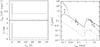Fig. 1 Refreshed shocks: forward shock model. Left panel: initial distribution of the Lorentz factor (lower part) and kinetic power (upper part) in the flow as a function of injection time tinj. Right panel: synthetic light curves at 2 eV (black, dotted line) and 10 keV (gray, dotted line) compared to the data from Perley et al. (2009). The kinetic energies injected in the spike and extended emission components are ${\mathit{E}}_{\mathrm{kin}}^{\mathrm{spike}}\mathrm{=}\mathrm{7}\mathrm{\times }{\mathrm{10}}^{\mathrm{50}}$ erg and ${\mathit{E}}_{\mathrm{kin}}^{\mathrm{ee}}\mathrm{=}\mathrm{50}{\mathit{E}}_{\mathrm{kin}}^{\mathrm{spike}}$. We adopt ${\mathit{ϵ}}_{\mathit{e}}\mathrm{=}{\mathit{ϵ}}_{\mathit{B}}^{\mathrm{1}\mathit{/}\mathrm{2}}\mathrm{=}\mathrm{5}\mathrm{\times }{\mathrm{10}}^{-2}$, p = 2.5 in the shocked external medium together with n = 10-3 cm-1 and z = 0.5. The steeper thin lines at late times correspond to a conical jet (seen on-axis) of opening angle θjet = 0.06 rad.

5.2.1. Forward shock model

In the standard forward shock model the lack of any detectable afterglow component before one day imposes severe constraints on either the density of the external medium or the values of the microphysics parameters. Fixing ϵ_e and ϵ_B to the commonly used values 0.1 and 0.01 implies to take n ≲ 10^-6 cm^-3 (Perley et al. 2009). This very low density would likely correspond to the intergalactic medium, which might be consistent with the absence of a candidate host galaxy down to a visual magnitude of 28.5. We preferred to adopt a less extreme value n = 10^-3 cm^-3, more typical of the interstellar medium at the outskirts of a galaxy (see e.g. Steidel et al. 2010). Then, decreasing the microphysics parameters to ${\mathit{ϵ}}_{\mathit{e}}\mathrm{=}{\mathit{ϵ}}_{\mathit{B}}^{\mathrm{1}\mathit{/}\mathrm{2}}\mathrm{=}\mathrm{0.05}$ becomes necessary to remain consistent with the data.

To obtain a rebrightning at one day we adopted Γ_ee = 20 and Γ_spike = 300. The outflow lasts for a total duration of 100 s (1 s for the the spike and 99 s for the tail). We injected a kinetic energy E_kin = 7 × 10⁵⁰ erg in the spike and 50 times more in the tail. It can be seen that the results, shown in Fig. 1, are consistent with the available data and upper limits except possibly after the peak of the rebrightening where the decline of the synthetic light curve is not steep enough. This can be corrected if a jet break occurs close to the peak, which is possible if the jet opening angle θ_jet is on the order of 1/Γ_ee ≃ 0.05 rad. This beaming angle is somewhat smaller than the values usually inferred from observations of short burst afterglows (see e.g. Burrows et al. 2006; Grupe et al. 2006) or suggested by simulations of compact binary mergers (see e.g. Rosswog & Ramirez-Ruiz 2002).

An example of a light curve with a jet break is shown in Fig. 1, assuming that the jet has an opening angle of 3.4° (0.06 rad) and is seen on-axis. A detailed study of the jet-break properties is beyond the scope of this paper and we therefore did not consider the case of an off-axis observer and neglected the lateral spreading of the jet, expected to become important when Γ ≲ 1/θ_jet. Detailed hydrodynamical studies (see e.g. Granot 2007; Zhang & MacFadyen 2009; van Eerten & MacFadyen 2011; Lyutikov 2012) tend to show, however, that as long as the outflow remains relativistic, the jet-break is more caused by the “missing” sideways emitting material than by jet angular spreading.

We finally checked how our results are affected if different model parameters are adopted. If the density n of the external medium is increased or decreased, similar light curves can be obtained by changing the Lorentz factors (to still achieve the rebrightning at one day) and the microphysics parameters (to recover the observed flux). For example, increasing the density to n = 0.1 cm^-3 requires Γ_ee ≃ 10 (keeping Γ_spike = 300) and ${\mathit{ϵ}}_{\mathit{e}}\mathrm{=}{\mathit{ϵ}}_{\mathit{B}}^{\mathrm{1}\mathit{/}\mathrm{2}}\mathrm{=}\mathrm{0.02}$. Conversely, with n = 10^-5 cm^-3, Γ_ee ≃ 35 and ${\mathit{ϵ}}_{\mathit{e}}\mathrm{=}{\mathit{ϵ}}_{\mathit{B}}^{\mathrm{1}\mathit{/}\mathrm{2}}\mathrm{=}\mathrm{0.08}$ are needed.

If the kinetic energy of the outflow is increased (resp. decreased) because the radiative efficiency f_rad is lower (resp. higher) or the redshift higher (resp. lower), light curves agreeing with the data can again be obtained by increasing (resp. decreasing) Γ_ee and decreasing (resp. increasing) ${\mathit{ϵ}}_{\mathit{e}}\mathrm{=}{\mathit{ϵ}}_{\mathit{B}}^{\mathrm{1}\mathit{/}\mathrm{2}}$. Also note that the spread of the Lorentz factor δΓ_ee around Γ_ee at the end of the prompt phase has to be limited to ensure that the slower material is able to catch up in a sufficiently short time to produce an effective rebrightening. In the case shown in Fig. 1 we have δΓ_ee/Γ_ee = 0 but we have checked from the numerical simulation that acceptable solutions can be obtained as long as δΓ_ee/Γ_ee ≲ 0.2. This configuration is for example naturally expected after an internal shock phase where fast and slow parts of the flow collide, resulting in a shocked region with a nearly uniform Lorentz factor distribution (see e.g. Daigne & Mochkovitch 2000).

5.2.2. Long-lived reverse shock model

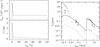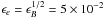
Fig. 2 Refreshed shocks: long-lived reverse shock model. Left panel: initial distribution of the Lorentz factor (lower part) and kinetic power (upper part) in the flow as a function of injection time tinj. Right panel: synthetic light-curves at 2 eV (black, dotted line) and 10 keV (grey, dotted line) together with the data. The kinetic energies in the spike and extended emission components are ${\mathit{E}}_{\mathrm{kin}}^{\mathrm{spike}}\mathrm{=}\mathrm{7}\mathrm{\times }{\mathrm{10}}^{\mathrm{50}}$ erg and ${\mathit{E}}_{\mathrm{kin}}^{\mathrm{ee}}\mathrm{=}\mathrm{30}{\mathit{E}}_{\mathrm{kin}}^{\mathrm{spike}}$. The density of the external medium, redshift and slope p of the electron distribution are the same as in Fig. 1. The adopted microphysics parameters are ${\mathit{ϵ}}_{\mathit{e}}\mathrm{=}{\mathit{ϵ}}_{\mathit{B}}^{\mathrm{1}\mathit{/}\mathrm{2}}\mathrm{=}\mathrm{0.16}$ in the shocked ejecta.

If the afterglow is produced by the reverse shock, similar good fits of the data can be obtained. Figure 2 shows an example of synthetic light curves for ${\mathit{E}}_{\mathrm{kin}}^{\mathrm{spike}}\mathrm{=}\mathrm{7}\mathrm{\times }{\mathrm{10}}^{\mathrm{50}}$ erg and ${\mathit{E}}_{\mathrm{kin}}^{\mathrm{ee}}\mathrm{=}\mathrm{30}{\mathit{E}}_{\mathrm{kin}}^{\mathrm{spike}}$, ${\mathit{ϵ}}_{\mathit{e}}\mathrm{=}{\mathit{ϵ}}_{\mathit{B}}^{\mathrm{1}\mathit{/}\mathrm{2}}\mathrm{=}\mathrm{0.16}$, p = 2.5 in the shocked ejecta and n = 10^-3 cm^-3. The microphysics parameters have to be higher than in the forward shock case because the reverse shock is dynamically less efficient, which requires a higher radiative efficiency to obtain the same observed fluxes. The Lorentz factor distribution in the ejecta is also slightly different to guarantee that the light curve (i) goes through the optical point at 0.05 day and (ii) decays steeply after the peak. No jet break has to be invoked here because the decay rate (in contrast to what happens in the forward shock model) depends on the distribution of energy as a function of the Lorentz factor in the ejecta.

Again, if the external density and kinetic energy of the flow are varied, satisfactory fits of the data can be recovered by slightly adjusting the Lorentz factor and microphysics parameters.

5.3. Density clump in the external medium

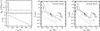Fig. 3 Density clump: forward and long-lived reverse shock models. Left panel: initial distribution of the Lorentz factor (lower part) and kinetic power (upper part) in the flow as a function of injection time tinj. Middle and right panels: synthetic light-curves at 2 eV (black) and 10 keV (grey) for the forward and reverse shocks, using either the simple one-zone (dotted lines) or the detailed multi-zone (dashed lines) model. The kinetic energies in the spike and extended emission components are ${\mathit{E}}_{\mathrm{kin}}^{\mathrm{spike}}\mathrm{=}\mathrm{7}\mathrm{\times }{\mathrm{10}}^{\mathrm{50}}$ erg and ${\mathit{E}}_{\mathrm{kin}}^{\mathrm{ee}}\mathrm{=}\mathrm{30}{\mathit{E}}_{\mathrm{kin}}^{\mathrm{spike}}$. The adopted microphysics parameters are ${\mathit{ϵ}}_{\mathit{e}}\mathrm{=}{\mathit{ϵ}}_{\mathit{B}}^{\mathrm{1}\mathit{/}\mathrm{2}}\mathrm{=}{\mathrm{10}}^{-2}$ (forward shock, middle panel) and ${\mathit{ϵ}}_{\mathit{e}}\mathrm{=}{\mathit{ϵ}}_{\mathit{B}}^{\mathrm{1}\mathit{/}\mathrm{2}}\mathrm{=}\mathrm{0.07}$ (reverse shock, right panel). See text for the prescription adopted for the density clump.

We now investigate the possibility that the rebrightening is caused by the encounter of the decelerating ejecta with a density clump in the external medium. For illustration, we adopted a simple distribution of the Lorentz factor that linearly decreases with injection time from 300 to 2 so that, in the absence of the density clump, afterglow light curves from either the forward or reverse shocks would be smooth and regular (we have checked that the exact shape of the low Lorentz factor tail is not crucial in this scenario). To model the clump, we assumed that the circumburst medium is uniform (with n = 10^-3 cm^-3) up to 1.7 × 10¹⁸ cm (0.55 pc) and that the density then rises linearly to n = 1 cm^-3 over a distance of 10¹⁸ cm (0.32 pc). The ejecta is strongly decelerated after entering the high-density region and we find that the forward shock is still inside the clump at the end of the calculation (at t_obs = 8 days).

5.3.1. Forward shock model

As Nakar & Granot (2007) showed by coupling their hydrodynamical calculation to a detailed radiative code, a density clump in the external medium has little effect on the forward shock emission. Therefore a clump cannot produce the rebrightening in GRB 080503. In the simple case where the shocked medium is represented by a single zone, the effect of the clump is barely visible. With the detailed multi-zone model a stronger rebrightening is found, because the effects of the compression resulting from the deceleration of the flow are better described, but even in this case the calculated flux remains nearly one order of magnitude below the data.

Figure 3 illustrates these results and confirms that the forward shock emission does not strongly react to the density clump. Even if, from an hydrodynamical point of view, the forward shock is sensitive to the clump, the observed synchrotron emission is only moderately affected because the increase in upstream density is nearly counterbalanced by the decrease of Lorentz factor in the shocked material. Of course, spectral effects complicate the picture, but the essence of the result remains the same (see Nakar & Granot 2007 for details).

5.3.2. Possible evolution of the microphysics parameters

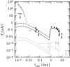Fig. 4 Density clump: forward shock model with varying microphysics parameters. Synthetic light-curves at 2 eV (black) and 10 keV (grey) when the microphysics parameters of the forward shock are changed at the density clump: ϵe is increased by a factor 5 from an initial value of 10-2, keeping the prescription ${\mathit{ϵ}}_{\mathit{e}}\mathrm{=}{\mathit{ϵ}}_{\mathit{B}}^{\mathrm{1}\mathit{/}\mathrm{2}}$. The Lorentz factor, injected kinetic power in the outflow, and the density distribution in the external medium are the same as in Fig. 3. The dotted and dashed lines correspond to the single and multi-zone models for the shocked region. The same simulations with the addition of a jet-break (assuming θjet = 0.08 rd) are also shown.

In view of the many uncertainties in the physics of collisionless shocks it is often assumed for simplicity, as we did so far, that the microphysics redistribution parameters ϵ_e and ϵ_B stay constant during the whole afterglow evolution. However, particle-in-cell simulations of acceleration in collisionless shocks (see e.g. Sironi & Spitkovsky 2011) do not show any evidence of universal values of the parameters. If ϵ_e or/and ϵ_B are allowed to change during afterglow evolution, the problem of the forward shock encountering a density clump can be reconsidered, now with the possibility of a sudden increase of radiative efficiency triggered by the jump in external density.

Figure 4 shows the resulting light curves when the microphysics parameters ϵ_e and ϵ_B of the forward shock are increased at the density clump. If the prescription ${\mathit{ϵ}}_{\mathit{e}}\mathrm{=}{\mathit{ϵ}}_{\mathit{B}}^{\mathrm{1}\mathit{/}\mathrm{2}}$ is maintained, no satisfactory solution can be found in the simple model where the shocked medium is represented by one single zone. In this case, the optical frequency lies between the injection and cooling frequencies (ν_i < ν_opt < ν_c) while the X-ray frequency satisfies ν_X > ν_c so that the visible and X-ray flux densities depend on the microphysics parameters in the following way (Panaitescu & Kumar 2000) 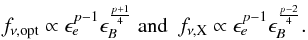${\mathit{f}}_{\mathit{\nu ,}\mathrm{opt}}\mathrm{\propto }{\mathit{ϵ}}_{\mathit{e}}^{\mathit{p}\mathrm{-}\mathrm{1}}{\mathit{ϵ}}_{\mathit{B}}^{\frac{\mathit{p}\mathrm{+}\mathrm{1}}{\mathrm{4}}}\mathrm{and}{\mathit{f}}_{\mathit{\nu ,}\mathrm{X}}\mathrm{\propto }{\mathit{ϵ}}_{\mathit{e}}^{\mathit{p}\mathrm{-}\mathrm{1}}{\mathit{ϵ}}_{\mathit{B}}^{\frac{\mathit{p}\mathrm{-}\mathrm{2}}{\mathrm{4}}}\mathit{.}$(3)With the prescription ${\mathit{ϵ}}_{\mathit{e}}\mathrm{=}{\mathit{ϵ}}_{\mathit{B}}^{\mathrm{1}\mathit{/}\mathrm{2}}$ we obtain ${\mathit{f}}_{\mathit{\nu ,}\mathrm{opt}}\mathrm{\propto }{\mathit{ϵ}}_{\mathit{e}}^{\frac{\mathrm{3}\mathit{p}\mathrm{-}\mathrm{1}}{\mathrm{2}}}$ and ${\mathit{f}}_{\mathit{\nu ,}\mathrm{X}}\mathrm{\propto }{\mathit{ϵ}}_{\mathit{e}}^{\frac{\mathrm{3}\mathit{p}\mathrm{-}\mathrm{4}}{\mathrm{2}}}$. The optical flux is therefore much more sensitive than the X-ray flux to a change of the microphysics parameters and a simultaneous fit of the data in both energy bands is not possible. A simple solution to this problem is to change ϵ_e alone, keeping ϵ_B constant. In this case, increasing ϵ_e by a factor of 25 (from 0.01 to 0.25) is required to reproduce the rebrightening in both the X-ray and visible ranges.

In the more detailed model with a multi-zone shocked region, the situation is different. In the shells that contribute most to the emission, we find that both ν_opt and ν_X are larger than ν_c and therefore f_ν,opt and f_ν,X depend in the same way on the microphysics parameters. It is then possible to achieve a satisfactory solution (dashed lines in Fig. 4) that keeps the prescription ${\mathit{ϵ}}_{\mathit{e}}\mathrm{=}{\mathit{ϵ}}_{\mathit{B}}^{\mathrm{1}\mathit{/}\mathrm{2}}$ (with ϵ_e increased by a factor 5). As in Sect. 5.2.1 we introduce a jet break (now assuming θ_jet = 0.08 rd) to account for the decay of the optical flux following the peak of the rebrightening. Notice that the decay is steeper here (compare Figs. 1 and 4) owing to the rapid decrease of the Lorentz factor inside the clump.

5.3.3. Long-lived reverse shock model

With the simple one-zone model, the reverse shock emission is found to be much more sensitive to the density clump than the forward shock emission. Indeed, when the ejecta starts to be decelerated, its bulk Lorentz factor suddenly decreases and slow shells from the tail material pile up at a high temporal rate and with a strong contrast in Lorentz factor. These two combined effects lead to a sharp rise of the flux from the reverse shock. Synthetic light curves showing a satisfactory agreement with the data are shown in Fig. 3.

However, the detailed multi-zone model gives different results, where the rebrightening is dimmer and cannot fit the data. The main reason is that the higher contrast in Lorentz factor, leading to a higher specific dissipated energy, now only concerns the freshly shocked shells, while in the single zone model it is applied to the whole shocked region. This example (as well as the one already discussed in Sect. 5.3.2) shows that using a detailed description of the shocked material can be crucial when dealing with complex scenarios (i.e. not the standard picture where the blast-wave propagates in a smooth external medium, with constant microphysics parameters)¹.

It is still possible to fit the data by increasing the microphysics parameters during the propagation in the clump. However, this seems less natural than for the forward shock (Sect. 5.3.2) because the upstream density of the reverse shock does not change. On the other hand, a modification of the microphysics parameters could still be due to the sudden increase in the reverse shock Lorentz factor triggered by the clump encounter.

6. Conclusion

GRB 080503 belongs to the special group of short bursts where an initial bright spike is followed by an extended soft emission of much longer duration. It did not show a transition to a standard afterglow after the steep decay observed in X-rays at the end of the extended emission. This behavior has been observed previously in short bursts, but GRB 080503 was peculiar because it exhibited a spectacular rebrightening after one day, both in X-rays and the visible. The presence of the extended emission prevents one from classifying GRB 080503 on the basis of duration only, but the lack of any candidate host galaxy at the location of the burst and the vanishing spectral lag of the spike component are consistent with its identification as a type-I event resulting from the coalescence of a binary system consisting of two compact objects.

From its formation to the coalescence, the system can migrate to the external regions of the host galaxy allowing the burst to occur in a very low density environment, accounting for the initial lack of a detectable afterglow. To explain the late rebrightening, we considered two possible scenarios – refreshed shocks from a late supply of energy or a density clump in the circumburst medium – and two models for the origin of the afterglow, the standard one where it comes from the forward shock and the alternative one where it is made by a long-lived reverse shock.

In the refreshed-shock scenario we supposed that the initial spike was produced by fast moving material (we adopted Γ = 300) while the one making the soft tail was slower (Γ ~ 20). Initially, only the spike material is decelerated and contributes to the afterglow until the tail material is eventually able to catch up, which produces the rebrightening. Both the forward and reverse shock models provide satisfactory fits of the data under the condition that the material making the tail has a limited spread in Lorentz factor δΓ/Γ ≲ 0.2. This allows the rise time of the rebrightening to be sufficiently short. This condition might be satisfied from the beginning but can also result from a previous sequence of internal shocks that has smoothed most of the fluctuations of the Lorentz factor initially present in the flow. In addition, a jet break is required in the forward shock case to reproduce the steep decline that follows the rebrightening. This implies that the jet should be beamed within an opening angle of 3–5°, which appears somewhat smaller than the values usually preferred for type-I bursts. In the long-lived reverse shock model a jet break is not necessary because the shape of the light curve now depends on the energy distribution in the ejecta, which can be adjusted to fit the data.

In the scenario where a density clump is present in the burst environment, the rebrightening resulting from the forward shock is weak, in agreement with the previous work of Nakar & Granot (2007). We performed the calculation in two ways: first with a simple method where the shocked material was represented by one single zone, then using a more detailed, multi-zone approach. The impact of the clump was barely visible in the first case. The rebrightening was larger in the second one but still remained nearly one order of magnitude below the data. We then considered the possibility that the shock microphysics might change inside the clump. We found that by increasing ϵ_e by a factor of five (and with the prescription that ${\mathit{ϵ}}_{\mathit{e}}\mathrm{=}{\mathit{ϵ}}_{\mathit{B}}^{\mathrm{1}\mathit{/}\mathrm{2}}$) it was possible to fit the data with the multi-zone model under the additional condition to have a jet break at about 2–3 days (corresponding to a jet opening angle  ≲ 5°). With the simplified model the results were more extreme, imposing to increase ϵ_e alone by a very large factor of 25.

If the afterglow is made by the reverse shock, the effect of the clump is strong with the simple model. It is however much reduced with the detailed model and the observed rebrightening cannot be reproduced, the synthetic light curve lying nearly one order of magnitude below the observed one. It appears that only the multi-zone approach provides a proper description of the compression resulting from the encounter with the density barrier. Conversely, in the refreshed-shock scenario the simple and detailed models give comparable results.

From the different possibilities we considered, which could explain the late rebrightening in GRB 080503, several appear compatible with the data, but none is clearly favored. The refreshed-shock scenario may seem more natural because the initial spike and extended emission probably correspond to different phases of central engine activity. It is not unreasonable to suppose that the material responsible for the extended emission had a lower Lorentz factor, as required by the refreshed-shock scenario. Then, both the forward and reverse shock models lead to satisfactory fits of the X-ray and visible light curves, if two

conditions on the Lorentz factor distribution and jet opening angle (see above) are satisfied. The density clump scenario does not seem able to account for the rebrightening if the afterglow is made by the reverse shock. The conclusion is the same with the forward shock, except if the microphysics parameters are allowed to change when the shock enters the clump.

Acknowledgments

The authors acknowledge the French Space Agency (CNES) for financial support. R.H.’s Ph.D. work is funded by a Fondation CFM-JP Aguilar grant.

References

All Figures

Fig. 1 Refreshed shocks: forward shock model. Left panel: initial distribution of the Lorentz factor (lower part) and kinetic power (upper part) in the flow as a function of injection time tinj. Right panel: synthetic light curves at 2 eV (black, dotted line) and 10 keV (gray, dotted line) compared to the data from Perley et al. (2009). The kinetic energies injected in the spike and extended emission components are ${\mathit{E}}_{\mathrm{kin}}^{\mathrm{spike}}\mathrm{=}\mathrm{7}\mathrm{\times }{\mathrm{10}}^{\mathrm{50}}$ erg and ${\mathit{E}}_{\mathrm{kin}}^{\mathrm{ee}}\mathrm{=}\mathrm{50}{\mathit{E}}_{\mathrm{kin}}^{\mathrm{spike}}$. We adopt ${\mathit{ϵ}}_{\mathit{e}}\mathrm{=}{\mathit{ϵ}}_{\mathit{B}}^{\mathrm{1}\mathit{/}\mathrm{2}}\mathrm{=}\mathrm{5}\mathrm{\times }{\mathrm{10}}^{-2}$, p = 2.5 in the shocked external medium together with n = 10-3 cm-1 and z = 0.5. The steeper thin lines at late times correspond to a conical jet (seen on-axis) of opening angle θjet = 0.06 rad.

In the text

Fig. 2 Refreshed shocks: long-lived reverse shock model. Left panel: initial distribution of the Lorentz factor (lower part) and kinetic power (upper part) in the flow as a function of injection time tinj. Right panel: synthetic light-curves at 2 eV (black, dotted line) and 10 keV (grey, dotted line) together with the data. The kinetic energies in the spike and extended emission components are ${\mathit{E}}_{\mathrm{kin}}^{\mathrm{spike}}\mathrm{=}\mathrm{7}\mathrm{\times }{\mathrm{10}}^{\mathrm{50}}$ erg and ${\mathit{E}}_{\mathrm{kin}}^{\mathrm{ee}}\mathrm{=}\mathrm{30}{\mathit{E}}_{\mathrm{kin}}^{\mathrm{spike}}$. The density of the external medium, redshift and slope p of the electron distribution are the same as in Fig. 1. The adopted microphysics parameters are ${\mathit{ϵ}}_{\mathit{e}}\mathrm{=}{\mathit{ϵ}}_{\mathit{B}}^{\mathrm{1}\mathit{/}\mathrm{2}}\mathrm{=}\mathrm{0.16}$ in the shocked ejecta.

In the text

Fig. 3 Density clump: forward and long-lived reverse shock models. Left panel: initial distribution of the Lorentz factor (lower part) and kinetic power (upper part) in the flow as a function of injection time tinj. Middle and right panels: synthetic light-curves at 2 eV (black) and 10 keV (grey) for the forward and reverse shocks, using either the simple one-zone (dotted lines) or the detailed multi-zone (dashed lines) model. The kinetic energies in the spike and extended emission components are ${\mathit{E}}_{\mathrm{kin}}^{\mathrm{spike}}\mathrm{=}\mathrm{7}\mathrm{\times }{\mathrm{10}}^{\mathrm{50}}$ erg and ${\mathit{E}}_{\mathrm{kin}}^{\mathrm{ee}}\mathrm{=}\mathrm{30}{\mathit{E}}_{\mathrm{kin}}^{\mathrm{spike}}$. The adopted microphysics parameters are ${\mathit{ϵ}}_{\mathit{e}}\mathrm{=}{\mathit{ϵ}}_{\mathit{B}}^{\mathrm{1}\mathit{/}\mathrm{2}}\mathrm{=}{\mathrm{10}}^{-2}$ (forward shock, middle panel) and ${\mathit{ϵ}}_{\mathit{e}}\mathrm{=}{\mathit{ϵ}}_{\mathit{B}}^{\mathrm{1}\mathit{/}\mathrm{2}}\mathrm{=}\mathrm{0.07}$ (reverse shock, right panel). See text for the prescription adopted for the density clump.

In the text

Fig. 4 Density clump: forward shock model with varying microphysics parameters. Synthetic light-curves at 2 eV (black) and 10 keV (grey) when the microphysics parameters of the forward shock are changed at the density clump: ϵe is increased by a factor 5 from an initial value of 10-2, keeping the prescription ${\mathit{ϵ}}_{\mathit{e}}\mathrm{=}{\mathit{ϵ}}_{\mathit{B}}^{\mathrm{1}\mathit{/}\mathrm{2}}$. The Lorentz factor, injected kinetic power in the outflow, and the density distribution in the external medium are the same as in Fig. 3. The dotted and dashed lines correspond to the single and multi-zone models for the shocked region. The same simulations with the addition of a jet-break (assuming θjet = 0.08 rd) are also shown.

In the text

References

- Barkov, M. V., & Pozanenko, A. S. 2011, MNRAS, 417, 2161 [NASA ADS] [CrossRef] [Google Scholar]
- Barthelmy, S. D., Chincarini, G., Burrows, D. N., et al. 2005, Nature, 438, 994 [NASA ADS] [CrossRef] [PubMed] [Google Scholar]
- Belczynski, K., Perna, R., Bulik, T., et al. 2006, ApJ, 648, 1110 [NASA ADS] [CrossRef] [Google Scholar]
- Beloborodov, A. M. 2005, ApJ, 627, 346 [NASA ADS] [CrossRef] [Google Scholar]
- Beloborodov, A. M. 2010, MNRAS, 407, 1033 [NASA ADS] [CrossRef] [Google Scholar]
- Berger, E. 2009, ApJ, 690, 231 [NASA ADS] [CrossRef] [Google Scholar]
- Berger, E., Price, P. A., Cenko, S. B., et al. 2005, Nature, 438, 988 [NASA ADS] [CrossRef] [PubMed] [Google Scholar]
- Bloom, J. S., & Prochaska, J. X. 2006, in Gamma-Ray Bursts in the Swift Era, ed. S. S. Holt, N. Gehrels, & J. A. Nousek, AIP Conf. Ser., 836, 473 [Google Scholar]
- Burrows, D. N., Grupe, D., Capalbi, M., et al. 2006, ApJ, 653, 468 [NASA ADS] [CrossRef] [Google Scholar]
- Daigne, F., & Mochkovitch, R. 1998, MNRAS, 296, 275 [Google Scholar]
- Daigne, F., & Mochkovitch, R. 2000, A&A, 358, 1157 [NASA ADS] [Google Scholar]
- Drenkhahn, G., & Spruit, H. C. 2002, A&A, 391, 1141 [NASA ADS] [CrossRef] [EDP Sciences] [Google Scholar]
- Fox, D. B., Frail, D. A., Price, P. A., et al. 2005, Nature, 437, 845 [NASA ADS] [CrossRef] [PubMed] [Google Scholar]
- Gehrels, N., Sarazin, C. L., O’Brien, P. T., et al. 2005, Nature, 437, 851 [NASA ADS] [CrossRef] [PubMed] [Google Scholar]
- Gehrels, N., Norris, J. P., Barthelmy, S. D., et al. 2006, Nature, 444, 1044 [NASA ADS] [CrossRef] [PubMed] [Google Scholar]
- Genet, F., Daigne, F., & Mochkovitch, R. 2007, MNRAS, 381, 732 [NASA ADS] [CrossRef] [Google Scholar]
- Giannios, D., & Spruit, H. C. 2006, A&A, 450, 887 [NASA ADS] [CrossRef] [EDP Sciences] [Google Scholar]
- Granot, J. 2005, ApJ, 631, 1022 [NASA ADS] [CrossRef] [Google Scholar]
- Granot, J. 2007, Rev. Mex. Astron. Astrofis. Conf. Ser., 27, 140 [NASA ADS] [Google Scholar]
- Granot, J., Panaitescu, A., Kumar, P., & Woosley, S. E. 2002, ApJ, 570, L61 [NASA ADS] [CrossRef] [Google Scholar]
- Grupe, D., Burrows, D. N., Patel, S. K., et al. 2006, ApJ, 653, 462 [NASA ADS] [CrossRef] [Google Scholar]
- Hjorth, J., Watson, D., Fynbo, J. P. U., et al. 2005, Nature, 437, 859 [NASA ADS] [CrossRef] [PubMed] [Google Scholar]
- Hobbs, G., Lorimer, D. R., Lyne, A. G., & Kramer, M. 2005, MNRAS, 360, 974 [NASA ADS] [CrossRef] [Google Scholar]
- Kouveliotou, C., Meegan, C. A., Fishman, G. J., et al. 1993, ApJ, 413, L101 [NASA ADS] [CrossRef] [Google Scholar]
- Li, L.-X., & Paczyński, B. 1998, ApJ, 507, L59 [Google Scholar]
- Lyutikov, M. 2012, MNRAS, 421, 522 [NASA ADS] [Google Scholar]
- Mao, J., Guidorzi, C., Ukwatta, T., et al. 2008, GCN Report, 138, 1 [NASA ADS] [Google Scholar]
- McKinney, J. C., & Uzdensky, D. A. 2012, MNRAS, 419, 573 [Google Scholar]
- Medvedev, M. V. 2006, ApJ, 651, L9 [NASA ADS] [CrossRef] [Google Scholar]
- Meszaros, P., & Rees, M. J. 1997, ApJ, 476, 232 [NASA ADS] [CrossRef] [Google Scholar]
- Metzger, B. D., Quataert, E., & Thompson, T. A. 2008, MNRAS, 385, 1455 [NASA ADS] [CrossRef] [Google Scholar]
- Mochkovitch, R., Hernanz, M., Isern, J., & Martin, X. 1993, Nature, 361, 236 [NASA ADS] [CrossRef] [Google Scholar]
- Nakar, E. 2007, Phys. Rep., 442, 166 [NASA ADS] [CrossRef] [Google Scholar]
- Nakar, E., & Granot, J. 2007, MNRAS, 380, 1744 [NASA ADS] [CrossRef] [Google Scholar]
- Narayan, R., Paczynski, B., & Piran, T. 1992, ApJ, 395, L83 [NASA ADS] [CrossRef] [Google Scholar]
- Norris, J. P., & Bonnell, J. T. 2006, ApJ, 643, 266 [NASA ADS] [CrossRef] [Google Scholar]
- Panaitescu, A., & Kumar, P. 2000, ApJ, 543, 66 [NASA ADS] [CrossRef] [Google Scholar]
- Perley, D. A., Metzger, B. D., Granot, J., et al. 2009, ApJ, 696, 1871 [NASA ADS] [CrossRef] [Google Scholar]
- Rees, M. J., & Meszaros, P. 1994, ApJ, 430, L93 [NASA ADS] [CrossRef] [Google Scholar]
- Rees, M. J., & Meszaros, P. 1998, ApJ, 496, L1 [NASA ADS] [CrossRef] [Google Scholar]
- Rees, M. J., & Mészáros, P. 2005, ApJ, 628, 847 [NASA ADS] [CrossRef] [Google Scholar]
- Rosswog, S. 2007, MNRAS, 376, L48 [NASA ADS] [Google Scholar]
- Rosswog, S., & Ramirez-Ruiz, E. 2002, MNRAS, 336, L7 [NASA ADS] [CrossRef] [Google Scholar]
- Ruffert, M., & Janka, H.-T. 1999, A&A, 344, 573 [NASA ADS] [Google Scholar]
- Sakamoto, T., & Gehrels, N. 2009, in AIP Conf. Ser. 1133, ed. C. Meegan, C. Kouveliotou, & N. Gehrels, 112 [Google Scholar]
- Sari, R., & Mészáros, P. 2000, ApJ, 535, L33 [NASA ADS] [CrossRef] [PubMed] [Google Scholar]
- Sari, R., Piran, T., & Narayan, R. 1998, ApJ, 497, L17 [NASA ADS] [CrossRef] [Google Scholar]
- Sironi, L., & Spitkovsky, A. 2011, ApJ, 726, 75 [NASA ADS] [CrossRef] [Google Scholar]
- Soderberg, A. M., Berger, E., Kasliwal, M., et al. 2006, ApJ, 650, 261 [NASA ADS] [CrossRef] [Google Scholar]
- Spruit, H. C., Daigne, F., & Drenkhahn, G. 2001, A&A, 369, 694 [NASA ADS] [CrossRef] [EDP Sciences] [Google Scholar]
- Steidel, C. C., Erb, D. K., Shapley, A. E., et al. 2010, ApJ, 717, 289 [NASA ADS] [CrossRef] [Google Scholar]
- Troja, E., King, A. R., O’Brien, P. T., Lyons, N., & Cusumano, G. 2008, MNRAS, 385, L10 [NASA ADS] [CrossRef] [Google Scholar]
- Uhm, Z. L., & Beloborodov, A. M. 2007, ApJ, 665, L93 [NASA ADS] [CrossRef] [Google Scholar]
- van Eerten, H. J., & MacFadyen, A. I. 2011 [arXiv:1105.2485] [Google Scholar]
- Villasenor, J. S., Lamb, D. Q., Ricker, G. R., et al. 2005, Nature, 437, 855 [NASA ADS] [CrossRef] [PubMed] [Google Scholar]
- Zhang, B. 2006, Nature, 444, 1010 [NASA ADS] [CrossRef] [Google Scholar]
- Zhang, W., & MacFadyen, A. 2009, ApJ, 698, 1261 [NASA ADS] [CrossRef] [Google Scholar]