© ESO, 2012

1. Introduction

Sensitivity and resolution (both spectral and angular) are the main limiting factors in observational astronomy. In the case of angular (i.e., spatial) resolution, the strong limitation of all observations, regardless of the quality of our instruments, is the diffraction limit. When an instrument is diffraction-limited, its response to a plane wave (i.e., to a point source located at infinity) is the so-called point spread function (PSF), which has a width related to the smallest angular scale that can be resolved with the instrument.

It is well-known that the diffraction limit decreases with both an increasing observing frequency and an increasing aperture of the instrument. Hence, the only way to achieve a higher angular resolution at a given frequency is to increase the instrument aperture. In this sense, the aperture synthesis, which is a technique related to astronomical interferometry (see, e.g., Thomson et al. 1986), presently seems to be almost the only way to further increase the angular resolution currently achieved at any wavelength.

However, interferometric observations differ in a crucial way from those obtained with other techniques. When aperture synthesis is performed, an interferometer does not directly observe the structure of a source, but samples fractions of its Fourier transform (the so-called visibilities). In other words, the space from which an interferometer takes measurements is not the sky itself, but the Fourier transform of its intensity distribution over the whole field of view. This special characteristic of interferometers strongly affects how these devices behave when we observe sources of sizes well below the diffraction limit, as we illustrate in the following sections.

It is possible, of course, to compute the inverse Fourier transform of a set of visibilities and (try to) recover the intensity distribution of the observed sources in the sky. When combined with certain deconvolution algorithms, this approach of imaging a set of visibilities may be very useful when dealing with relatively extended sources. However, if the sources observed are very compact (relative to the diffraction limit of the interferometer), important and uncontrollable effects may arise in the imaging of the source intensity profiles, either from the (non-linear) deconvolution algorithms and/or from the gridding (pixelation) in the sky plane. These effects may result in strong biases in the estimate of source sizes, based on measurements performed in the sky plane.

The over-resolution power of an interferometer is a function of the baseline sensitivity, and may play an important role in the analysis of data coming from future ultra-sensitive interferometric arrays (such as the Square Kilometer Array, SKA, or the Atacama Large Millimeter/sub-millimeter Array, ALMA).

In this research note, we review several well-known effects of source compactness in visibility space, showing that it is possible to find out, from the observed visibilities, information on the size of sources that are much smaller than the diffraction limit achieved in the aperture synthesis. We also estimate the maximum theoretical over-resolution power of an interferometer and discuss a statistical test to estimate upper bounds to the size of ultra-compact sources observed with high-sensitivity interferometers.

2. Compact sources in visibility space

The size of a source slightly smaller than the diffraction limit of an interferometer leaves a very clear fingerprint in visibility space, although its effect on the sky plane (after all the imaging and deconvolution steps) may be much less clear. For instance, if the size of a source is similar to the full width at half maximum (FWHM) of the PSF, the radial profile in the visibility amplitudes will decrease with baseline length falling down to  ~ 0.5 times the maximum visibility amplitude at the maximum projected baseline. Hence, a source with a size of the order of the diffraction limit maps into an amplitude profile in visibility space that can be well-detected and characterized by an interferometer.

When the size of the source decreases, the visibility amplitude in the longest baseline increases; in the limiting case when the size of the source tends to zero, the visibility amplitude in the longest baseline tends to be as large as that in the shortest baseline. It is common, indeed, to compute the amplitude ratio of the visibilities in the shortest baseline to those in the longest baseline as a quantitative representation of the degree of compactness of the observed sources (e.g., Kovalev et al. 2005).

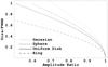Fig. 1 Source size (in units of the FWHM of the synthesized beam) as a function of the ratio of the visibility amplitude in the longest baseline to that in the shortest baseline.

In Fig. 1, we show the size of a source as a function of the visibility amplitude in the longest baseline divided by that in the shortest baseline. The size shown in Fig. 1 is given in units of the FWHM of the synthesized beam (we assume throughout this paper that uniform weighting is applied to the gridding of the visibilities, prior to the Fourier inversion; see Thomson et al. 1986, for more details). If the sensitivity of an interferometer allows us to detect a small decrease in the visibility amplitudes at the longest baselines, we are able to obtain information on the size of sources much smaller than the diffraction limit of the interferometer (i.e., much smaller than the FWHM of the PSF). The over-resolution power of an interferometer, hence, depends on the sensitivity of the observations, and can be arbitrarily large.

Figure 1 has been computed using a different intensity profiles for the observed source. It is obvious that the use of different source shapes (e.g., a Gaussian profile or a ring-like source) in a fit to the visibilities, results in different size estimates for the same dataset. Hence, if the structure of the observed source is similar to the model used in the fit to the visibilities (i.e., if we have reliable a priori information on the real shape of the source), we can obtain precise estimates of sizes that are much smaller than the FWHM of the synthesized beam.

The extrapolation power of model fitting over the diffraction limit has been well known for a long time, because in these cases the data are fitted with a simple model (i.e., with a small number of parameters), in contrast to the image-synthesis approach, where the super-resolution capabilities are far more limited owing to the larger parameter space of the model (i.e., the image pixels). Therefore, it is very difficult to obtain, from any data analysis based on the sky plane, size estimates of compact sources with a precision similar to that achieved in Fourier space. In the former case, the gridding of the images (i.e., the pixelation of the PSF), together with the particulars of the deconvolution algorithms, may smear out the fine details in the intensity profiles that encode the information on the structures of the underlying compact sources. On the other hand, compact sources on the sky are seen as very extended structures in Fourier space. Thus, a direct analysis of the visibilities (e.g., as described in Pearson 1999) is the optimal way to analyze data coming from compact sources, since the effects of gridding in Fourier space will always be negligible.

3. Maximum theoretical over-resolution power of an interferometer

As described in the previous section, the maximum over-resolution power of an interferometer (i.e., the minimum size of a source, in units of the FWHM of the synthesized beam, that can be resolved) depends on how precisely we can measure lower visibility amplitudes at the longest baselines. Hence, an interferometer with an arbitrarily high sensitivity will accordingly have an arbitrarily high over-resolution power.

However, real interferometers have finite sensitivities that depend on several factors (e.g., observing frequency, bandwidth, source coordinates, weather conditions, ...). We can therefore ask what is the minimum size of a source (relative to the diffraction limit of an interferometer) that still allows us to extract size information from the observed visibilities.

In the extreme case of a very compact (and/or weak) source, such that it impossible to estimate a statistically significant lowering in the visibility amplitudes at the longest baselines (because of the noise contribution to the visibilities), the only meaningful statistical analysis that can be applied to the data is to estimate an upper limit to the source size by means of hypothesis testing.

We observe a source and assume the null hypothesis, H₀, that it has no structure at all (i.e., the source is point-like, so the visibility amplitudes are constant throughout Fourier space). The likelihood, Λ₀, corresponding to a point-like model source fitted to the visibilities is 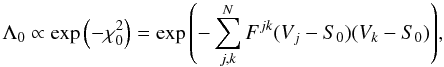${\mathrm{\Lambda }}_{\mathrm{0}}\mathrm{\propto }\exp \mathrm{(}\mathrm{-}{{\mathit{\chi }}_{\mathrm{0}}^{\mathrm{2}}}^{\mathrm{)}}\mathrm{=}\exp \left(\mathrm{-}\sum _{\mathit{j,k}}^{\mathit{N}}{\mathit{F}}^{\mathit{jk}}\mathrm{(}{\mathit{V}}_{\mathit{j}}\mathrm{-}{\mathit{S}}_{\mathrm{0}}\mathrm{)}\mathrm{(}{\mathit{V}}_{\mathit{k}}\mathrm{-}{\mathit{S}}_{\mathrm{0}}\mathrm{)}\right)\mathit{,}$(1)where N is the number of visibilities, V_j = A_jexp(iφ_j) is the jth visibility, S₀ is the maximum-likelihood (ML) estimate of the source flux density (it can be shown to be equal to the real part of the weighted visibility average,  ⟨ V ⟩ ), and F is the Fisher matrix of the visibilities (i.e., the inverse of the their covariance matrix), i.e.

$\mathit{F}\mathrm{=}{\mathit{C}}^{-1} \mathrm{with} {\mathit{C}}_{\mathit{j,k}}\mathrm{=}{\mathit{\rho }}_{\mathit{jk}}{\mathit{\sigma }}_{\mathit{j}}{\mathit{\sigma }}_{\mathit{k}}\mathit{.}$In this equation, ρ_jk is the correlation coefficient between the jth and kth visibility, and σ_j is the uncertainty in the jth visibility. Equation (1) is generic and accounts for any correlation in the visibilities (e.g., possible global or antenna-dependent amplitude biases). It can be shown that log Λ₀ follows a χ² distribution (close to its maximum) with a number of degrees of freedom equal to the rank of matrix F minus unity. In the particular case when there is no correlation between visibilities¹, the number of degrees of freedom equals N − 1.

We model the visibilities with a function, V^m(S,q   θ), which corresponds to the model of a (symmetric) source of size θ and flux density S (the model amplitude, V^m, depends on the product of θ times the distance in Fourier space, q). Hence, the visibility V_j is modelled by the amplitude ${\mathit{V}}_{\mathit{j}}^{\mathit{m}}\mathrm{=}{\mathit{V}}^{\mathit{m}}\mathrm{(}\mathit{S,}{\mathit{q}}_{\mathit{j}}\hspace{0.17em}\mathit{\theta }\mathrm{)}$. The likelihood of this new modelling, Λ_m, is also given by Eq. (1), but where S₀ is changed to V^m. In addition, the distribution of log Λ_m (close to its maximum value) also follows a χ² distribution, but with one degree of freedom less than that of log Λ₀.

We now consider the maximum value of θ (which we call θ_M) corresponding to a value of the log-likelihood of V^m that is compatible, by chance, with the parent distribution of the log-likelihood of a point source. We estimate θ_M by computing the critical probability for the hypothesis that both quantities come from the same parent distribution (this is, indeed, our null hypothesis, H₀). Critical probabilities of 5% and 0.3% are used in our hypothesis testing (these values correspond to the 2σ and 3σ cutoffs of a Gaussian distribution, respectively). The value of θ_M estimated in this way is the maximum size that the observed source may have, such that the interferometer could have measured the observed visibilities with a probability given by the critical probability of H₀.

The log-likelihood ratio (in our case, the difference in the chi-squares; see Mood et al. 1974) between the model of a point source and that of a source with visibilities modelled by V^m follows a χ² distribution with one degree of freedom, as long as N is large (e.g., Wilks 1938). Hence, H₀ is not discarded as long as $\log {\mathrm{\Lambda }}_{\mathit{m}}\mathrm{-}\log {\mathrm{\Lambda }}_{\mathrm{0}}\mathit{<}{\mathit{\lambda }}_{\mathrm{c}}\mathit{/}\mathrm{2}\mathit{,}$(2)where λ_c is the value of the log-likelihood corresponding to the critical probability of the null hypothesis for a χ² distribution with one degree of freedom. The values of λ_c are 3.84 or 8.81 (for a 5% and a 0.3% probability cuttoff of H₀, respectively). Working out Eq. (2), we arrive at 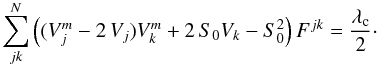$\sum _{\mathit{jk}}^{\mathit{N}}\mathrm{\left(}\mathrm{\right(}{\mathit{V}}_{\mathit{j}}^{\mathit{m}}\mathrm{-}\mathrm{2}\hspace{0.17em}{\mathit{V}}_{\mathit{j}}\mathrm{)}{\mathit{V}}_{\mathit{k}}^{\mathit{m}}\mathrm{+}\mathrm{2}\hspace{0.17em}{\mathit{S}}_{\mathrm{0}}{\mathit{V}}_{\mathit{k}}\mathrm{-}{{\mathit{S}}_{\mathrm{0}}^{\mathrm{2}}}^{\mathrm{)}}{\mathit{F}}^{\mathit{jk}}\mathrm{=}\frac{{\mathit{\lambda }}_{\mathrm{c}}}{\mathrm{2}}\mathrm{·}$(3)We can simplify Eq. (3) in the special case when the off-diagonal elements in the covariance matrix are small (thus the visibilities are nearly independent). 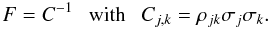The standard deviation, σ, of the weighted visibility average is 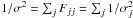$\mathrm{1}\mathit{/}{\mathit{\sigma }}^{\mathrm{2}}\mathrm{=}{\sum }_{\mathit{j}}{\mathit{F}}_{\mathit{jj}}\mathrm{=}{\sum }_{\mathit{j}}\mathrm{1}\mathit{/}{\mathit{\sigma }}_{\mathit{j}}^{\mathrm{2}}$, whereas the weighted average of any visibility-related quantity, A, is  ⟨ A ⟩  = σ² ∑ _jF_jjA_j. Hence, if F_jk ~ 0 for j ≠ k (i.e., if both matrices, F and C = F^-1 are diagonal), we have $\mathrm{⟨}{\left({\mathit{V}}^{\mathit{m}}\right)}^{\mathrm{2}}\mathrm{+}{\mathit{S}}_{\mathrm{0}}^{\mathrm{2}}\mathrm{-}\mathrm{2}\mathit{V}{\mathit{V}}^{\mathit{m}}\mathrm{⟩}\mathrm{~}\mathrm{⟨}{\left({\mathit{S}}_{\mathrm{0}}\mathrm{-}{\mathit{V}}^{\mathit{m}}\right)}^{\mathrm{2}}\mathrm{⟩}\mathrm{=}\frac{{\mathit{\lambda }}_{\mathrm{c}}{\mathit{\sigma }}^{\mathrm{2}}}{\mathrm{2}}\mathit{,}$(4)i.e., the critical probability in our hypothesis testing depends on the weighted average of the quadratic difference between the two models being compared (a point source with flux density S₀ =  ⟨ V ⟩  and an extended source with a model given by V^m). In this equation, it is assumed that  ⟨ VV^m ⟩  ~  ⟨ S₀V^m ⟩ . Indeed

$\mathrm{⟨}\mathit{V}{\mathit{V}}^{\mathit{m}}\mathrm{⟩}\mathrm{=}\mathrm{⟨}{\mathit{S}}_{\mathrm{0}}{\mathit{V}}^{\mathit{m}}\mathrm{⟩}\mathrm{+}\mathrm{⟨}\mathrm{(}\mathit{V}\mathrm{-}{\mathit{S}}_{\mathrm{0}}\mathrm{)}{\mathit{V}}^{\mathit{m}}\mathrm{⟩}\mathit{.}$Since the source is compact in terms of the diffraction limit of the interferometer (otherwise, this hypothesis testing would not be meaningful), the dependence of V^m on the distance in Fourier space, q, will be small (i.e., the best-fitting model V^m will be almost constant for the whole set of observations). As long as the decrease in V^m with q is smaller than the standard deviation in the visibilities (which holds if there is no hint of a decrease in the visibility amplitudes with q), the quantity  ⟨ (V − S₀)V^m ⟩  will always approach zero (we note that  ⟨ (V − S₀) ⟩  = 0). Hence, from Eq. (4), we can finally write that

$⟨{\left(\mathrm{1}\mathrm{-}\frac{{\mathit{V}}^{\mathit{m}}}{\mathrm{⟨}\mathit{V}\mathrm{⟩}}\right)}^{\mathrm{2}}⟩\mathrm{=}\frac{{\mathit{\lambda }}_{\mathrm{c}}}{\mathrm{2}\mathrm{(}\mathit{S}\mathit{/}\mathit{N}{\mathrm{)}}^{\mathrm{2}}}\mathit{,}$(5)

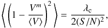
where S/N is the signal-to-noise ratio of the weighted visibility average (i.e.,  ⟨ V ⟩ /σ). If the covariance matrix is far from being diagonal, Eq. (5) does not apply, since the off-diagonal elements in Eq. (3) are then added to the left-hand side of Eq. (5)). However, it can be shown that if all the off-diagonal elements of F_jk are roughly equal and  ⟨ V ⟩  ~  ⟨ V^m ⟩  ~ S₀ (which is true if both models V^m and a point source S₀ satisfactorily fit the data), then the combined effect of the off-diagonal elements in Eq. (3) cancels out, and Eq. (5) still applies.

This restriction for the F matrix (hence the correlation matrix) can be interpreted in the following way. A distribution of visibilities following a covariance matrix with roughly equal off-diagonal elements implies that all the antennas in the interferometer should have similar sensitivities, and the baselines related to each one of them should cover the full range of distances in Fourier space. If these conditions are fulfilled, it is always possible to remove any bias in the antenna gains, and produce a set of visibilities with a roughly equal covariance between them. If, for instance, the gain at one antenna were biased, the visibilities of the baselines of all the other antennas would have different amplitudes in similar regions of the Fourier space, hence allowing us to correct for that bias by means of amplitude self-calibration. However, if the array were sparse, there might be antenna-related amplitude biases affecting visibilities at disjoint regions of Fourier space, thus preventing the correction for these biases using closeby measurements from baselines of other antennas. Interferometers with a sparse distribution of elements may thus produce sets of visibilities with different covariances (stronger at closer regions in Fourier space), thus making it difficult to estimate θ_M correctly (unless in the very unlikely cases when the whole matrix F is known!). This is the case of the NRAO Very Long Baseline Array (VLBA), where the antennas at Mauna Kea and St. Croix only appear on the longest baselines; lower visibility amplitudes at these baselines could thus be related to biased antenna gains, instead of source structure.

The new interferometric arrays, which consist of many similar elements with a smooth spatial distribution (such as ALMA or the SKA) almost fulfill the condition of homogeneous Fourier coverage described here (i.e., there are almost no antennas that exclusively appear at long or short baselines), and are hence very robust to the over-resolution of compact sources well below their diffraction limits.

Equation (5) allows us to estimate the value of θ_M from a given distribution of baseline lengths, q_j, and for a given S/N in the weighted visibility average. We now assume that we have a very large number of visibilities and that the sampling of baseline lengths, q_j, is quasi-continuous. We then have

${\mathrm{\int }}_{\mathrm{0}}^{\mathit{Q}}\mathit{n}\mathrm{\left(}\mathit{q}\mathrm{\right)}\hspace{0.17em}\mathrm{(}\mathrm{1}\mathrm{-}\frac{\mathrm{1}}{\mathrm{⟨}\mathit{V}\mathrm{⟩}}{\mathit{V}}_{\mathit{m}}\mathrm{(}\mathit{S,q}\hspace{0.17em}{\mathit{\theta }}_{\mathit{M}}\mathrm{)}{\mathrm{)}}^{\mathrm{2}}\hspace{0.17em}\mathrm{d}\mathit{q}\mathrm{=}\frac{{\mathit{\lambda }}_{\mathrm{c}}}{\mathrm{2}\mathrm{(}\mathit{S}\mathit{/}\mathit{N}{\mathrm{)}}^{\mathrm{2}}}\mathit{,}$(6)

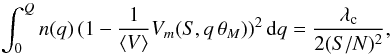
where n(q) is the (normalized) density of visibilities at a distance q in Fourier space and Q is the maximum baseline length of the interferometer. Usually, n(q) is large for small values of q and decreases with increasing q (i.e., the number of short baselines is usually larger than the number of long baselines)². The effect of n(q) on θ_M is such that an interferometer with a large number of long baselines has a higher over-resolution power than another interferometer with a lower number of long baselines, even if the maximum baseline length, Q, is the same for both interferometers. The over-resolution power can also be increased if we decrease the right-hand sides of Eqs. (5) and (6). This can be achieved by increasing the sensitivity of the antennas and/or the observing time, even if the maximum baseline length is unchanged.

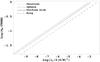Fig. 2 Minimum detectable size of a source (in units of the FWHM of the synthesized beam) as a function of the source model (for a constant density of baseline lengths).

We show in Fig. 2 the value of θ_M (in units of the FWHM of the synthesized beam) corresponding to different array sensitivities (i.e., different S/N in the visibility average) and source models (i.e., Gaussian, uniform-disk, sphere, and ring). We use a baseline-length distribution with a constant density (a constant n(q)). In all cases, the over-resolution power of the interferometer can be closely approximated by the expression

${\mathit{\theta }}_{\mathit{M}}\mathrm{=}\mathit{\beta }\hspace{0.17em}{\left(\frac{{\mathit{\lambda }}_{\mathrm{c}}}{\mathrm{2}\mathrm{(}\mathit{S}\mathit{/}\mathit{N}{\mathrm{)}}^{\mathrm{2}}}\right)}^{\mathrm{1}\mathit{/}\mathrm{4}}\mathrm{\times }\mathit{FWHM}\mathit{,}$(7)

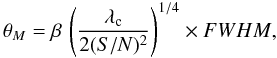
where β slightly depends on the shape of n(q) and the intensity profile of the source model. It usually takes values in the range 0.5–1.0 (it is larger for steeper n(q) and/or for source intensity profiles with higher intensities at smaller scales).

We note that in the more general case, θ_M should be solved directly from Eq. (5) (or even from Eq. (3), if the array was sparse and/or the covariance matrix was far from homogeneous or diagonal). We note that θ_M in Fig. 2 can be interpreted in two different ways, as either the maximum possible size of a source that generates visibilities compatible with a point-like source or the true minimum size of a source that can still be resolved by the interferometer. Any of these two (equivalent) interpretations of θ_M lead us to the conclusion that an interferometer is capable of resolving structures well below the mere diffraction limit achieved in the aperture synthesis.

In the cases of ultra-sensitive interferometric arrays such as the SKA, where dynamic ranges of even 10⁶ will be eventually

achieved in the images, the over-resolution power in observations of strong and compact sources can be very large. As an example, a dedicated observation with the SKA (which we assume to consist of 200 antennas) over one hour (with an integration time of 2 s), and an S/N of 100 for each visibility, results in a minimum resolvable size of only  ~2 × 10^-3 times the FWHM of the synthesized beam (Eq. (7)). As a result, and depending on the observing frequency, the over-resolution power of the SKA would allow us to study details of sources on angular scales as small as a few μas. This is, indeed, a higher resolution than the diffraction limit achieved with the current VLBI arrays (i.e., using much longer baselines).

4. Summary

We have reviewed the effects of source compactness in interferometric observations. The analysis of visibilities in Fourier space allows us to estimate the sizes of very compact sources (which are much smaller than the diffraction limit achieved in the aperture synthesis). As the sensitivity of the interferometer increases, the minimum size of the sources that can still be resolved decreases (i.e., the over-resolution power of the interferometer increases). In this sense, the analysis of observations of very compact sources in Fourier space is more reliable (and robust) than alternative analyses based on synthesized images of the sky intensity distribution (and affected by beam gridding, deconvolution biases, etc.).

We have studied the case of extremely compact sources observed with an interferometer of finite sensitivity. If the source is so compact and/or weak that it is impossible to detect structure in the visibilities, we describe a test of hypothesis to set a strong upper limit to the size of the source. We also compute the minimum possible size of a source whose structure can still be resolved by an interferometer (i.e., the maximum theoretical over-resolution power of an interferometer, computed from Eq. (5) and approximated in Eq. (7)). The over-resolution power depends on the number of visibilities, the array sensitivity, and the spatial distribution of the baselines, and increases if: 1) the number of long baselines increases (i.e., not necessarily the maximum baseline length, but only the number of long baselines relative to the number of short baselines); 2) the observing time lengthens; and/or 3) the array sensitivity increases.

Acknowledgments

The authors wish to thank J. M. Anderson for helpful discussion and the anonymous referee for his/her useful comments. M.A.P.T. acknowledges support through grant AYA2006-14986-C02-01 (MEC), and grants FQM-1747 and TIC-126 (CICE, Junta de Andalucía).

References

All Figures

	Fig. 1 Source size (in units of the FWHM of the synthesized beam) as a function of the ratio of the visibility amplitude in the longest baseline to that in the shortest baseline.
In the text

	Fig. 2 Minimum detectable size of a source (in units of the FWHM of the synthesized beam) as a function of the source model (for a constant density of baseline lengths).
In the text

References

- Kovalev, Y. Y., Kellerman, K. I., Lister, M. L., et al. 2005, AJ, 130, 2473 [NASA ADS] [CrossRef] [Google Scholar]
- Mood, A., Franklin A. G., & Duane, C.B. 1974, Introduction to the Theory of Statistics (New York: McGraw-Hill) [Google Scholar]
- Pearson, T. J. 1999, ASPC, 180, 335 [Google Scholar]
- Thomson A. R., Moran, J. M., & Swenson, G. W. 1986, Interferometry and Synthesis in Radio Astronomy (New York: Wiley) [Google Scholar]
- Wilks, S. S. 1938, Ann. Math. Statist., 9, 1 [CrossRef] [Google Scholar]