| Issue |
A&A
Volume 540, April 2012
|
|
|---|---|---|
| Article Number | L6 | |
| Number of page(s) | 4 | |
| Section | Letters | |
| DOI | https://doi.org/10.1051/0004-6361/201218985 | |
| Published online | 28 March 2012 | |
Fast calculation of the Fisher matrix for cosmic microwave background experiments
1 Institut d’Astrophysique de Paris, UMR 7095, CNRS – Université Pierre et Marie Curie (Univ. Paris 06), 98bis Bd Arago, 75014 Paris, France
e-mail: This email address is being protected from spambots. You need JavaScript enabled to view it.
2 Departments of Physics and Astronomy, University of Illinois at Urbana-Champaign, Urbana, IL 61801, USA
Received: 8 February 2012
Accepted: 21 February 2012
Abstract
The Fisher information matrix of the cosmic microwave background (CMB) radiation power spectrum coefficients is a fundamental quantity that specifies the information content of a CMB experiment. In the most general case, its exact calculation scales with the third power of the number of data points N and is therefore computationally prohibitive for state-of-the-art surveys. Applicable to a very large class of CMB experiments without special symmetries, we show how to compute the Fisher matrix in only 𝒪(N2 log N) operations as long as the inverse noise covariance matrix can be applied to a data vector in time 𝒪(ℓ3max log ℓmax). This assumption is true to a good approximation for all CMB data sets taken so far. The method takes into account common systematics such as arbitrary sky coverage and realistic noise correlations. As a consequence, optimal quadratic power spectrum estimation also becomes feasible in 𝒪(N2log N) operations for this large group of experiments. We discuss the relevance of our findings to other areas of cosmology where optimal power spectrum estimation plays a role.
Key words: methods: numerical / cosmic background radiation / methods: statistical / methods: data analysis / methods: analytical
© ESO, 2012
1. Introduction
Observations of the cosmic microwave background (CMB) radiation have proven to be a cornerstone of modern cosmology, leading to a vigorous experimental effort to measure its anisotropies (e.g., Smoot et al. 1992; Netterfield et al. 2002; Bennett et al. 2003; Kuo et al. 2004; Dunkley et al. 2011; Keisler et al. 2011). Whilst the limited angular resolution of the first CMB experiments naturally restricted the data size, observations obtained with Planck, the third generation CMB satellite experiment, and high-resolution ground-based experiments will soon deliver maps with as many as calO(107) pixels (Planck Collaboration 2011), challenging the performance of data analysis tools.
The information on the most fundamental cosmological parameters given by a CMB sky map is fully contained in the much smaller set of angular power spectrum coefficients (Jungman et al. 1996; Bond et al. 1997). This makes the power spectrum a convenient intermediate stage product in the analysis chain. For the lossless extraction of the parameters in a subsequent step, however, a thorough characterization of the statistical properties of the power spectrum coefficients is necessary.
As one of the most important objects in statistics, the Fisher information matrix quantifies the ability to constrain a set of parameters by means of an experiment. In addition, it reflects the (possibly complicated) correlation structure among them. Though formally only applicable to (multivariate) Gaussian variables, the Fisher information matrix has been put to use in a wide variety of cosmological contexts, e.g., galaxy surveys (e.g., Hamilton & Tegmark 2000; Seo & Eisenstein 2003), gravitational wave astronomy (e.g., Berti et al. 2005; Vallisneri 2008), weak lensing surveys (e.g., Hu & Tegmark 1999; Kitching et al. 2008), and to optimize numerical quadrature (e.g., Smith & Zaldarriaga 2011), etc.
Unfortunately, the exact calculation of the Fisher matrix for the CMB power spectrum of present-day experiments is numerically intractable: in the most general case, the time complexity of suitable algorithms is calO(N3), where N is the number of pixels of the CMB data map (Borrill 1999). To overcome this problem, approximate methods have been proposed to speed up the calculation. These methods may rely on the use of Monte Carlo averages to estimate expectation values (Tegmark 1997), or numerical differentiation of the likelihood function (Perotto et al. 2006). However, they are plagued by stability issues and unable to calculate off-diagonal elements to reasonable precision. Thus, an exact scheme to evaluate the Fisher matrix with moderate computational cost has remained elusive until now.
The paper is organized as follows. In Sect. 2, we provide a short overview of the mathematical framework that our approach is based on. In Sect. 3, we then introduce an efficient way of calculating the Fisher information matrix. We first consider experiments with a simplified scanning strategy to introduce the main ideas, and then generalize our findings to more generic CMB experiments. Finally, we summarize our results in Sect. 4.
2. The likelihood function on the ring torus
For an arbitrary CMB experiment with Gaussian noise, the likelihood function ℒ of the data d is given by ![Mathematical equation: \begin{eqnarray} \label{eq:likelihood} {\cal L}(C_{\ell} \vert d) &=& \frac{1} {\sqrt{ \vert 2 \pi (\mathbf{S}(C_\ell)+\mathbf{N}) \vert}}\nonumber \\ &&\times \exp \left[ {-\frac{1}{2} \, d^{\dagger} (\mathbf{S}(C_\ell) + \mathbf{N})^{-1} d} \right] , \end{eqnarray}](/articles/aa/full_html/2012/04/aa18985-12/aa18985-12-eq9.png) (1)where we have introduced the noise covariance matrix, N, and the signal covariance matrix, S, a function of the CMB power spectrum coefficients Cℓ.
(1)where we have introduced the noise covariance matrix, N, and the signal covariance matrix, S, a function of the CMB power spectrum coefficients Cℓ.
For an efficient yet still exact evaluation of the likelihood, we start out by considering a CMB experiment that scans the sky on iso-latitude circles. The foundations of this method are explained in detail in Wandelt & Hansen (2003). Imposing this restriction on the scanning strategy allows us to map the resulting time-ordered data (TOD) structure onto the ring torus. Owing to the periodic boundary conditions, this method enables us to work in the Fourier basis, where the algebraic expressions are simpler.
Quantifying the signal covariance structure in Fourier space, we first write the noise-free sky temperature in terms of spherical harmonic coefficients of the signal map, aℓm, 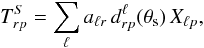 (2)where the index p runs over the Fourier modes in the direction of the rings, and r specifies the index for the cross-ring direction. In Eq. (2), we apply the definition of the Wigner rotation matrix to introduce the real quantity d
 (3)where we choose θ = θs, the constant latitude of the experiment’s spin axis. We also make use of the rotated beam X according to
 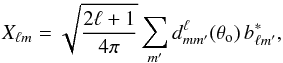 (4)where the bℓm are the expansion coefficients of the beam function in spherical harmonics, and the Wigner small d matrix is evaluated at the opening angle of the scanning circles, θo. We note that this framework allows an exact treatment of arbitrarily shaped beam patterns. The signal covariance matrix
  is then given by
 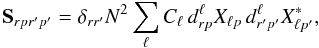 (5)where the Kronecker delta ensures the block diagonal structure of the signal covariance matrix in Fourier space.
After having specified the signal properties, we now quantify the noise correlations. Assuming a stationary Gaussian process, we can describe the noise properties in the TOD domain by a power spectrum P(k). We stress that this ansatz enables the exact treatment of correlated noise, a common systematic effect in real-world experiments. The noise covariance matrix  simplifies to
 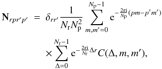 (6)where Nr is the number of rings in the data set, and Np the number of pixels per ring. We have introduced an auxiliary function C(Δ,m,m′), which is defined as
  (7)In analogy to S, we also find the noise covariance matrix N to be block diagonal in Fourier space.
3. Calculating the Fisher matrix on the ring torus
We now propose a strategy for the exact calculation of the Fisher matrix in only calO(N2log N) operations. Given the definition of the Fisher matrix as the covariance of the score function, from Eq. (1), we obtain (Tegmark 1997) ![Mathematical equation: \begin{eqnarray} \label{eq:fisher} F_{\ell_{1} \ell_{2}} &=& - \left \langle \frac{\partial^2 \ln {\cal L}}{\partial C_{\ell_{1}} \partial C_{\ell_{2}}} \right \rangle \nonumber \\ &=& \frac{1}{2} \, \mathrm{tr} \left[ \mathbf{C}^{-1} \mathbf{P}^{\ell_{1}} \mathbf{C}^{-1} \mathbf{P}^{\ell_{2}} \right] , \end{eqnarray}](/articles/aa/full_html/2012/04/aa18985-12/aa18985-12-eq32.png) (8)where C = S + N, and Pℓ = ∂C/∂Cℓ. The evaluation of Eq. (8) in its general form written here takes calO(N3) operations (Borrill 1999).
(8)where C = S + N, and Pℓ = ∂C/∂Cℓ. The evaluation of Eq. (8) in its general form written here takes calO(N3) operations (Borrill 1999).
3.1. Idealized ring-torus scanning strategy
We first consider an idealized experiment as described in the last section. For the calculation of the Fisher matrix, we need to compute the inverse of the covariance matrix, C-1, which can be done brute force in calO(N2) operations owing to its block diagonal structure. The second ingredient, according to Eq. (8), is the derivative of the covariance matrix with respect to the power spectrum coefficients. On the ring torus, we can calculate the derivative for each block r separately as  (9)that is, each block of the matrix is a rank one object and can therefore be written as the outer product of a single vector q. Introducing the decomposition
  , Eq. (8) simplifies considerably to
 ![Mathematical equation: \begin{eqnarray} \label{eq:fisher_torus} F_{\ell_{1} \ell_{2}} &=& \frac{1}{2} \sum_{r} \mathrm{tr} \left[ \mathbf{C}^{-1}_{r} q^{\ell_{1}}_{r} q^{\ell_{1} \, \dagger}_{r} \mathbf{C}^{-1}_{r} q^{\ell_{2}}_{r} q^{\ell_{2} \, \dagger}_{r} \right] \nonumber \\ &=& \frac{1}{2} \sum_{r} \vert q^{\ell_{1} \, \dagger}_{r} \mathbf{C}^{-1}_{r} q^{\ell_{2}}_{r} \vert^2 . \end{eqnarray}](/articles/aa/full_html/2012/04/aa18985-12/aa18985-12-eq40.png) (10)This exact rank-1 representation of the derivative of the signal covariance matrix in the ring-torus Fourier domain is the key ingredient to our fast algorithm. We note that the analogous derivative in the spherical harmonic domain is also block diagonal but with blocks of rank 2ℓ + 1 (Tegmark 1997). We now show how to exploit this low-rank representation.
(10)This exact rank-1 representation of the derivative of the signal covariance matrix in the ring-torus Fourier domain is the key ingredient to our fast algorithm. We note that the analogous derivative in the spherical harmonic domain is also block diagonal but with blocks of rank 2ℓ + 1 (Tegmark 1997). We now show how to exploit this low-rank representation.
For each of the calO(ℓmax) independent blocks of the covariance matrix, we perform the following calculations. We first evaluate the ℓmax matrix-vector products C-1q, at a numerical cost of  . We then accumulate each of the
  entries of the Fisher matrix by a simple vector dot product, with a calO(ℓmax) scaling. The overall time complexity of the algorithm therefore amounts to
  operations.
To confirm the scaling behavior as claimed above, we did a full numerical implementation of the algorithm. In Fig. 1, we show the timings we obtained for different values of ℓmax. The measured runtime clearly follows the predicted time complexity  . The tests were carried out on a cluster of Intel Xenon processors with a 3 GHz clock rate using 256 CPU cores.
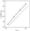 |
Fig. 1 Fast calculation of the Fisher matrix. For several values of ℓmax, we show the measured runtime of our algorithm (filled circles). To guide the eye, we overplot a |

3.2. Generalization beyond ring-torus scans and arbitrary sky coverage
After having outlined the algorithm for the specific case of a simplified scanning strategy, we now discuss how to generalize the results to a generic CMB experiment. To this end, we propose a resampling of the input data to a grid that can be mapped onto the ring torus (e.g., an ECP grid, where θs = θo = π/2). This has the advantage that the simplifying signal covariance properties, as described above, are still fulfilled, i.e. Eq. (9) still holds. Unfortunately, as the grid no longer follows the scanning strategy, the possibility of achieving an exact treatment of asymmetric beams at no additional computational costs is lost. In addition, the noise properties may be more complicated, owing to, e.g., anisotropically distributed observation time, or the presence of a Galactic mask. As a result, an explicit expression for the covariance matrix C may not exist. Luckily, we only have to evaluate products of inverse covariance matrix and sky map. This problem is standard in CMB data analysis, and iterative solvers have been successfully developed for this problem (Smith et al. 2007).
As the block diagonal structure of C is destroyed, we solve  (11)by first finding solutions to the ℓmax equations x = C-1q iteratively, and then contracting the outcome with a simple dot product. Once the calculation has been completed successfully, the resulting Fisher matrix is independent of the pixelization used for the actual computation.
The overall calO(N2) time complexity of the algorithm can be sustained, if the solver scales as  . In the most general case, where the full characterization of the noise properties requires a dense N × N noise covariance matrix, the numerical costs increase to
  operations. Even worse, the memory requirement to store the matrix rises to calO(N2), reaching thousands of terabytes for Planck-sized data.
Luckily, all carefully designed CMB experiments allow either a structured or a sparse representation of the noise covariance matrix. In the presence of an anisotropic yet uncorrelated noise and arbitrary sky coverage, for example, it reduces to a diagonal matrix in a real space representation. This ansatz made an efficient inverse variance weighting of WMAP data possible (Komatsu et al. 2011). Under very general circumstances, the noise covariance can be written in a mixed real-space and time-ordered domain representation, e.g.  , where A is the pointing matrix and NTOD is the noise covariance in the time-ordered domain. For essentially all past and current CMB experiments, the noise is piecewise stationary in the time-ordered domain, which means that NTOD is block-Toeplitz, and the matrix-vector product of N-1 with the data takes
  operations. Since there are at most
  orientations in which a CMB experiment can scan the sky,
  . As a consequence, the calculation of the Fisher matrix in calO(N2log N) operations becomes feasible.
A straightforward treatment of asymmetric beams is only possible if the data grid follows the scanning strategy directly. Although this is not the case in the general setup discussed above, we note that asymmetric beams can be included into the analysis at additional computational costs of  , determined by the azimuthal structure of the beams. For example, the treatment of elliptical Gaussian beams increases the numerical complexity by a factor of four.
4. Discussion and conclusions
The Fisher information matrix is a fundamental quantity in statistics, reflecting the predictive power of the experiment under consideration. Despite its importance, thorough systematic Fisher-matrix-based studies of experiments, designed to measure the CMB power spectrum, have not yet been conducted. The reason for this shortcoming can be found in the associated computational expenses: general algorithms show a time complexity of calO(N3), where N is the number of pixels of the survey, rendering an analysis for state of the art experiments impossible (Borrill 1999).
Here, we have presented a new method for the exact calculation of the Fisher matrix of the CMB power spectrum coefficients in only calO(N2log N) operations. To do so, we first considered experiments with a specific scanning strategy, where the sky is observed on iso-latitude circles. This restriction has allowed us to map the TOD onto the ring torus in order to take advantage of the symmetries of this manifold. We then cast the equation for the CMB likelihood function into Fourier space and found that both the signal and the noise covariance matrices are block diagonal (Wandelt & Hansen 2003). For each block, the derivative of the signal covariance matrix with respect to a single power spectrum coefficient was also found to be a rank one matrix. As a result, we made significant progress in ensuring that the equations to calculate the Fisher matrix exactly simplify, requiring only calO(N2) operations to evaluate.
We then relaxed the assumption of a simplified scanning strategy. If iterative methods allowed us to calculate inverse-variance-weighted sky maps in  operations, we showed that a calO(N2log N) time complexity of our algorithm could be realized. To this end, the data were resampled onto an ECP grid, which is homeomorphic to the ring torus, where the properties of the signal covariance matrix were still simplified. Our fast method is applicable to a very general class of experiments, including, to a good approximation, all CMB data sets taken up to now.
We consider a fast means of calculating the Fisher information matrix for CMB experiments of great importance. This new method not only allows us to study quantitatively the impact of the common systematics of realistic CMB experiments, such as partial sky coverage, asymmetric beams, or correlated noise, on the power spectrum. The Fisher matrix also appears as a normalization factor for unbiased and optimal power spectrum estimators (Tegmark 1997). Since its fast calculation has not been possible, until now, only approximative pseudo-Cℓ estimators have been efficient enough to be applicable to more recent CMB experiments (e.g., Szapudi et al. 2001; Wandelt et al. 2001; Hivon et al. 2002). The new scheme outlined here has the potential to lift this restriction.
For the presentation of our method, we explicitly considered an experiment designed to measure the CMB power spectrum. However, the described framework is general enough to be of value in other fields of application, where the statistical properties of an isotropic signal in spherical geometry are investigated. These applications may include, but are not limited to, the analysis of galaxy angular power spectra (Rimes & Hamilton 2005; Lee & Pen 2008), or weak lensing tomography (Bernstein & Jain 2004; Takada & Jain 2004).
Acknowledgments
B.D.W. was supported by the ANR Chaire d’Excellence and NSF grants AST 07-08849 and AST 09-08902 during this work. F.E. gratefully acknowledges funding by the CNRS. This research was supported in part by the National Science Foundation through XSEDE resources provided by the XSEDE Science Gateways program under grant number TG-AST100029.
References
- Bennett, C. L., Halpern, M., Hinshaw, G., et al. 2003, ApJS, 148, 1 [NASA ADS] [CrossRef] [Google Scholar]
- Bernstein, G., & Jain, B. 2004, ApJ, 600, 17 [NASA ADS] [CrossRef] [Google Scholar]
- Berti, E., Buonanno, A., & Will, C. M. 2005, Phys. Rev. D, 71, 084025 [NASA ADS] [CrossRef] [MathSciNet] [Google Scholar]
- Bond, J. R., Efstathiou, G., & Tegmark, M. 1997, MNRAS, 291, L33 [NASA ADS] [Google Scholar]
- Borrill, J. 1999, Phys. Rev. D, 59, 027302 [NASA ADS] [CrossRef] [Google Scholar]
- Dunkley, J., Hlozek, R., Sievers, J., et al. 2011, ApJ, 739, 52 [NASA ADS] [CrossRef] [Google Scholar]
- Hamilton, A. J. S., & Tegmark, M. 2000, MNRAS, 312, 285 [NASA ADS] [CrossRef] [Google Scholar]
- Hivon, E., Górski, K. M., Netterfield, C. B., et al. 2002, ApJ, 567, 2 [NASA ADS] [CrossRef] [Google Scholar]
- Hu, W., & Tegmark, M. 1999, ApJ, 514, L65 [NASA ADS] [CrossRef] [Google Scholar]
- Jungman, G., Kamionkowski, M., Kosowsky, A., & Spergel, D. N. 1996, Phys. Rev. D, 54, 1332 [NASA ADS] [CrossRef] [Google Scholar]
- Keisler, R., Reichardt, C. L., Aird, K. A., et al. 2011, ApJ, 743, 28 [NASA ADS] [CrossRef] [Google Scholar]
- Kitching, T. D., Taylor, A. N., & Heavens, A. F. 2008, MNRAS, 389, 173 [NASA ADS] [CrossRef] [Google Scholar]
- Komatsu, E., Smith, K. M., Dunkley, J., et al. 2011, ApJS, 192, 18 [NASA ADS] [CrossRef] [Google Scholar]
- Kuo, C. L., Ade, P. A. R., Bock, J. J., et al. 2004, ApJ, 600, 32 [NASA ADS] [CrossRef] [Google Scholar]
- Lee, J., & Pen, U.-L. 2008, ApJ, 686, L1 [NASA ADS] [CrossRef] [Google Scholar]
- Netterfield, C. B., Ade, P. A. R., Bock, J. J., et al. 2002, ApJ, 571, 604 [NASA ADS] [CrossRef] [Google Scholar]
- Perotto, L., Lesgourgues, J., Hannestad, S., Tu, H., & Wong, Y. 2006, J. Cosmol. Astropart. Phys., 10, 13 [Google Scholar]
- Planck Collaboration 2011, A&A, 536, A1 [NASA ADS] [CrossRef] [EDP Sciences] [Google Scholar]
- Rimes, C. D., & Hamilton, A. J. S. 2005, MNRAS, 360, L82 [NASA ADS] [Google Scholar]
- Seo, H.-J., & Eisenstein, D. J. 2003, ApJ, 598, 720 [NASA ADS] [CrossRef] [Google Scholar]
- Smith, K. M., & Zaldarriaga, M. 2011, MNRAS, 417, 2 [NASA ADS] [CrossRef] [Google Scholar]
- Smith, K. M., Zahn, O., & Doré, O. 2007, Phys. Rev. D, 76, 043510 [NASA ADS] [CrossRef] [Google Scholar]
- Smoot, G. F., Bennett, C. L., Kogut, A., et al. 1992, ApJ, 396, L1 [NASA ADS] [CrossRef] [Google Scholar]
- Szapudi, I., Prunet, S., & Colombi, S. 2001, ApJ, 561, L11 [NASA ADS] [CrossRef] [Google Scholar]
- Takada, M., & Jain, B. 2004, MNRAS, 348, 897 [NASA ADS] [CrossRef] [Google Scholar]
- Tegmark, M. 1997, Phys. Rev. D, 55, 5895 [Google Scholar]
- Vallisneri, M. 2008, Phys. Rev. D, 77, 042001 [NASA ADS] [CrossRef] [Google Scholar]
- Wandelt, B. D., & Hansen, F. K. 2003, Phys. Rev. D, 67, 023001 [NASA ADS] [CrossRef] [Google Scholar]
- Wandelt, B. D., Hivon, E., & Górski, K. M. 2001, Phys. Rev. D, 64, 083003 [NASA ADS] [CrossRef] [Google Scholar]
All Figures
|
Fig. 1 Fast calculation of the Fisher matrix. For several values of ℓmax, we show the measured runtime of our algorithm (filled circles). To guide the eye, we overplot a |
| In the text | |
Current usage metrics show cumulative count of Article Views (full-text article views including HTML views, PDF and ePub downloads, according to the available data) and Abstracts Views on Vision4Press platform.
Data correspond to usage on the plateform after 2015. The current usage metrics is available 48-96 hours after online publication and is updated daily on week days.
Initial download of the metrics may take a while.