| Issue |
A&A
Volume 540, April 2012
|
|
|---|---|---|
| Article Number | A115 | |
| Number of page(s) | 7 | |
| Section | Cosmology (including clusters of galaxies) | |
| DOI | https://doi.org/10.1051/0004-6361/201118638 | |
| Published online | 06 April 2012 | |
3D spherical analysis of baryon acoustic oscillations
1 Laboratoire d’Astrophysique, École Polytechnique Fédérale de Lausanne (EPFL), Observatoire de Sauverny, 1290 Versoix, Switzerland
e-mail: This email address is being protected from spambots. You need JavaScript enabled to view it.
2 Laboratoire AIM, UMR CEA-CNRS-Paris 7, Irfu, SAp/SEDI, Service d’Astrophysique, CEA Saclay, 91191 Gif-sur-Yvette Cedex, France
3 Institute for Astronomy, ETH Zürich, Wolfgang Pauli Strasse 27, 8093 Zürich, Switzerland
Received: 13 December 2011
Accepted: 17 January 2012
Abstract
Context. Baryon acoustic oscillations (BAOs) are oscillatory features in the galaxy power spectrum which are used as a standard rod to measure the cosmological expansion. These have been studied in Cartesian space (Fourier or real space) or in spherical harmonic space in thin shells.
Aims. Future wide-field surveys will cover both wide and deep regions of the sky and thus require a simultaneous treatment of the spherical sky and of an extended radial coverage. The spherical Fourier-Bessel (SFB) decomposition is a natural basis for the analysis of fields in this geometry and facilitates the combination of BAO surveys with other cosmological probes readily described in this basis. In this paper, we present a new way to analyse BAOs by studying the BAO wiggles from the SFB power spectrum.
Methods. In SFB space, the power spectrum generally has both a radial (k) and tangential (ℓ) dependence and so do the BAOs. In the deep survey limit and ignoring evolution, the SFB power spectrum is purely radial and reduces to the Cartesian Fourier power spectrum. In the opposite limit of a thin shell, all the information is contained in the tangential modes described by the 2D spherical harmonic power spectrum.
Results. We find that the radialisation of the SFB power spectrum is still a good approximation even when considering an evolving and biased galaxy field with a finite selection function. This effect can be observed by all-sky surveys with depths comparable to current surveys. We also find that the BAOs radialise more rapidly than the full SFB power spectrum.
Conclusions. Our results suggest the first peak of the BAOs in SFB space becomes radial out to ℓ ~ 10 for all-sky surveys with the same depth as SDSS or 2dF, and out to ℓ ~ 70 for an all-sky stage IV survey. Subsequent BAO peaks will also become radial, but for shallow surveys these may be in the non-linear regime. For modes that have become radial, measurements at different ℓ’s are useful in practice to reduce measurement errors.
Key words: methods: observational / cosmology: observations / large-scale structure of Universe / methods: statistical / methods: data analysis
© ESO, 2012
1. Introduction
The study of large scale structure (LSS) with galaxy surveys is a promising tool to study the dark universe (Peacock et al. 2006; Albrecht et al. 2006). Baryon acoustic oscillations (BAOs) are a special feature in the galaxy power spectrum present on scales 100 h-1 Mpc, which are due to oscillations in the coupled baryon-photon fluid before recombination (Sunyaev & Zeldovich 1970; Peebles & Yu 1970; Eisenstein et al. 2005; Seo & Eisenstein 2003, 2007). The BAOs are considered a powerful cosmological tool as the BAO scale acts as a standard ruler with which to probe cosmic expansion both in the radial and tangential directions.
BAOs were first detected by Eisenstein et al. (2005) in SDSS data (Adelman-McCarthy et al. 2008) and later with 2dF galaxies (Colless et al. 2003; Cole et al. 2005) and finally with both surveys (Percival et al. 2007b), though others suggest current data cannot currently probe the BAO scale sufficiently (Cabré & Gaztañaga 2011).
Until now, BAOs have been studied in Cartesian space, either in Fourier space (Seo & Eisenstein 2003, 2007), or in real space (Eisenstein et al. 2005; Xu et al. 2010; Slosar et al. 2009), and in 2D spherical harmonic space on thin spherical shells (Dolney et al. 2006). These descriptions use different information and therefore have different constraining power for cosmological parameters (Rassat et al. 2008).
Future wide-field BAO surveys will, however, cover both large and deep areas of the sky, and thus require a simultaneous treatment of the spherical sky geometry and of extended radial coverage. The spherical Fourier-Bessel (SFB) decomposition is a natural basis for the analysis of fields in this geometry. The SFB analysis is powerful as it uses a coordinate system in which the radial selection function and physical effects are naturally described. Moreover, this description facilitates the combination of BAO surveys with other cosmological probes which are readily described in the SFB decomposition such as the smooth power spectrum and redshift space distortions (Heavens & Taylor 1995; Fisher et al. 1995b; Percival et al. 2004; Erdoğdu et al. 2006a,b), weak lensing (Heavens 2003; Castro et al. 2005; Kitching et al. 2008), and the integrated Sachs-Wolfe effect (ISW, Shapiro et al. 2011). Studying BAOs from wide-field surveys with an SFB expansion, is therefore natural both for the geometry considered, and for unifying the treatment with the other probes.
In Sect. 2 we first review the general decomposition of a 3D field in SFB space and introduce the concept of radialisation when the field is statistically isotropic and homogeneous. In Sect. 3.1, we introduce a new way to consider the BAOs, by studying the baryon wiggles in SFB space, in a similar way as in Fourier space, while in Sect. 3.2 we discuss the radialisation of BAOs in SFB space in the context of existing and future surveys. In Sect. 4 we present our conclusions.
2. 3D spherical Fourier-Bessel (SFB) expansion
2.1. Expansion of an homogeneous and isotropic field
Let us consider a field f(r) at time t, where r = (r,θ,ϕ) in spherical polar coordinates. In practice, this field may represent the galaxy or mass density (or overdensity) in the universe. In a flat geometry, the field can be decomposed in the 3D SFB basis set, which is complete and orthonormal, as 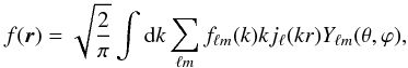 (1)where jℓ(x) are spherical Bessel functions of the first kind, Yℓm(θ,ϕ) are spherical harmonics, ℓ and m are multipole moments and k is the wavenumber. The inverse relation is
 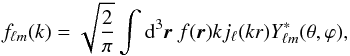 (2)where we use the same conventions as Leistedt et al. (2012) and Castro et al. (2005) (see also Heavens & Taylor 1995; Fisher et al. 1995b, who use a different convention and basis set).
This decomposition can be viewed as the spherical polar coordinate analogue to the Fourier decomposition in Cartesian coordinates given by  The 3D SFB power spectrum Cℓ(k) of the field f(r) is given by the the 2-point function of the SFB coefficients fℓm(k) which can be written as
  (5)when the field is statistically isotropic and homogeneous (hereafter, the SIH condition). Similarly and in the same condition, the Fourier power spectrum P(k) is implicitly defined by
  (6)These two power spectra are related by (see for e.g., Fisher et al. 1995b; Castro et al. 2005):
  (7)Thus, the SFB power spectrum Cℓ(k) is independent of the multipole ℓ, and thus only has a radial (k) dependence. This remarkable yet recondite fact is only true if the field fulfills the SIH condition.
In the following subsections, we discuss the impact of the (partial) violation of this condition in practice and the implication for the measurements of BAO in SFB analysis.
2.2. Finite surveys
In practice, a cosmological field, such as the galaxy density field, will only be partially observed due the finite survey volume. In this case the observed field fobs(r) can be described by  (8)where φ(r) is the radial selection function of the survey, and f(r) is assumed to fulfill the SIH condition for now (we will address the effect of bias and evolution in Sect. 2.3). The observed field fobs(r) is thus no longer homogeneous because of the radial the selection function. There may also be a tangential selection function to account for regions of missing data, but we assume here that the data is available on the full sky. For convenience, the selection function is normalised as
  (9)where V is a characteristic volume of the survey chosen such that φ → 1 as V → ∞, such that
  (10)In this case, the homogeneity condition (SIH) is no longer valid in the radial direction and the observed 2-point function can be written as
  (11)where the observed SFB power spectrum
  depends this time on ℓ, k and k′, as opposed to only on ℓ and k as in Eq. (5). It can be shown that it can be expressed as
 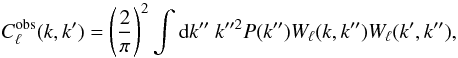 (12)where P(k) is defined in Eq. (6) and the window function Wℓ(k,k′) is defined as
  (13)In practice, tends to fall off rapidly away from the diagonal k = k′ and we will often only compute
  defined by:
  (14)We next evaluate the window function and the observed power spectrum for three special cases for the selection function.
2.2.1. Gaussian selection function
As a first example, let us consider a Gaussian selection function defined as  (15)where r0 is a radius parameter and the normalisation obeys Eq. (9) (with
  ). In this case, the window function can be integrated analytically (using relation 6.633.2 of Gradshteyn et al. 2000), and Eq. (13) becomes:
 ![Mathematical equation: \begin{equation} W_\ell(k,k') = \frac{\pi r_0^2}{4}\sqrt{\frac{k}{k'}}\exp \left[ -r_0^2 \frac{k^2 + k'^2}{4}\right] I_{\ell+\frac{1}{2}} \left(\frac{r_0^2 kk'}{2}\right), \label{eq:analytic:window} \end{equation}](/articles/aa/full_html/2012/04/aa18638-11/aa18638-11-eq41.png) (16)where Iν(x) is the modified Bessel function of the first kind. This analytical form considerably facilitates the evaluation of Eq. (12) (see Sect. A for a way to numerically calculate the above equation for large arguments of Iν(x)).
(16)where Iν(x) is the modified Bessel function of the first kind. This analytical form considerably facilitates the evaluation of Eq. (12) (see Sect. A for a way to numerically calculate the above equation for large arguments of Iν(x)).
2.2.2. Radial limit
In the case where the radial selection function corresponds to full radial coverage (i.e. φ(r) = 1,∀r), the window function becomes  (17)Inserting this expression into Eq. (12), we recover Eq. (7), namely
  (18)meaning that the 3D spherical spectrum is only dependent on radial coordinate k, as discussed above.
As we show in Appendix A, this limit can also be obtained by taking the limit r0 → ∞ for the Gaussian weight function of Eq. (15) and is achieved in practice when the condition (see Eq. (A.4))  (19)is satisfied. We refer to this as the radialisation of the field and discuss this more in Sect. 3.
2.2.3. Tangential Limit
In the other extreme case, the radial selection function covers only a thin shell of the field at a distance r ∗  (20)where the normalisation of Eq. (9) was chosen with
  . Equation (12) then becomes
 ![Mathematical equation: \begin{eqnarray} C^{\rm obs}_\ell(k,k')&=& \left(\frac{2}{\pi}\right)^2kk' j_\ell(kr_*)j_\ell(k'r_*)\nonumber\\ &&\times \int {\rd} k'' k''^2 P(k'')\left[r_*^3 j_\ell(k''r_*)\right]^2.\label{eq:clk3D} \end{eqnarray}](/articles/aa/full_html/2012/04/aa18638-11/aa18638-11-eq51.png) (21)This can be related to the statistics of the 2D projected field
(21)This can be related to the statistics of the 2D projected field  (22)whose spherical harmonic decomposition is given by
 and whose 2D spherical harmonic power spectrum
  is defined by
  (25)This power spectrum is related to the 3D Fourier space power spectrum P(k) by:
 ![Mathematical equation: \begin{equation} C^{\rm 2D}_\ell =\frac{2}{\pi}\int {\rd} kk^2P(k)\left[W^{\rm 2D}_\ell(k)\right]^2, \end{equation}](/articles/aa/full_html/2012/04/aa18638-11/aa18638-11-eq56.png) (26)where the 2D window function
(26)where the 2D window function  is given by
  (27)Note that due to our choice of normalisation for φ(r) in Eq. (9), has units of volume.
In the case of a thin-shell selection function (Eq. (20)), this reduces to ![Mathematical equation: \begin{equation} C^{\rm 2D}_\ell=\frac{2}{\pi}\int {\rd} k k^2 P(k) \left[r^3_* j_\ell(kr_*)\right]^2\label{eq:cl2D}. \end{equation}](/articles/aa/full_html/2012/04/aa18638-11/aa18638-11-eq59.png) (28)Thus, the SFB power spectrum (Eq. (21)) is simply related to the 2D spherical harmonic power spectrum1 by
(28)Thus, the SFB power spectrum (Eq. (21)) is simply related to the 2D spherical harmonic power spectrum1 by  (29)The term kk′jℓ(kr ∗ )jℓ(k′r ∗ ) is a geometric factor which does not depend on the field f. Thus, in this case, all the information in the 3D SFB spectrum Cℓ(k,k′) is contained in the 2D power spectrum , i.e. depends solely on ℓ.
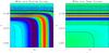 |
Fig. 1 Ratio |
2.3. Evolution and bias
For a realistic galaxy field, the SIH condition will not be met due to the radial evolution of the field from the growth of structure and redshift dependent bias.
For a biased and evolving field in the linear regime, the galaxy power spectrum Pevol(k,r) will have an explicit distance dependence:  (30)where the term b(r) is the linear bias, assumed to be scale-independent, D(r) is the growth factor and P(k) = P(k,r = 0) is the matter power spectrum at r = z = 0. The linear approximation will hold up to a redshift-dependent scale kmax(z). In the standard cosmological model, we find kmax(z = 0) ≃ 0.12 h Mpc-1 (i.e., before the second BAO peak) and kmax(z = 2) ≃ 0.25 h Mpc-1.
For the realistic galaxy field, an approximation for the spherical 3D power spectrum for the galaxy field is still given by Eq. (12), but the window function will incorporate the linear growth and bias functions as  (31)
(31)
3. Application to baryon acoustic oscillations
3.1. SFB Analysis of BAOs
The matter power spectrum in Eq. (12) includes the physical effects of baryons, which create oscillations in Fourier space (Sunyaev & Zeldovich 1970; Peebles & Yu 1970; Seo & Eisenstein 2003; Eisenstein et al. 2005; Seo & Eisenstein 2007). These BAOs can be isolated by considering the ratio RP(k) in Fourier space:  (32)where Pb(k) is the galaxy (or matter) power spectrum including the physical effect of BAOs, and Pnob(k) is broad band or “smooth” part of the galaxy (or matter) power spectrum. In linear theory the growth and bias terms cancel out so that Eq. (32) is independent of z. These oscillations can also be probed in 2D spherical harmonic space (Dolney et al. 2006). We are interested here to see if they can similarly be probed in SFB space as well.
In SFB space, we consider the ratio  given by:
  (33)where similarly to Fourier space,
  is the diagonal SFB power spectrum (Eq. (14)) including the physical effects of baryons and
  is the “smooth” part of the SFB power spectrum. These are calculated by using Pb(k) or Pnob(k) instead of P(k) in Eq. (12) and then considering Eq. (14). The SFB decomposition suggests that the BAOs can manifest themselves in both k and ℓ space.
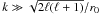
In Fig. 1, we plot for two wide-field galaxy surveys with a shallow (left) and deep (right) galaxy Gaussian selection functions with r0 = 100 h-1 Mpc, and 1400 h-1 Mpc respectively (see Sect. 2.2.1). We chose a fiducial concordance cosmology with Ωm = 0.25, ΩDE = 0.75, Ωb = 0.045, w0 = −0.95, wa = 0.0, h = 0.70, σ8 = 0.80, ns = 1 and no running spectral index. We consider both to be “realistic” surveys, i.e. with evolution due to growth taken into account and a linear galaxy bias (taken as  ), using Eq. (31) for the window function.
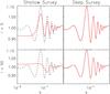 |
Fig. 2 Slices in |
In the LHS of Fig. 1 (narrow survey), the BAOs depend on both k and ℓ modes, illustrating that the wiggles can be measured simultaneously in the ℓ and k directions, which is the first result of this paper.
However, in the RHS of Fig. 1 (wide survey), the BAOs appear to have only a radial (k) dependence, except at very large physical scales (k < 0.01 h Mpc-1), where the dependence is both radial and tangential. This is a practical illustration of Eq. (18) (see also Eq. (A.5)). This can be understood as tangential modes being attenuated due to mode-cancelling along the line of sight – the attenuation becomes important when the selection function spans a wide redshift range. We refer to this effect as the radialisation of the power spectrum, where we have used the baryonic wiggles to probe the radialisation. We discuss the radialisation limit in more detail in Sects. 3.2 and 4.
One of the important results of Fig. 1 is that the radial limit is still reached even when evolution (growth and bias) of the field are considered. This can only be considered numerically since there is no analytic solution to Eq. (31) due to the inclusion of the growth and bias terms. We test this again with strongly evolving values of the galaxy bias, e.g.  , where n = −10,2, and find this still has little effect on the radialisation of . The growth values for standard concordance cosmology do not seem to have an effect on reaching the radialisation limit.
3.2. Radialisation limit
We are interested in quantifying the effect of the radialisation on the BAOs themselves. In Fig. 2, we consider slices in ℓ and k through in order to investigate how rapidly the limit in Eq. (18) is reached. The black (dashed) lines in Fig. 2 correspond to RP(k) (which are independent of ℓ and of the survey selection function) and the red (solid) lines correspond to for different slices in ℓ space and for narrow (LHS) and wide (RHS) selection functions. As the survey selection function is widened, we find that: 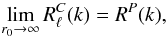 (34)i.e. tends towards the oscillations in RP(k), not only in phase, but also in amplitude. This is noticeable in Fig. 1: the amplitude of the first peak for example is higher for the deep survey ( > 9%) than for the shallow survey ( < 8%). This is another check of Eq. (7).
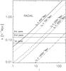 |
Fig. 3 Radialisation limit as defined by Eq. (19) (diagonal lines) for Gaussian surveys (Eq. (15)) with r0 = 40,70,200,300,1400 h-1 Mpc, i.e. roughly corresponding to the following surveys: IRAS (zmean ~ 0.015), 2MRS (zmean ~ 0.03), SDSS (zmean ~ 0.10), 2dF (zmean ~ 0.15), and a stage IV survey (zmean ~ 0.80). Information above the diagonal line is in the radial limit. We overplot the physical scales corresponding to the first three BAO peaks for comparison. |
Equation (19) gives us an analytic way to study the limit where we can expect the SFB power spectrum to behave radially. In Fig. 3, we plot the lines corresponding to the radial limit in (k,ℓ) space for different surveys with Gaussian distributions (Eq. (15)) corresponding to r0 = 40,70,200,300,1100 [h-1 Mpc] . We have chosen these values as they correspond roughly to the following surveys (for the chosen fiducial survey): IRAS (zmean ~ 0.015, Fisher et al. 1995a; Strauss et al. 1992), 2MRS (2 MASS All-Sky Redshift Survey, zmean ~ 0.03, Huchra et al. 2012), SDSS (Sloan Digital Sky Survey, zmean ~ 0.10, Adelman-McCarthy et al. 2008), 2dF (2 degree Field, zmean ~ 0.15, Colless et al. 2003) and a Stage IV galaxy survey (zmean ~ 0.80, Albrecht et al. 2006). Note that, in principle, these surveys would have to be all-sky to obey the radialisation limits plotted in Fig. 3.
The area above each diagonal line corresponds the radial limit, i.e. where the radialisation has taken place and Eq. (18) holds. We overplot the radial scales corresponding to the first three peaks of the BAOs to show how these will be probed for different survey depths.
By comparing the diagonal lines in Fig. 3 with the BAO “turnover” (i.e. the ℓ-dependent k-scale at which the BAOs switch from being mostly tangential to mostly radial) in Fig. 1, we notice however that the BAOs seem to become radial before the full SFB power spectrum does, especially for large ℓ. This surprising effect, further motivates the use of the SFB analysis for BAOs.
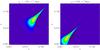 |
Fig. A.1 Window function Wℓ(k,k′) for the Gaussian selection function with for ℓ = 3 and r0 = 100 h-1 Mpc (left) and r0 = 1400 h-1 Mpc (right). As the selection function parameter r0 becomes larger (i.e., increasing the redshift coverage from zmed ~ 0.05 to zmed ~ 0.8), the window function tends towards |

4. Conclusion
In this paper, we have presented a new way to study BAOs using a SFB decomposition of a wide-field deep galaxy survey. The BAO signal in SFB space can be studied by considering the ratio of the SFB power spectrum with wiggles  to the smooth SFB power spectrum
  , similarly to what is done in Fourier space. In this decomposition, BAOs can be observed simultaneously in both the radial (k) and tangential (ℓ) modes.
For a field which is statistically isotropic and homogeneous (SIH), the SFB power spectrum is purely radial, i.e. independent of tangential modes, and reduces to the Cartesian Fourier power spectrum. In the other extreme limit where the field is in a thin shell, we showed that all the SFB information is contained in the tangential modes and is simply related to the 2D spherical harmonic power spectrum.
Considering the practical case where the field is observed with a radial selection function (thus partially violating the SIH condition), we find that the radial limit can still be reached for selection functions covering a large radial range (see Appendix A), which we refer to as the radialisation of the power spectrum. The radialisation will be limited to a region in (ℓ,k) space corresponding to  , where r0 parameterises the radial selection function. We find that radialisation is a good approximation for these modes even when evolution due to growth and bias are considered, both of which can be considered as a further violation of the SIH condition. To study this limit, we have derived an analytic solution to the window function of a non-evolving, unbiased galaxy field when the radial selection function is a Gaussian in r centered on the observer (Eq. (16)).
We also find the BAOs considered in SFB space radialise as the survey depth is increased, meaning both the phase and amplitude of the BAOs tend towards the Fourier space ratio RP(k). This means that BAOs for a wide-field shallow survey have smaller amplitude and are spread across the (ℓ,k) space, while BAOs for a wide-field deep survey have a larger amplitude and are confined to the radial modes (Figs. 1 and 2).
We study the radial limit analytically (Fig. 3) and find that it can in principle be observed (for a limited ℓ-range and for small physical scales) with all-sky surveys with current surveys depths or for future stage-IV surveys. This suggest that the first BAO peak becomes radial up to ℓ ~ 10 for an all-sky survey with similar depth to SDSS or 2dF, and up to ℓ ~ 70 for an all-sky stage IV survey. In practice though, the radialisation might be observable to even higher ℓ since we observe that the BAOs radialise more rapidly than the full SFB power spectrum, especially at large ℓ. Subsequent BAO peaks also become radial for large values of ℓ and for shallower surveys, though these may be already be in the non-linear regime. For modes that have become radial, measurements at different ℓ’s are useful in practice, to reduce measurement errors due to cosmic variance and shot noise.
We note that we have ignored redshift-space distortions in our analysis though the prescription for these in SFB space is well known (see for e.g., Heavens & Taylor 1995). These distortions may affect the radialisation as they will introduce mode-mixing, albeit with a distinct signature and are readily described in the SFB basis. Further ℓ-mode mixing will occur for incomplete sky coverage, which can be corrected for using the mask geometry.
Equation (29) is conceptually different from Eq. (B3) in Kitching et al. (2011): the former is an exact solution for a thin shell, while the latter uses the Limber approximation.
Acknowledgments
The authors are grateful to Pirin Erdoğdu, Alan Heavens, Ofer Lahav, François Lanusse, Boris Leistedt and Adam Amara for useful discussions about SFB decompositions. The SFB calculations use the discrete spherical Bessel transform (DSBT) presented in Lanusse et al. (2012) and the authors are grateful to François Lanusse for help implementing this. We extended iCosmo2 software for our calculations (Refregier et al. 2011). This research is in part supported by the Swiss National Science Foundation (SNSF).
References
- Adelman-McCarthy, J. K., Agüeros, M. A., Allam, S. S., et al. 2008, ApJS, 175, 297 [NASA ADS] [CrossRef] [Google Scholar]
- Albrecht, A., Bernstein, G., Cahn, R., et al. 2006 [arXiv:astro-ph/0609591] [Google Scholar]
- Cabré, A., & Gaztañaga, E. 2011, MNRAS, 412, L98 [NASA ADS] [Google Scholar]
- Castro, P. G., Heavens, A. F., & Kitching, T. D. 2005, Phys. Rev. D, 72, 023516 [NASA ADS] [CrossRef] [Google Scholar]
- Cole, S., Percival, W. J., Peacock, J. A., et al. 2005, MNRAS, 362, 505 [NASA ADS] [CrossRef] [Google Scholar]
- Colless, M., Peterson, B. A., Jackson, C., et al. 2003 [arXiv:astro-ph/0306581] [Google Scholar]
- Dolney, D., Jain, B., & Takada, M. 2006, MNRAS, 366, 884 [NASA ADS] [Google Scholar]
- Eisenstein, D. J., Zehavi, I., Hogg, D. W., et al. 2005, APJ, 633, 560 [Google Scholar]
- Erdoğdu, P., Huchra, J. P., Lahav, O., et al. 2006a, MNRAS, 368, 1515 [Google Scholar]
- Erdoğdu, P., Lahav, O., Huchra, J. P., et al. 2006b, MNRAS, 373, 45 [NASA ADS] [CrossRef] [Google Scholar]
- Fisher, K. B., Huchra, J. P., Strauss, M. A., et al. 1995a, ApJS, 100, 69 [NASA ADS] [CrossRef] [Google Scholar]
- Fisher, K. B., Lahav, O., Hoffman, Y., Lynden-Bell, D., & Zaroubi, S. 1995b, MNRAS, 272, 885 [NASA ADS] [Google Scholar]
- Gradshteyn, I. S., Ryzhik, I. M., Jeffrey, A., & Zwillinger, D. 2000, Table of Integrals, Series, and Products, 6th edn. (Academic Press) [Google Scholar]
- Heavens, A. 2003, MNRAS, 343, 1327 [NASA ADS] [CrossRef] [Google Scholar]
- Heavens, A. F., & Taylor, A. N. 1995, MNRAS, 275, 483 [NASA ADS] [Google Scholar]
- Huchra, J. P., Macri, L. M., Masters, K. L., et al. 2012, ApJS, 199, 26 [NASA ADS] [CrossRef] [Google Scholar]
- Kitching, T. D., Taylor, A. N., & Heavens, A. F. 2008, MNRAS, 389, 173 [NASA ADS] [CrossRef] [Google Scholar]
- Kitching, T. D., Heavens, A. F., & Miller, L. 2011, MNRAS, 413, 2923 [NASA ADS] [CrossRef] [Google Scholar]
- Lanusse, F., Rassat, A., & Starck, J.-L. 2012, A&A, 540, A92 [NASA ADS] [CrossRef] [EDP Sciences] [Google Scholar]
- Leistedt, B., Rassat, A., Refregier, A., & Starck, J.-L. 2012, A&A, 540, A60 [NASA ADS] [CrossRef] [EDP Sciences] [Google Scholar]
- Peacock, J. A., Schneider, P., Efstathiou, G., et al. 2006, ESA-ESO Working Group on Fundamental Cosmology, Tech. Rep. [Google Scholar]
- Peebles, P. J. E., & Yu, J. T. 1970, ApJ, 162, 815 [NASA ADS] [CrossRef] [Google Scholar]
- Percival, W. J., Burkey, D., Heavens, A., et al. 2004, MNRAS, 353, 1201 [NASA ADS] [CrossRef] [Google Scholar]
- Percival, W. J., Cole, S., Eisenstein, D. J., et al. 2007b, MNRAS, 381, 1053 [NASA ADS] [CrossRef] [MathSciNet] [Google Scholar]
- Rassat, A., Amara, A., Amendola, L., et al. 2008, unpublished [arXiv:0810.0003] [Google Scholar]
- Refregier, A., Amara, A., Kitching, T. D., & Rassat, A. 2011, A&A, 528, A33 [NASA ADS] [CrossRef] [EDP Sciences] [Google Scholar]
- Seo, H.-J., & Eisenstein, D. J. 2003, APJ, 598, 720 [NASA ADS] [CrossRef] [Google Scholar]
- Seo, H.-J., & Eisenstein, D. J. 2007, APJ, 665, 14 [CrossRef] [Google Scholar]
- Shapiro, C., Crittenden, R. G., & Percival, W. J. 2011, MNRAS, submitted [arXiv:1109.1981] [Google Scholar]
- Slosar, A., Ho, S., White, M., & Louis, T. 2009, J. Cosmol. Astropart. Phys., 10, 19 [NASA ADS] [CrossRef] [Google Scholar]
- Strauss, M. A., Huchra, J. P., Davis, M., et al. 1992, ApJS, 83, 29 [NASA ADS] [CrossRef] [EDP Sciences] [Google Scholar]
- Sunyaev, R. A., & Zeldovich, Y. B. 1970, Ap&SS, 7, 3 [NASA ADS] [Google Scholar]
- Xu, X., White, M., Padmanabhan, N., et al. 2010, ApJ, 718, 1224 [NASA ADS] [CrossRef] [Google Scholar]
Appendix A: Radial limit for a Gaussian selection function
As shown in Sect. 2.2.1, when the galaxy selection is Gaussian, i.e. φ(r) = e − (r/r0)2 , it is the galaxy selection function (Eq. (13)) reduces to ![Mathematical equation: \appendix \setcounter{section}{1} \begin{equation} W_\ell(k,k')=\frac{\pi r_0^2}{4}\sqrt{\frac{k}{k'}}\exp\left[-r_0^2\frac{k^2+k'^2}{4}\right]I_{\ell+\frac{1}{2}}\left( \frac{r_0^2k k'}{2}\right), \end{equation}](/articles/aa/full_html/2012/04/aa18638-11/aa18638-11-eq130.png) (A.1)where Iν(x) is the modified Bessel function of the first kind. For numerical reasons, it is often useful to evaluate the exponentially scaled modified Bessel function of the first kind
(A.1)where Iν(x) is the modified Bessel function of the first kind. For numerical reasons, it is often useful to evaluate the exponentially scaled modified Bessel function of the first kind  instead of Iν(x), in which case it is useful to re-write the above equation as:
 ![Mathematical equation: \appendix \setcounter{section}{1} \begin{equation} W_\ell(k,k')=\frac{\pi r_0^2}{4}\sqrt{\frac{k}{k'}}\exp\left[-r_0^2 \left( \frac{k-k'}{2}\right)^2 \right] \tilde{I}_{\ell+\frac{1}{2}} \left(\frac{r_0^2k k'}{2}\right)\cdot \end{equation}](/articles/aa/full_html/2012/04/aa18638-11/aa18638-11-eq132.png) (A.2)Figure A.1 shows the window function for two values of r0, ℓ = 3 as a function of k,k′. As r0 becomes large, it can be seen that the window function tends towards a delta function
(A.2)Figure A.1 shows the window function for two values of r0, ℓ = 3 as a function of k,k′. As r0 becomes large, it can be seen that the window function tends towards a delta function  .
.
To study this limit more precisely, we use the asymptotic form for the modified Bessel function  for x ≫ | α2 − 1/4 | , which gives
 ![Mathematical equation: \appendix \setcounter{section}{1} \begin{equation} W_{\ell}(k,k') \simeq \frac{\sqrt{\pi}}{4} \frac{r_0}{k'} \exp\left[-r_0^2 \left( \frac{k-k'}{2}\right)^2 \right], \end{equation}](/articles/aa/full_html/2012/04/aa18638-11/aa18638-11-eq137.png) (A.3)in the limit where
(A.3)in the limit where  , or approximately,
  (A.4)Using the definition of a Dirac delta function, namely ∫dx h(x)δ(x − x0) = h(x0) for an arbitrary function h(x), the window function becomes, in the limit r0 → ∞,
  (A.5)in agreement with Eq. (17) for the radial case discussed in Sect. 2.2.2. Thus, if the condition of Eq. (A.4) holds, the power spectrum becomes radial (i.e. independent of ℓ) and equal to Cℓ(k)δ(k − k′) = P(k)δ(k − k′) as in Eq. (18).
All Figures
|
Fig. 1 Ratio |
| In the text | |
|
Fig. 2 Slices in |
| In the text | |
|
Fig. 3 Radialisation limit as defined by Eq. (19) (diagonal lines) for Gaussian surveys (Eq. (15)) with r0 = 40,70,200,300,1400 h-1 Mpc, i.e. roughly corresponding to the following surveys: IRAS (zmean ~ 0.015), 2MRS (zmean ~ 0.03), SDSS (zmean ~ 0.10), 2dF (zmean ~ 0.15), and a stage IV survey (zmean ~ 0.80). Information above the diagonal line is in the radial limit. We overplot the physical scales corresponding to the first three BAO peaks for comparison. |
| In the text | |
|
Fig. A.1 Window function Wℓ(k,k′) for the Gaussian selection function with for ℓ = 3 and r0 = 100 h-1 Mpc (left) and r0 = 1400 h-1 Mpc (right). As the selection function parameter r0 becomes larger (i.e., increasing the redshift coverage from zmed ~ 0.05 to zmed ~ 0.8), the window function tends towards |
| In the text | |
Current usage metrics show cumulative count of Article Views (full-text article views including HTML views, PDF and ePub downloads, according to the available data) and Abstracts Views on Vision4Press platform.
Data correspond to usage on the plateform after 2015. The current usage metrics is available 48-96 hours after online publication and is updated daily on week days.
Initial download of the metrics may take a while.