| Issue |
A&A
Volume 540, April 2012
|
|
|---|---|---|
| Article Number | A30 | |
| Number of page(s) | 10 | |
| Section | Planets and planetary systems | |
| DOI | https://doi.org/10.1051/0004-6361/201118551 | |
| Published online | 20 March 2012 | |
An improved model of the Edgeworth-Kuiper debris disk
Astrophysikalisches Institut, Friedrich-Schiller-Universität Jena, Schillergäßchen 2–3, 07745 Jena, Germany
e-mail: This email address is being protected from spambots. You need JavaScript enabled to view it.
Received: 30 November 2011
Accepted: 7 February 2012
Abstract
In contrast to all other debris disks, where the dust can be seen via an infrared excess over the stellar photosphere, the dust emission of the Edgeworth-Kuiper belt (EKB) eludes remote detection because of the strong foreground emission of the zodiacal cloud. We accessed the expected EKB dust disk properties by modeling. We treated the debiased population of the known trans-Neptunian objects (TNOs) as parent bodies and generated the dust with our collisional code. The resulting dust distributions were modified to take into account the influence of gravitational scattering and resonance trapping by planets on migrating dust grains as well as the effect of sublimation. A difficulty with the modeling is that the amount and distribution of dust are largely determined by sub-kilometer-sized bodies. These are directly unobservable, and their properties cannot be accessed by collisional modeling, because objects larger than (10...60) m in the present-day EKB are not in a collisional equilibrium. To place additional constraints, we used in-situ measurements of the New Horizons spacecraft within 20 AU. We show that to sustain a dust disk consistent with these measurements, the TNO population has to have a break in the size distribution at s ≲ 70 km. However, even this still leaves us with several models that all correctly reproduce nearly constant dust impact rates in the region of giant planet orbits and do not violate the constraints from the non-detection of the EKB dust thermal emission by the COBE spacecraft. The modeled EKB dust disks, which conform to the observational constraints, can either be transport-dominated or intermediate between the transport-dominated and collision-dominated regime. The in-plane optical depth of such disks is τ∥(r > 10 AU) ~ 10-6 and their fractional luminosity is fd ~ 10-7. Planets and sublimation are found to have little effect on dust impact fluxes and dust thermal emission. The spectral energy distribution of an EKB analog as seen from 10 pc distance peaks at wavelengths of (40...50) μm at F ≈ 0.5 mJy, which is less than 1% of the photospheric flux at those wavelengths. Therefore, EKB analogs cannot be detected with present-day instruments such as Herschel/PACS.
Key words: methods: numerical / infrared: planetary systems / Kuiper belt: general / planet-disk interactions / interplanetary medium
© ESO, 2012
1. Introduction
The Edgeworth-Kuiper belt (EKB) with its presumed collisional debris is the main reservoir of small bodies and dust in the solar system and constitutes the most prominent part of the solar system’s debris disk. However, the EKB dust has not been unambiguously detected so far. The observational evidence for the EKB dust is limited to scarce in-situ detections of dust in the outer solar system by a few spacecraft, partly with uncalibrated “chance detectors” (Gurnett et al. 1997; Landgraf et al. 2002; Poppe et al. 2010). In addition, there are rough upper limits on the amount of dust from the non-detection of thermal emission of the EKB dust on a bright zodiacal light foreground (Backman et al. 1995). Given the lack of observational data, one can only access the properties of the EKB dust by modeling. This modeling takes the known EKB populations to be parent bodies for dust and uses collisional models to generate dust distributions (Stern 1995, 1996; Vitense et al. 2010; Kuchner & Stark 2010).
In our previous paper (Vitense et al. 2010), we took the current database of known trans-Neptunian objects (TNOs) and employed a new algorithm to eliminate the inclination and the distance selection effects in the known TNO populations and derived expected parameters of the “true” EKB. Treating the debiased populations of EKB objects as dust parent bodies, we then produced their dust disk with our collisional code.
The main goal of this paper is to improve the model by Vitense et al. (2010) in several important respects:
-
I.
Although we do not modify the debiasing algorithm and staywith the same “true” EKB as defined in Vitenseet al. (2010), we re-address thequestion of how the size distribution in the present-day EKB thatwe only know down to sizes of ~10 km should be extrapolated down to the dust sizes. Accordingly, we present the new collisional code runs that make different assumptions about the amount of objects smaller than ~10 km in the current EKB. Besides, these new runs include a more realistic material composition (a mixture of ice and astrosilicate in equal fractions) and an accurate handling of the cross-section of dust grains. This is done in Sect. 2.
-
II.
We estimate the influence of planets (resonant trapping and gravitational scattering) (Sect. 3).
-
III.
We include the possible effect of ice sublimation (Sect. 4).
-
IV.
We finally make a detailed comparison of the model with the spacecraft in-situ measurements, including the first results of New Horizons (Poppe et al. 2010; Han et al. 2011), as well as with the thermal emission constraints by COBE (Greaves & Wyatt 2010, and references therein). This is done in Sects. 5 and 6.
Our results are summarized in Sect. 7 and discussed in Sect. 8.
2. The dust production model
2.1. The size distribution in the EKB
We start with general remarks about the size distribution in the EKB and its evolution since the early phases of the solar system formation. Because it is not known how planetesimals in the solar nebula have formed, their primordial size distribution is unclear. In standard coagulation scenarios, the bottom-up growth of planetesimals could have resulted in a broad size distribution (e.g., Kenyon & Bromley 2008), with a more or less constant slope across all sizes up to roughly the size of Pluto. Alternatively, local gravitational instability in turbulent disks would have produced predominantly big (~100 km) planetesimals (Johansen et al. 2006, 2007; Cuzzi et al. 2008; Morbidelli et al. 2009), implying a knee in the size distribution at these sizes, which is indicated by several observations (Bernstein et al. 2004; Fuentes & Holman 2008; Fraser & Kavelaars 2009; Fuentes et al. 2009). Next, according to the Nice model (Gomes et al. 2005; Levison et al. 2008; Morbidelli 2010), the primordial Kuiper belt was compact (between 15 and 35 AU) and massive (~50 Earth masses). With these parameters, the EKBOs with sizes up to hundreds of kilometers would have been collisionally processed by the time of the late heavy bombardment (LHB) in ≈ 800 Myr from the birth of the solar system. Therefore, the size distribution consisted of two parts before the LHB. Objects smaller than hundreds of km had a size distribution set by their collisional evolution in the early massive EKB, whereas larger objects retained a primordial distribution set by their formation process. The LHB has then resulted in a dynamical depletion of the EKB, which was obviously size-independent (Wyatt et al. 2011). As a result, the entire size distribution must have been pushed down, retaining its shape. During the LHB, the EKB has reduced its original mass by a factor of ~1000 (Levison et al. 2008) and expanded to its present position. Both the reduction of mass and the increase of distance to the Sun have drastically prolonged the collisional lifetime of the EKBOs of any given size. As a result, only objects smaller than about a hundred of meters in radius (more accurate values will be obtained below, see Fig. 3) experienced full collisional reprocessing during the subsequent 3.8 Gyr. We conclude that the size distribution in the EKB after the LHB, and in the present-day EKB, is likely to consist of three parts. Objects smaller than a hundred meters must currently reside in a collisonal equilibrium, those with radii between a hundred meters and hundreds of kilometers inherit the collisional steady-state of the massive and compact belt of the pre-LHB stage, and the largest EKBOs still retain a primordial size distribution from their accretion phase.
2.2. Setup of the collisional simulations
To obtain the dust distributions in the present-day EKB, which is the goal of this paper, we used our collisional code ACE (Analysis of Collisional Evolution) (Krivov et al. 2000, 2005; Krivov et al. 2006, 2008; Löhne et al. 2008; Müller et al. 2010). This code simulates the evolution of orbiting and colliding solids, using a mesh of sizes s, pericentric distances  , and eccentricities e of objects as phase space variables. It includes the effects of stellar gravity, direct radiation pressure, Poynting-Robertson force, stellar wind, and several collisional outcomes (sticking, rebounding, cratering, and disruption), and collisional damping.
If we were able to set an initial size and orbital distribution of bodies (i.e., the one after the completion of the LHB) in a reasonable way, we could simply run the code over 3.8 Gyr to see which dust distribution it yields. Setting the initial distribution at largest EKBOs, i.e. the third of the three parts of the entire size distribution described above, is straightforward. Because the distribution of these objects remains nearly unaltered since the LHB, their initial distribution should be nearly the same as the current one. Accordingly, we populated the ACE bins with the debiased population of known EKBOs, as described in Vitense et al. (2010).
However, we do not know the second part of the distribution, at least for objects between a hundred meters and ~10 km, where no or very few EKBOs have been discovered. Given the lack of information on these objects, we chose to extrapolate the size distribution to smaller objects with a power law dN ∝ s − qds. The slope q is unknown, so we explored the following possibilities (thin lines in Fig. 1):
-
1.
Run “d” (“Dohnanyi extrapolation”). We assume the classicalDohnanyi (1969) law with q = 3.5. This extrapolation is similar to the one used in Vitense et al. (2010).
-
2.
Run “f” (“flat extrapolation”). We assume q = 3.0 for s < 10 km. Run “f” can be treated as a rough proxy for a break in the size distribution at a few tens of kilometers reported in the literature: q ≈ 1.9 (Fraser & Kavelaars 2009), q ≈ 2.0 (Fuentes et al. 2009) and q ≈ 2.5 (Fuentes & Holman 2008). Keeping in mind that the observed TNOs include several populations, and that the knowledge of scattered objects is particularly poor (Vitense et al. 2010), we made an additional run “fCKB” identical to “f”, but without the scattered objects.
-
3.
Run “n” (“no extrapolation”). Here, we refrain from any extrapolation, assuming that the system was devoid of smaller objects initially. This formally corresponds to q → − ∞.
To complete the specification of the initial conditions for the ACE simulations, we have yet to set the orbital distributions of the objects with s ≲ 10 km. Because there are no relevant observational data, we simply assumed that these objects inherit the pericentric distance and the eccentricity from their parent bodies. This means that for every object that resides in a bin  , the bins
  are populated with (sl / si)1 − q (l < i) objects (assuming logarithmic size bins).
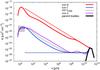 |
Fig. 1 Size distributions in different collisional runs. Thin lines are initial distributions, while thick ones correspond to an advanced state of collisional evolution. Note that the initial size distribution of the “n” run coincides with the debiased population of TNOs. A is the cross-section density per size decade at a distance of 40 AU. Note that A = const. (i.e. horizontal lines) corresponds to a size distribution with q = 3, where different-sized objects equally contribute to the cross-section. The gray shaded rectangle is a rough approximation of the particle dust flux given by New Horizons translated into the cross-section density and distances of the EKB. |
As a minimum grain radius, we chose 0.4 μm and set size ratios of the adjacent bins of 1.5 for dust sizes and 2.3 for the largest TNOs. To cover the heliocentric distances from 4 AU to 400 AU we used a logarithmically spaced pericenter grid with 21 bins as well as a linearly spaced eccentricity grid between −1.5 and 1.5. Note that negative eccentricities correspond to “anomalous” hyperbolic orbits, which are open outward from the star and are attained by smallest dust grains with a radiation pressure to gravity ratio β > 1 (Krivov et al. 2006). To make sure that this fairly coarse grid yields sufficiently accurate results, we made another “n” run with a finer, more extended grid with a minimum grain radius of 0.3 μm with size ratios of the adjacent bins of 1.25 for dust sizes and 1.58 for the largest TNOs, 41 pericenter bins and eccentricity bins between −5 and 5. We found that our coarse grid leads to almost the same results as the fine grid model.
As material, we assumed a mixture of 50% ice (Warren 1984) and 50% astrosilicate (Laor & Draine 1993) with a bulk density of 2.35 g cm-3. The optical constants of the mixture were computed with the Bruggeman mixing rule and the absorption coefficients with a standard Mie algorithm. The values of other parameters, e.g. the critical fragmentation energy, were the same as in Vitense et al. (2010).
2.3. Results of the collisional simulations
All extrapolations described above are rather arbitrary, and the last one is obviously unrealistic. A natural question is then, which of the models, and after which timestep, will deliver the distributions that match the actual distributions of the EKB material the best. We start with the integration time. Each of the runs was let continue as long as needed to reach a collisional equilibrium at smaller sizes, but not too long to preserve the initial distribution of larger objects. A boundary between “smaller” and “larger” sizes was arbitrarily set to s ~ 1 km. We considered “collisional equilibrium” to have been reached once the shape of the size distribution stopped changing. To meet these criteria in the “n” run, we had to let the system evolve much longer than the age of the Universe. Of course, this “modeling time” should not be misinterpreted as the physical time of the EKB evolution. This was merely the time needed for the population of large bodies to generate a sufficient amount of smaller debris down to dust sizes.
The results obtained over the integration interval chosen in this way are shown in Figs. 1–3 with thick lines. These three figures show the size distribution, the radial profile of the normal geometrical optical depth, and the collisional lifetime of the objects, respectively. We note that at an earlier stage of evolution the cross-section density and the normal optical depth would be lower, and the lifetime of dust grains longer, while a later stage of evolution would lead to more dust and therefore to a higher cross-section density and optical depth and reduced lifetime of the particles.
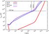 |
Fig. 3 Lifetimes of dust grains and parent bodies for the same ACE runs and time instants as in Fig. 1. Particles below the 3.8 Gyr line are in a collisional equilibrium after the LHB. A steep rise in the lifetime at s ~ 300 m corresponds to the strength-gravity transition of the critical disruption energy. |
But which of the models, “d”, “f”, of “n” – if any – matches the actual dust distribution in the present-day EKB best? The only way to answer this question is to compute the observables for each of the simulations and compare them with in-situ spacecraft measurements and thermal emission constraints. Although an in-depth analysis of the data is deferred to Sect. 5, we now take a first quick look. The gray shaded rectangle in Fig. 1 is a rough approximation of the dust flux data collected by New Horizons, translated into the cross-section density and extrapolated to the distance of the classical EKB. A comparison with the evolved curves demonstrates that the “d” run is far too dusty. It cannot reach an evolutionary stage that would be consistent with the measurements (and with the upper limit from the non-detection of the thermal emission). Therefore we conclude that a straightforward extrapolation from debiased EKBOs to dust sizes has to be ruled out. Consequently, we showed here, with a completely different type of argument, that a break in the size distribution has to be present in the EKB, as found from the analysis of TNO observations (Fuentes & Holman 2008; Fraser & Kavelaars 2009; Fuentes et al. 2009).
How about the other runs? Both the “f” and the “n” runs are consistent with the observational data; we will confirm this in Sect. 5 by a more thorough analysis. Thus – unfortunately – we cannot constrain the size distribution of EKBOs more tightly. Nor can we say which of the dust distributions, the one of the “f” run or the “n” run, can be expected in the EKB, although the shape of the curves in these runs is different. (The only common feature shared by all the curves is an abrupt drop at ≈ 0.5 μm, which is the limit below which the grains are swiftly removed from the system by radiation pressure.) We now come to an analysis of these differences.
The size distribution in the “d” run, which we rejected because it violated the of observational constraints, is typical of a collision-dominated disk. At all sizes, the dust transport is less efficient than the collisional grinding, and the cross-section density peaks just above the blowout limit (Krivov et al. 2006; Thébault & Augereau 2007). This is also confirmed by the radial profile shown in Fig. 2. The outer slope of ≈ 1.2 agrees well with an approximate analytic solution for a collision-dominated disk that predicts a slope of ≈ 1.5 (Strubbe & Chiang 2006). Also, there is a clear decrease of the optical depth toward the star, caused by collisional elimination of the particles. Since we can rule out this extrapolation, additional results for the “d” run are presented but not discussed anymore. As mentioned above, the “d” run is essentially the same as the run in Vitense et al. (2010) (made for the expected EKB, with the Poynting-Robertson effect included), therefore we refer to our previous work for a detailed analysis of the “d” run. As shown here, this run fails to describe the actual present-day EKB in the solar system. Nevertheless, the results and conclusions presented in Vitense et al. (2010) would still be valid for an EKB analog in which all objects down to kilometer in size are in collisional equilibrium.
The size distribution in the “n” run is different. It shows a broad maximum at ~100 μm, which indicates that particles smaller than that are transported inward from the dense part of the disk before they are lost to collisions (Wyatt et al. 2011). The inner part of the radial profile in Fig. 2 is nearly constant, and the outer one reveals a steeper slope of ≈3.0, as predicted analytically for a transport-dominated disk (≈2.5, Strubbe & Chiang2006). Note that the outer profiles are generated by particles in a narrow range of sizes around the blowout limit. The coarse size grid in our models therefore limits the accuracy with which we can reproduce these slopes.
The “f” run seems to be intermediate. Although the maximum in the size distribution is broader than in the “d” run, it still resembles the curves typical of collision-dominated disks. However, the profile of the normal optical depth (Fig. 2) stays nearly constant inside the main belt, which is typical of transport-dominated disks (e.g. Wyatt 2005).
Figures 1–3 also present the results of the additional “fCKB” run, from which we excluded scattered objects as dust parent bodies. Figure 1 shows, somewhat unexpectedly, that the results of “f” and “fCKB” runs differ from each other: the dust disk in the latter turns out to be transport-dominated, similar to the “n” run. The question is why. This is not because dropping the scattered objects just reduces the amount of material in the EKB, resulting in reduced collisional rates. A test simulation in which we artificially augmented the mass of the classical EKB to the total mass of the expected EKB brought qualitatively the same results as the “fCKB” run. Instead, the answer can be found in the method of extrapolation. As explained before, we filled the (s,q,e)-bins with our debiased population of EKBOs and extrapolated toward smaller sizes with a power law into the same (q,e)-bins. That means that we transfered the high eccentricities of the large scattered objects to all smaller ones. Although higher eccentricities do not lead to higher collisional rates (see Krivov et al. 2007, discussion after their Eq. (17)), they increase the relative velocities, making collisions more disruptive. In the “f” run a large amount of s < 10 μm particles is produced, leading to a higher number and cross-section density for these particles, which in turn leads to a higher collisional rate and a shorter collisional lifetime for larger particles (Fig. 3). Without the eccentric orbits of scattered objects (“fCKB” run), the relative velocities are moderate, collisions are less disruptive and fewer small particles are produced. Therefore, destruction of larger grains becomes less efficient, leading to a prolonged collisional lifetime.
The above discussion demonstrates that it remains unclear whether the EKB dust disk is transport- or collision-dominated. It is most likely that it is either transport-dominated or intermediate between a collision- and transport-dominated disk. However, in all the runs considered, the inner part of the dust disk (inside the classical EKB) has a nearly constant radial profile of the optical depth of τ⊥ ~ 1 × 10⁻⁷ (Fig. 2). (For comparison, the in-plane optical depth for r > 10 AU is τ∥ = 1...2 × 10-6.) This suggests that collisions in the inner part of the disk can be neglected. This justifies that in this section we first simulated a completely planet- and sublimation-free EKB and will include the effects of planetary scattering and sublimation below, in Sects. 3 and 4.
Figure 3 shows the mean collisional lifetimes averaged over all distances for the same ACE runs at the same time instants. Note that the collisional lifetime in the main belt is much shorter than the average one because the density there is much higher and therefore collisions are more frequent. The horizontal line represents a lifetime of 3.8 Gyr, which is the time elapsed after the LHB. All grains below this line are in a collisional equilibrium in the present EKB. For all simulations this size is just about (10...60) m. The distribution of all objects larger than that equilibrium size was set before the LHB and cannot be constrained with our collisional model.
3. Influence of planets
Giant planets interact gravitationally with dust in the outer solar system. On the one hand, the grains drifting inward by the Poynting-Robertson (P-R) drag (Burns et al. 1979) can be captured by planets into outer mean-motion resonances (e.g. Liou & Zook 1999; Moro-Martín & Malhotra 2002, 2003, 2005; Kuchner & Stark 2010). On the other hand, the grains that cross the planet’s orbit can be scattered. Both effects are able to modify the size and spatial distribution of dust in the disk. In this section, we investigate the efficiency of capturing and scattering.
3.1. Resonant trapping
Mustill & Wyatt (2011) developed a general formalism to calculate the capture probability of a particle into the first- and second-order resonances with a planet. Their theory is valid for any convergent differential migration of the particle and the planet (for instance, if the particle is drifting inward and the planet is migrating outward). Their results are presented in terms of the generalized momentum J and a dimensionless drift rate Ḃ ( in their paper).
The generalized momentum is related to the orbital eccentricity of the particle reaching the resonance location, e, while the dimensionless drift rate Ḃ can be expressed through the differential change rate of the particle’s semimajor axis, ȧres, and the semimajor axis itself, ares. Below, we make estimates for the 3:2 resonance with Neptune. Using Eqs. (3) and (4) of Mustill & Wyatt (2011), we find the following conversion relations: 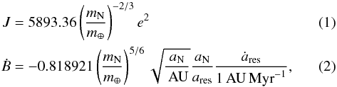 where m⊕ and mN denote the masses of Earth and Neptune, respectively, and aN is the semimajor axis of the Neptune orbit.
We now assume that ȧres is caused by P-R drag (Wyatt & Whipple 1950) ![Mathematical equation: \begin{eqnarray} \dot{a}_\text{res} &=& - 1.3\frac{\beta}{c} \frac{G M_{\odot}}{a_\text{res}} \frac{2 + 3 e^2}{(1-e^2)^{3/2}} \nonumber\\ &=& -815\frac{\beta}{a_\text{res}[\text{AU}]}\frac{2 + 3 e^2}{(1-e^2)^{3/2}}\frac{\AU}{\Myr} , \label{dot a_res} \end{eqnarray}](/articles/aa/full_html/2012/04/aa18551-11/aa18551-11-eq81.png) (3)where the prefactor 1.3 accounts for the enhancement of P-R drag by solar wind drag (Burns et al. 1979) and β is the radiation pressure to gravity ratio for the particle. The enhancement by solar wind drag is included in the subsequent analysis but we will call it P-R drag for brevity. The β-ratio not only controls the drift rate, it also reduces the effective solar mass felt by the particle by a factor of (1 − β). This affects the resonance location, so that ares reads
(3)where the prefactor 1.3 accounts for the enhancement of P-R drag by solar wind drag (Burns et al. 1979) and β is the radiation pressure to gravity ratio for the particle. The enhancement by solar wind drag is included in the subsequent analysis but we will call it P-R drag for brevity. The β-ratio not only controls the drift rate, it also reduces the effective solar mass felt by the particle by a factor of (1 − β). This affects the resonance location, so that ares reads ![Mathematical equation: \begin{equation} a_\text{res} = a_\text{N}\sqrt[3]{1-\beta} \left(3/2\right)^{2/3}. \label{a_res} \end{equation}](/articles/aa/full_html/2012/04/aa18551-11/aa18551-11-eq85.png) (4)Inserting Eqs. (3) and (4) into Eq. (2), the latter takes the form
(4)Inserting Eqs. (3) and (4) into Eq. (2), the latter takes the form 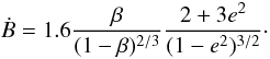 (5)Using the capture probabilities as functions of J and Ḃ from Mustill & Wyatt (2011) and applying Eqs. (1) and (5), we computed the probabilities as functions of e and β (or equivalently, particle radius s). The results for the 3:2 resonance with Neptune are shown in Fig. 4. Although capturing for grains s > 0.6 μm and e < 0.03 seems unavoidable, it is not obvious what is the fraction of particles of those sizes that will actually have such low eccentricities. The reason is that small particles, when released from parent bodies in nearly-circular orbits, are sent by radiation pressure into large and highly-eccentric orbits. Subsequently, drag forces reduce the semimajor axes and eccentricities of the grains. Yet, it is not clear how low the eccentricities will be by the time when the grains will have reached the resonance location.
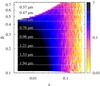 |
Fig. 4 Capture probability of a single particle with given β and e at the location of the 3:2 resonance with Neptune. |
To find this out, we first consider parent bodies with elements ap and ep and compute the initial semimajor axis ai and the eccentricity ei of a grain upon release. To this end, we use Eqs. (19)–(20) of Krivov et al. (2006), in which we neglect the mass of the projectile compared to the mass of the target, i.e. the parent body, and assume that ejection occurs at the pericenter of the parent body orbit: 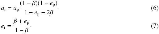 Subsequently, the P-R drag will decrease ai and ei. Denoting by ef the final eccentricity – i.e. the one the grain will have at the location of a resonance, ares = af – and using the dependence of ȧ on ė as given in Wyatt & Whipple (1950)
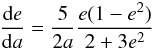 (8)leads to
 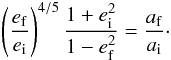 (9)As an example, a plutino with ap ≈ 39 AU and ep = 0.1 will release a β = 0.3 particle into an orbit with ai = 82 AU and ei = 0.57. The 3:2 resonance with Neptune for this particle is located at ares ≈ 35 AU. At that location, the grain will have ef = 0.13.
 |
Fig. 5 Capture probability of a β particle released by a parent body for the 3:2 resonance with Neptune. ep = 0.6 represents the population of scattered objects. Note that all particles above the horizontal lines have initial eccentricites of e > 1 and will be removed from the system (Eq. (7)). |
With Eqs. (6)–(9) and the data of Mustill & Wyatt (2011) it is possible to calculate the capture probability for each resonance and particle size for given ap and ep. As a word of caution, we note that the actual dust dynamics can be more complicated. One complication is that the initial semimajor axis (Eq. (6)) for sufficiently small particles is often so large that the grain has to pass several other resonances before it reaches the 3:2 one. At these resonances, particles with high migration rates and low eccentricities will experience an eccentricity jump when they are not captured. As a result, our model will underestimate the final eccentricity at the 3:2 resonance and so overestimate the capture probability. Slow migration rates and low eccentricities will result in the opposite effect – an eccentricity decrease and a probability increase – so an underestimation of the capture probability is also possible (Mustill & Wyatt 2011). A detailed modeling of this problem is beyond the scope of this paper.
Figure 5 shows the probability of capture into the 3:2 resonance with Neptune. The probability is the highest for ep = 0, but even then it does not exceed ≈ 20% for dust grains below 2 μm when released from classical EKBOs. Increasing the eccentricity of the EKBOs and decreasing the grain size reduces the capturing efficiency. For ep = 0.6, which can be considered representative for scattered-disk objects, the capturing probability is only a few per cent. For ep = 0.1 (typical classical EKBOs) and s ~ 1 μm (slightly above the threshold of the New Horizons dust detector), the trapping probability is still below 10%. Given these results, resonant capturing can be considered unimportant for the purposes of this paper and will be neglected.
3.2. Gravitational scattering
Because P-R drag continuously decreases the particle’s distance from the Sun, the grain will eventually reach the orbit of a planet. As this happens, the grain can either fall onto the planet, be scattered, or pass the planet without interaction. In the first two cases the particle will be lost. To determine the surviving fraction, we used a numerical code that calculates the orbital evolution of a single particle, taking into account the gravity of one planet and the P-R effect. For each β-value listed in Table 1 (these are the same values as used in our collisional simulations) we started 10 000 particles, with an EKB-like a,e,i distribution taken from the upper panel of Fig. 5 from Vitense et al. (2010). A particle was counted as a survivor as soon as its apocentric distance became shorter than the pericentric distance of the planet.
The results are listed in Table 1 for Neptune, Uranus and Saturn. As expected, the surviving rate decreases for larger grains with lower migration rates. For Neptune and Uranus the ejection rate is negligible and will not alter the dust flux significantly (Sect. 5). However, Saturn ejects nearly half of the dust grains. As we will see in Sect. 5, Saturn’s influence is important for the explanation of the in-situ measurements, but all three planets have little effect on the thermal emission of the EKB dust (Sect. 6).
β values and corresponding sizes, masses, and surviving rates for particles passing Neptune, Uranus, and Saturn.
As shown in the previous section, the EKB dust disk is transport-dominated for small particles, which means that collisions play a minor role. Therefore, gravitational scattering can simply be implemented by multiplying the distribution obtained in the collisional simulation by the surviving rates for the corresponding particle sizes and distances.
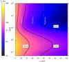 |
Fig. 6 Temperatures of the dirty-ice particles for different distances. The solid lines correspond to 100 K, 75 K and 50 K. Sublimation occurs at Tsubl = 100 K. Sublimation distance increases with decreasing size because the emission efficiency of small grains is lower, which makes them hotter. |
4. Influence of sublimation
When drifting inward, dust grains will not only suffer interaction with planets, but they will also be heated up because of the decreasing distance to the Sun. Our dust particles are composed of “dirty ice” (50% ice and 50% astrosilicate in volume). Their icy part sublimates at ≈ 100 K (Kobayashi et al. 2008, 2009, 2012). Since the EKB dust disk is radially optically thin, the temperature of a dust grain is determined by the energy balance between the absorption of incident solar radiation and the thermal emission of the grain. We neglected the latent heat of sublimation because its contribution is minor (Kobayashi et al. 2008). The sublimation distance rsubl, where the temperature of a particle reaches 100 K, depends on its size. If the particles are larger than λ / (2π), where λ is the peak wavelength of emission, the absorption and emission cross-sections are approximately the same as the geometrical one, and these particles can be assumed to be blackbody radiators. Since for T = 100 K the maximum is at λ ~ 30 μm, this is the case for grains with s > 5 μm. Temperatures of smaller particles are obtained by solving the thermal balance equation (see, e.g., Krivov et al. 2008). Figure 6 shows the resulting temperatures for different sizes and distances, with three isotherms overplotted. The leftmost one corresponds to 100 K. Empirically we can approximate the dependence of the sublimation distance (in AU) on the size (in micrometers) by  (10)We note that this function does not have a physical meaning and is only needed to implement sublimation into our model.
The outcome of sublimation depends on the structure of icy grains. If a single icy particle is an aggregate of small grains, each having β ≳ 0.5, the resulting grains will be blown out and therefore no grains should be present inside rsubl. However, if the constituent monomers have β ≲ 0.5, the number density of grains inside rsubl will increase. Since both is inconsistent with the dust flux measured by spacecraft, a single icy grain is likely to contain a single core of refractory material covered with an ice mantle (Kobayashi et al. 2010). For our dirty-ice grains sublimation will result in a 100% silicate particle that has half of the volume of the original particle. The radius of the resulting particle is simply ![Mathematical equation: \begin{equation} s_\text{silicate} = \sqrt[3]{0.5}s_\text{icy}, \end{equation}](/articles/aa/full_html/2012/04/aa18551-11/aa18551-11-eq153.png) (11)and the mass is given by
(11)and the mass is given by  (12)with ρicy = 2.35 g cm-3 being the bulk density of the dirty ice and ρsilicate = 3.35 g cm-3 of the astrosilicate. The typical sizes and β-values of the particles before and after sublimation are given in Table 2 together with their sublimation distances.
We now discuss how sublimation affects the distribution of dust. The particles born through collisions in the Edgeworth-Kuiper belt have eccentricities roughly comparable to their β values (Eq. (7)). Although damped by P-R drag, their eccentricities in the sublimation zone are typically higher than 0.05. Particles with e > 0.05 will experience a rapid sublimation without pile-up and dust ring formation (Kobayashi-et-al-2009, cf. Burns et al. 1979, their Fig. 8). Next, although sublimation in our model does not eliminate the particles and accordingly preserves their number, it reduces their spatial number density. This is because the number density of particles is inversely proportional to their drift rates in the steady state. Because ȧ ∝ β, the increase of β due to sublimation lessens the number density of particles. Based on Table 2, the change is estimated to be only about 20%, see Fig. 7 below. However, with in-situ dust detectors measuring only grains above a certain threshold, the observable dust flux decreases more strongly.
If we assume that the orbital changes due to the change in size and therefore changing interaction with the stellar radiation are small, we can implement sublimation into our collisional results the same way as gravitational scattering by simply correcting sizes and cross-section- and mass density for the affected bins. Since planetary scattering and sublimation are independent processes, the order of implementation does not matter.
Sizes and β-values before and after sublimation and the corresponding sublimation distances.
5. Comparison with spacecraft measurements
The Student Dust Counter on-board the New Horizons spacecraft is capable of detecting impacts of grains with 10-12 g < m < 10-9 g and can distinguish grain masses apart by a factor of 2 between 0.5 μm < s < 5 μm (Horányi et al. 2008). The first results from Poppe et al. (2010) indicate particle fluxes of up to 1.56 × 10⁻⁴ m-2 s-1. The results of Han et al. (2011) show a slight increase of the flux for r > 15 AU. The particle flux can be calculated via  (13)with m being the mass of the particle, n the number density per logarithmic mass and vrel the relative velocity between the spacecraft and the particle. The first two values are a direct output of our simulation. The relative velocity was assumed to be vrel = 15.54 km s-1, according to the official New Horizons web page1. Based on the results of Sects. 2–4, we calculated the dust fluxes for the EKB dust disk unaffected by planets and sublimation, the one with planets and the one with planets and sublimation. Although the separate contributions of planets and sublimation are rather low, their combination can alter the dust flux by up to a factor of three, in which Saturn plays the most important role. In Fig. 7 the results of run “f” are shown. The proper evolutionary state of the simulation (i.e., timestep) was chosen in the following way. As seen in Fig. 7, the black solid line can be assumed to be a constant for r < 20 AU. With this assumption we fitted the New Horizons data from Poppe et al. (2010) and Han et al. (2011) by a constant line to
  and searched for the timestep that agrees with the model best.
According to Gurnett et al. (1997), the Voyager 1 and 2 plasma wave instruments, which acted as “chance” dust detectors, have a mass threshold of m > 1.2 × 10⁻¹¹ g, which is one order of magnitude higher than for the New Horizons dust counter. Accordingly, we rescaled the Voyager data to the New Horizons threshold, with the power law slope of q = − 1 obtained in our simulation for the corresponding masses (Fig. 1) at 40 AU. Because the instruments aboard Voyager I and II were neither designed to detect dust impacts nor calibrated for this purpose and traversed the outer solar system in highly inclined orbits, their dust measurements should be compared with our model with great caution.
Simulations f, fCKB, and n were treated the same way. Since for the particle sizes in question (s < 5 μm) all modeled disks are transport-dominated, the results do not differ much from each other and lead approximately to the same fits as for the “f” run. Therefore these results are not shown in Fig. 7.
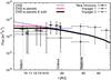 |
Fig. 7 Simulated particle flux compared with in-situ measurements by New Horizons and Voyager 1 and 2. The solid black line takes into account planets and sublimation and represents our best fit to the data taken from Poppe et al. (2010), Han et al. (2011) and Gurnett et al. (1997). The dotted and dashed lines show the dust flux for the unperturbed EKB and after planetary scattering without sublimation, respectively. |
6. Thermal emission constraints
To calculate thermal emission of dust in the EKB, we computed the photospheric spectrum of the Sun using the NextGen models (Hauschildt et al. 1999). The equilibrium dust temperatures were obtained by the procedure of Krivov et al. (2008). As in the collisional simulations, we adopted the “dirty ice” consisting of equal volume fractions of ice (Warren 1984) and astrosilicate (Laor & Draine 1993). As explained in Sect. 4, the sublimation distance depends on the particle size. Therefore we divided the EKB into six sub-rings to handle the different emission properties of the dirty ice and pure astrosilicate (Table 3).
The EKB divided into six sub-rings: material composition together with the sizes and distances for which that composition was adopted.
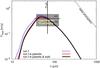 |
Fig. 8 Spectral energy distribution of the EKB including planets and sublimation (solid black line), without sublimation (dashed red line), and for an unperturbed EKB (dottted blue line). All curves are based on the same run (“f”) and the same time instant as in Fig. 7. |
To place our EKB in the context of extrasolar debris disks, we now consider the EKB dust disk as if it were viewed from outside. The final spectral energy distribution (SED) of the EKB dust disk, as seen from a reference distance of 10 pc, is shown in Fig. 8. The influence of planets and sublimation does not significantly alter the shape, peak position, and height. The SED, corrected for planets and sublimation, peaks at 40−50 μm with a maximum thermal emission flux of ≈0.5 mJy, which amounts to ≈ 0.5% of the photospheric flux at that wavelength. The predicted flux drops to ≈0.4 mJy at 70 μm and to ≈0.2 mJy at 100 μm. The fractional luminosity of the modeled EKB dust disk, after applying corrections for planets and sublimation, is fd = 1.2 × 10⁻⁷.
Our results are consistent with the upper limit that is placed by non-detection of the EKB dust emission at 70 μm with the COBE spacecraft. That limit amounts to 1 ± 0.5% of the solar photospheric flux (Greaves & Wyatt 2010) and is shown by the dark gray box in Fig. 8.
Would EKB analogs around nearby stars be detectable, for example, with the PACS instrument (Poglitsch et al. 2010) of the Herschel Space Observatory (Pilbratt et al. 2010)? The sensitivity of the PACS instrument at 70 μm is 4.7 mJy in 1h integration time at a 5σ uncertainty level2. This is about a factor of 10 above the calculated SED flux of 0.4 mJy at 70 μm. This factor would increase even more when taking into account additional background noise and photospheric flux uncertainties. We conclude that the detection of an exact analog of the EKB with the present-day instruments is impossible. An apparent contradiction to Vitense et al. (2010), who concluded that Herschel/PACS should be able to detect an ≈ 2MEKB analog, traces back mainly to a different extrapolation method from parent bodies to smallest grains.
7. Conclusions
The purpose of this paper was to develop a self-consistent model of the EKB debris disk. To accomplish this task we used the debiased population of EKBOs as described in Vitense et al. (2010). Treating this population as dust parent bodies, we generated their dust disk with our collisional code. We draw the following conclusions:
-
1.
We have shown that sub-kilometer-sized EKBOs largelydetermine the amount and distribution of dust in the outer solarsystem. However, these are far too small to be directly detected atpresent in TNO surveys, and their properties cannot be accessedby collisional modeling, because they are not in a collisionalequilibrium. Therefore, an extrapolation from observable TNOstoward smaller sizes is necessary.
-
2.
A straightforward extrapolation for the as yet unknown objects (s ≲ 10 km) with a classical Dohnanyi law can be ruled out. In that case, the amount of dust would be so large that its thermal emission would have been detected by the COBE spacecraft. Therefore, the distribution of these objects should be flatter. In other words, a break in the size distribution at several tens of kilometers has to be present.
-
3.
Different extrapolation methods that are consistent with the measurements reveal the EKB either as a transport-dominated debris disk or to be intermediate between the collision-dominated and transport-dominated regimes. Depending on the extrapolation method, we found the present-day EKB to be in collisional equilibrium for objects s < (10...60) m.
-
4.
Using the results of Mustill & Wyatt (2011), we estimated the effect of resonance trapping of planets. The capturing rate of the dust grains that are either detectable with in-situ measurements by spacecraft or contribute to measurable thermal emission turned out to be <10% in most cases and not to exceed <20% even for the largest grains considered. Accordingly, resonance trapping should have a negligible effect on dust impact rates and dust thermal emission, given the typical accuracy of the dust measurements.
-
5.
Gravitational scattering of dust grains by planets was investigated numerically. Scattering can modify the particle flux in the Saturn-Uranus region (8 AU < r < 15 AU) by about a factor of two and has little effect on thermal emission of dust.
-
6.
Likewise, sublimation can reduce the particle flux by approximately a factor of two and does not affect the thermal emission fluxes perceptibly.
-
7.
We calibrated our model with the in-situ measurements of the New Horizons dust counter (Poppe et al. 2010; Han et al. 2011) by fitting our results to the data points and can reproduce the nearly constant particle flux of 3 × 10⁻⁴ m-2 s-1. The corresponding production rate of dust inside the EKB amounts to 2 × 10⁶ g s-1, consistent with previous estimates (e.g. Yamamoto & Mukai 1998; Landgraf et al. 2002; Han et al. 2011). In a steady-state collisional cascade (which we assume), the “dust production rate” is the same as the “dust loss rate”. Consequently, the result means that 2 tons of dust per second leave the system by inward transport and through ejection as blowout grains.
-
8.
The spectral energy distribution of an EKB analog, seen from a distance of 10 pc, would peak at 40−50 μm with a maximum flux of 0.5 mJy. This is consistent with the upper limit that is placed by non-detection of thermal emission from the EKB dust as it would be viewed from outside at 70 μm by the COBE spacecraft. The fractional luminosity of the EKB was calculated to be fd = 1.2 × 10⁻⁷. The in-plane optical depth for r > 10 AU is set by our model to 2 × 10⁻⁶. Although the Herschel/PACS instrument successfully detects debris disks at similar fractional luminosity levels as the EKB (Eiroa et al. 2010, 2011), these are all larger and therefore colder. Their thermal emission peaks at wavelengths longward of 100 μm, where the stellar photosphere is dimmer. The detection of an exact EKB analog even with PACS would not be possible.
8. Discussion
Like every model, ours rests on many assumptions and is not free of uncertainties. Here we discuss some of them.
-
1.
Material composition. Compared to Vitenseet al. (2010), who appliedgeometric optics in calculating the radiation pressure, we nowconsistently used a more realistic material composition in bothcollisional and thermal emission calculations. Nevertheless, weassumed many parameters of solids – bulkdensity, shape, porosity, tensile strength, andothers – to be the same across the entire size range,from Pluto-sized TNOs down to dust. This assumption isobviously unrealistic.
-
2.
The role of sub-kilometer-sized EKBOs. Since little is known about EKBOs smaller than a few tens of kilometers, but these largely control the amount and distribution of dust in the outer solar system, an extrapolation from observable TNOs towards smaller sizes is necessary. The question is what kind of extrapolation is reasonable. If the parent bodies pass on their orbital elements to their children and grand-children, then the EKB should comprise a huge amount of meter- and sub-kilometer-sized objects in highly eccentric orbits, stemming from scattered EKBOs. This would make collisions more disruptive and alter the size distribution of dust. The resulting size distribution would be dominated by the smallest dust grains, just above the radiation pressure blowout limit. If, in contrast, the meter- and sub-kilometer-sized objects have moderate eccentricities, the peak of the cross-section in the size distribution would be broader and shifted to larger grains. To distinguish between these possibilities, one needs more information about the amount and distribution of sub-kilometer objects. Accurate measurements of sizes and orbital elements of dust grains in the outer solar system in the future would also help.
-
3.
Break in the size distribution of EKBOs. Our model shows that a break in the size distribution at tens of kilometers, as reported in the recent literature, is necessary. Otherwise the EKB dust disk would be too dusty, violating the available observational constraints. If such a break is present in other debris disks as well, then the total mass of parent bodies should be higher than usually inferred in the debris disk studies.
-
4.
Planetary scattering and sublimation. If planetary scattering and/or sublimation is more efficient than assumed in our model, the amount of dust grains that reach the Saturn-Uranus region of the solar system would be smaller. To stay consistent with the in-situ measurements, one would have to compensate higher scattering rates and/or more efficient sublimation by higher dust production rates in the EKB. However, this would lead to a higher thermal emission flux, which would contradict the non-detection of thermal emission by COBE.
http://pluto.jhuapl.edu/mission/whereis_nh.php (Last accessed on 2 September 2011).
http://herschel.esac.esa.int/Docs/PACS/html/ch03s05.html#sec-photo-sensitivity (Last accessed on 24 November 2011).
Acknowledgments
We would like to thank Mihály Horányi for providing us with new data of the New Horizons dust counter and helpful discussions of several aspects of this work. Useful comments of the anonymous referee are very much appreciated. This research was supported by the Deutsche Forschungsgemeinschaft (DFG), projects number Kr 2164/9-1 and Lo 1715/1-1.
References
- Ade, P. A. R., Aghanim, N., Arnaud, M., et al. 2011, A&A, 536, A1 [NASA ADS] [CrossRef] [EDP Sciences] [Google Scholar]
- Backman, D. E., Dasgupta, A., & Stencel, R. E. 1995, ApJ, 450, L35 [NASA ADS] [CrossRef] [Google Scholar]
- Bernstein, G. M., Trilling, D. E., Allen, R. L., et al. 2004, AJ, 128, 1364 [NASA ADS] [CrossRef] [Google Scholar]
- Bianco, F. B., Zhang, Z.-W., Lehner, M. J., et al. 2010, AJ, 139, 1499 [NASA ADS] [CrossRef] [Google Scholar]
- Burns, J. A., Lamy, P. L., & Soter, S. 1979, Icarus, 40, 1 [NASA ADS] [CrossRef] [Google Scholar]
- Cuzzi, J. N., Hogan, R. C., & Shariff, K. 2008, ApJ, 687, 1432 [NASA ADS] [CrossRef] [Google Scholar]
- Dohnanyi, J. S. 1969, J. Geophys. Res., 74, 2531 [NASA ADS] [CrossRef] [Google Scholar]
- Eiroa, C., Fedele, D., Maldonado, J., et al. 2010, A&A, 518, L131 [NASA ADS] [CrossRef] [EDP Sciences] [Google Scholar]
- Eiroa, C., Marshall, J. P., Mora, A., et al. 2011, A&A, 536, L4 [NASA ADS] [CrossRef] [EDP Sciences] [Google Scholar]
- Fraser, W. C., & Kavelaars, J. J. 2009, AJ, 137, 72 [NASA ADS] [CrossRef] [Google Scholar]
- Fuentes, C. I., & Holman, M. J. 2008, AJ, 136, 83 [NASA ADS] [CrossRef] [Google Scholar]
- Fuentes, C. I., George, M. R., & Holman, M. J. 2009, ApJ, 696, 91 [NASA ADS] [CrossRef] [Google Scholar]
- Gomes, R., Levison, H. F., Tsiganis, K., & Morbidelli, A. 2005, Nature, 435, 466 [NASA ADS] [CrossRef] [PubMed] [Google Scholar]
- Greaves, J. S., & Wyatt, M. C. 2010, MNRAS, 404, 1944 [NASA ADS] [Google Scholar]
- Gurnett, D. A., Ansher, J. A., Kurth, W. S., & Granroth, L. J. 1997, Geophys. Res. Lett., 24, 3125 [Google Scholar]
- Han, D., Poppe, A. R., Piquette, M., Grün, E., & Horányi, M. 2011, Geophys. Res. Lett., 38, 24102 [NASA ADS] [CrossRef] [Google Scholar]
- Hauschildt, P. H., Allard, F., & Baron, E. 1999, ApJ, 512, 377 [NASA ADS] [CrossRef] [Google Scholar]
- Horányi, M., Hoxie, V., James, D., et al. 2008, Space Sci. Rev., 140, 387 [NASA ADS] [CrossRef] [Google Scholar]
- Johansen, A., Klahr, H., & Henning, T. 2006, ApJ, 636, 1121 [NASA ADS] [CrossRef] [Google Scholar]
- Johansen, A., Oishi, J. S., Low, M.-M. M., et al. 2007, Nature, 448, 1022 [Google Scholar]
- Kenyon, S. J., & Bromley, B. C. 2008, ApJS, 179, 451 [NASA ADS] [CrossRef] [Google Scholar]
- Kobayashi, H., Watanabe, S.-I., Kimura, H., & Yamamoto, T. 2008, Icarus, 195, 871 [NASA ADS] [CrossRef] [Google Scholar]
- Kobayashi, H., Watanabe, S.-I., Kimura, H., & Yamamoto, T. 2009, Icarus, 201, 395 [NASA ADS] [CrossRef] [Google Scholar]
- Kobayashi, H., Kimura, H., Yamamoto, S., Watanabe, S.-I., & Yamamoto, T. 2010, Earth, Planets, and Space, 62, 57 [Google Scholar]
- Kobayashi, H., Kimura, H., Watanabe, S.-I., Yamamoto, T., & Müller, S. 2012, Earth Planets Space, in press [arXiv:1104.5627] [Google Scholar]
- Krivov, A. V., Mann, I., & Krivova, N. A. 2000, A&A, 362, 1127 [NASA ADS] [Google Scholar]
- Krivov, A. V., Sremčević, M., & Spahn, F. 2005, Icarus, 174, 105 [NASA ADS] [CrossRef] [Google Scholar]
- Krivov, A. V., Löhne, T., & Sremčević, M. 2006, A&A, 455, 509 [NASA ADS] [CrossRef] [EDP Sciences] [Google Scholar]
- Krivov, A. V., Queck, M., Löhne, T., & Sremčević, M. 2007, A&A, 462, 199 [NASA ADS] [CrossRef] [EDP Sciences] [Google Scholar]
- Krivov, A. V., Müller, S., Löhne, T., & Mutschke, H. 2008, ApJ, 687, 608 [NASA ADS] [CrossRef] [Google Scholar]
- Kuchner, M. J., & Stark, C. C. 2010, AJ, 140, 1007 [NASA ADS] [CrossRef] [Google Scholar]
- Landgraf, M., Liou, J.-C., Zook, H. A., & Grün, E. 2002, AJ, 123, 2857 [NASA ADS] [CrossRef] [Google Scholar]
- Laor, A., & Draine, B. T. 1993, ApJ, 402, 441 [NASA ADS] [CrossRef] [Google Scholar]
- Levison, H. F., Morbidelli, A., Vanlaerhoven, C., Gomes, R., & Tsiganis, K. 2008, Icarus, 196, 258 [NASA ADS] [CrossRef] [Google Scholar]
- Liou, J.-C., & Zook, H. A. 1999, AJ, 118, 580 [NASA ADS] [CrossRef] [Google Scholar]
- Liu, C.-Y., Chang, H.-K., Liang, J.-S., & King, S.-K. 2008, MNRAS, 388, L44 [NASA ADS] [CrossRef] [Google Scholar]
- Löhne, T., Krivov, A. V., & Rodmann, J. 2008, ApJ, 673, 1123 [NASA ADS] [CrossRef] [Google Scholar]
- Morbidelli, A. 2010, C. R. Phys., 11, 651 [Google Scholar]
- Morbidelli, A., Bottke, W. F., Nesvorný, D., & Levison, H. F. 2009, Icarus, 204, 558 [NASA ADS] [CrossRef] [Google Scholar]
- Moro-Martín, A., & Malhotra, R. 2002, AJ, 124, 2305 [NASA ADS] [CrossRef] [Google Scholar]
- Moro-Martín, A., & Malhotra, R. 2003, AJ, 125, 2255 [NASA ADS] [CrossRef] [Google Scholar]
- Moro-Martín, A., & Malhotra, R. 2005, ApJ, 633, 1150 [NASA ADS] [CrossRef] [Google Scholar]
- Müller, S., Löhne, T., & Krivov, A. V. 2010, ApJ, 708, 1728 [NASA ADS] [CrossRef] [Google Scholar]
- Mustill, A. J., & Wyatt, M. C. 2011, MNRAS, 413, 554 [NASA ADS] [CrossRef] [Google Scholar]
- Pilbratt, G. L., Riedinger, J. R., Passvogel, T., et al. 2010, A&A, 518, L1 [CrossRef] [EDP Sciences] [Google Scholar]
- Poglitsch, A., Waelkens, C., Geis, N., et al. 2010, A&A, 518, L2 [NASA ADS] [CrossRef] [EDP Sciences] [Google Scholar]
- Poppe, A., James, D., Jacobsmeyer, B., & Horányi, M. 2010, Geophys. Res. Lett., 37, 11101 [Google Scholar]
- Schlichting, H. E., Ofek, E. O., Wenz, M., et al. 2009, Nature, 462, 895 [NASA ADS] [CrossRef] [Google Scholar]
- Stern, S. A. 1995, AJ, 110, 856 [NASA ADS] [CrossRef] [Google Scholar]
- Stern, S. A. 1996, A&A, 310, 999 [NASA ADS] [Google Scholar]
- Strubbe, L. E., & Chiang, E. I. 2006, ApJ, 648, 652 [NASA ADS] [CrossRef] [Google Scholar]
- Thébault, P., & Augereau, J. 2007, A&A, 472, 169 [NASA ADS] [CrossRef] [EDP Sciences] [Google Scholar]
- Vitense, Ch., Krivov, A. V., & Löhne, T. 2010, A&A, 520, A32 [NASA ADS] [CrossRef] [EDP Sciences] [Google Scholar]
- Warren, S. G. 1984, Appl., 23, 1206 [Google Scholar]
- Wyatt, M. C. 2005, A&A, 433, 1007 [NASA ADS] [CrossRef] [EDP Sciences] [Google Scholar]
- Wyatt, S. P., & Whipple, F. L. 1950, ApJ, 111, 134 [NASA ADS] [CrossRef] [Google Scholar]
- Wyatt, M. C., Clarke, C. J., & Booth, M. 2011, Cel. Mech. Dyn. Astron., 111, 1 [NASA ADS] [CrossRef] [Google Scholar]
- Yamamoto, S., & Mukai, T. 1998, A&A, 329, 785 [NASA ADS] [Google Scholar]
All Tables
β values and corresponding sizes, masses, and surviving rates for particles passing Neptune, Uranus, and Saturn.
Sizes and β-values before and after sublimation and the corresponding sublimation distances.
The EKB divided into six sub-rings: material composition together with the sizes and distances for which that composition was adopted.
All Figures
|
Fig. 1 Size distributions in different collisional runs. Thin lines are initial distributions, while thick ones correspond to an advanced state of collisional evolution. Note that the initial size distribution of the “n” run coincides with the debiased population of TNOs. A is the cross-section density per size decade at a distance of 40 AU. Note that A = const. (i.e. horizontal lines) corresponds to a size distribution with q = 3, where different-sized objects equally contribute to the cross-section. The gray shaded rectangle is a rough approximation of the particle dust flux given by New Horizons translated into the cross-section density and distances of the EKB. |
| In the text | |
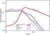 |
Fig. 2 Normal optical depth for the same ACE runs and time instants as in Fig. 1. |
| In the text | |
|
Fig. 3 Lifetimes of dust grains and parent bodies for the same ACE runs and time instants as in Fig. 1. Particles below the 3.8 Gyr line are in a collisional equilibrium after the LHB. A steep rise in the lifetime at s ~ 300 m corresponds to the strength-gravity transition of the critical disruption energy. |
| In the text | |
|
Fig. 4 Capture probability of a single particle with given β and e at the location of the 3:2 resonance with Neptune. |
| In the text | |
|
Fig. 5 Capture probability of a β particle released by a parent body for the 3:2 resonance with Neptune. ep = 0.6 represents the population of scattered objects. Note that all particles above the horizontal lines have initial eccentricites of e > 1 and will be removed from the system (Eq. (7)). |
| In the text | |
|
Fig. 6 Temperatures of the dirty-ice particles for different distances. The solid lines correspond to 100 K, 75 K and 50 K. Sublimation occurs at Tsubl = 100 K. Sublimation distance increases with decreasing size because the emission efficiency of small grains is lower, which makes them hotter. |
| In the text | |
|
Fig. 7 Simulated particle flux compared with in-situ measurements by New Horizons and Voyager 1 and 2. The solid black line takes into account planets and sublimation and represents our best fit to the data taken from Poppe et al. (2010), Han et al. (2011) and Gurnett et al. (1997). The dotted and dashed lines show the dust flux for the unperturbed EKB and after planetary scattering without sublimation, respectively. |
| In the text | |
|
Fig. 8 Spectral energy distribution of the EKB including planets and sublimation (solid black line), without sublimation (dashed red line), and for an unperturbed EKB (dottted blue line). All curves are based on the same run (“f”) and the same time instant as in Fig. 7. |
| In the text | |
Current usage metrics show cumulative count of Article Views (full-text article views including HTML views, PDF and ePub downloads, according to the available data) and Abstracts Views on Vision4Press platform.
Data correspond to usage on the plateform after 2015. The current usage metrics is available 48-96 hours after online publication and is updated daily on week days.
Initial download of the metrics may take a while.