| Issue |
A&A
Volume 540, April 2012
|
|
|---|---|---|
| Article Number | A70 | |
| Number of page(s) | 10 | |
| Section | Cosmology (including clusters of galaxies) | |
| DOI | https://doi.org/10.1051/0004-6361/201118543 | |
| Published online | 28 March 2012 | |
Analytical properties of Einasto dark matter haloes
1
Escuela de Física, Universidad de Costa Rica,
11501
San Pedro,
Costa Rica
e-mail: This email address is being protected from spambots. You need JavaScript enabled to view it.
2
Sterrenkundig Observatorium, Universiteit Gent,
Krijgslaan 281-S9,
9000
Gent,
Belgium
e-mail: This email address is being protected from spambots. You need JavaScript enabled to view it.
Received:
29
November
2011
Accepted:
19
January
2012
Abstract
Recent high-resolution N-body CDM simulations indicate that nonsingular three-parameter models such as the Einasto profile perform better than the singular two-parameter models, e.g. the Navarro, Frenk and White, in fitting a wide range of dark matter haloes. While many of the basic properties of the Einasto profile have been discussed in previous studies, a number of analytical properties are still not investigated. In particular, a general analytical formula for the surface density, an important quantity that defines the lensing properties of a dark matter halo, is still lacking to date. To this aim, we used a Mellin integral transform formalism to derive a closed expression for the Einasto surface density and related properties in terms of the Fox H and Meijer G functions, which can be written as series expansions. This enables arbitrary-precision calculations of the surface density and the lensing properties of realistic dark matter halo models. Furthermore, we compared the Sérsic and Einasto surface mass densities and found differences between them, which implies that the lensing properties for both profiles differ.
Key words: gravitational lensing: weak / galaxies: clusters: general / dark matter / methods: analytical / galaxies: halos / gravitational lensing: strong
© ESO, 2012
1. Introduction
The Λ cold dark matter (CDM) model, with (Ωm, ΩΛ) = (0.3, 0.7), has become the standard theory of cosmological structure formation. ΛCDM seems to agree with the observations on cluster-sized scales (Primack 2003); however, on galaxy/sub-galaxy scales there appears to be a discrepancy between observations and numerical simulations. High-resolution observations of rotation curves, in particular of low surface brightness (LSB) and dark matter dominated dwarf galaxies (de Blok et al. 2001; van den Bosch & Swaters 2001; Swaters et al. 2003; Weldrake et al. 2003; Donato et al. 2004; Gentile et al. 2005; Simon et al. 2005; Gentile et al. 2007; Banerjee et al. 2010) favour density profiles with a flat central core (e.g. Burkert 1995; Salucci & Burkert 2000; Gentile et al. 2004; Li & Chen 2009). In contrast, N-body (dark matter only) CDM simulations predict galactic density profiles that are too high in the centre (e.g. Navarro et al. 1996, 1997, NFW; Moore et al. 1999). This discrepancy is called the cusp-core problem; a complete review can be found in de Blok (2010).
Gravitational lensing is one of the most powerful tools in observational cosmology for probing the matter distribution of galaxies and clusters in the strong regime (Kochanek et al. 1989; Wambsganss & Paczynski 1994; Bartelmann 1996; Chae et al. 1998; Kochanek et al. 2000; Keeton & Madau 2001; Sand et al. 2002; Keeton 2002, 2003; Keeton & Zabludoff 2004; Limousin et al. 2008; Anguita et al. 2009; Zitrin et al. 2011a,b) and the weak regime (Kaiser & Squires 1993; Mellier 1999; Bartelmann & Schneider 2001; Hoekstra et al. 2004; Clowe et al. 2006; Mahdavi et al. 2007; Jee et al. 2009; Huang et al. 2011). Comparing these observations to theoretical models provides key information to help resolve the cusp-core problem. Evidently, one must use the most accurate density profile to obtain the best fit to observational data from strong- and weak-lensing studies.
Recently, N-body CDM simulations (Navarro
et al. 2004; Merritt et al. 2006; Gao et al. 2008; Hayashi
& White 2008; Stadel et al. 2009;
Navarro et al. 2010) have found that certain
three-parameter profiles provide an excellent fit to a wide range of dark matter haloes. One
of these is the Einasto (1965) profile, a
three-dimensional version of the two-dimensional Sérsic
(1968) profile used to describe the surface brightness of early-type galaxies and
the bulges of spiral galaxies (e.g. Davies et al.
1988; Caon et al. 1993; D’Onofrio et al. 1994; Cellone et al. 1994; Andredakis et al. 1995;
Prugniel & Simien 1997; Möllenhoff & Heidt 2001; Graham & Guzmán 2003; Graham
et al. 2006; Gadotti 2009). The Sérsic
profile can be written as: ![Mathematical equation: \begin{equation} \Sigma_{\text{S}}\left(R\right) = \Upsilon I_{{\text{e}}}\exp\left\{ -b_{\rm m}\left[\left(\frac{R}{R_{{\text{e}}}}\right)^{1/m}- 1\right]\,\right\} ,\label{eq:Sersic-surface-mass-density} \end{equation}](/articles/aa/full_html/2012/04/aa18543-11/aa18543-11-eq6.png) (1)where R is
the distance in the sky plane, m the Sérsic index, Υ is the mass-to-light
ratio, Ie is the luminosity density at the effective radius
Re, and bm is a dimensionless
function of m that can be determined from the condition that the luminosity
inside Re equals half of the total luminosity. Numerical
solutions for bm are given by Ciotti (1991), Moriondo et al. (1998),
Prugniel & Simien (1997) and an asymptotic
expansion
(1)where R is
the distance in the sky plane, m the Sérsic index, Υ is the mass-to-light
ratio, Ie is the luminosity density at the effective radius
Re, and bm is a dimensionless
function of m that can be determined from the condition that the luminosity
inside Re equals half of the total luminosity. Numerical
solutions for bm are given by Ciotti (1991), Moriondo et al. (1998),
Prugniel & Simien (1997) and an asymptotic
expansion  using analytical methods was obtained by Ciotti &
Bertin (1999).
using analytical methods was obtained by Ciotti &
Bertin (1999).
The Einasto profile (model) is characterised by a power-law logarithmic slope,
 (2)with n,
which we call the Einasto index, a positive number defining the steepness of the power law.
Integrating leads to the general density profile
(2)with n,
which we call the Einasto index, a positive number defining the steepness of the power law.
Integrating leads to the general density profile
![Mathematical equation: \begin{equation} \rho(r)=\rho_{\text{s}}\exp\left\{ -d_{n}\left[\left(\frac{r}{{r_{{\text{s}}}}}\right)^{1/n}-1\right]\,\right\}, \end{equation}](/articles/aa/full_html/2012/04/aa18543-11/aa18543-11-eq16.png) (3)where
rs represents the radius of the sphere that contains half of
the total mass, ρs is the mass density at
r = rs, and
dn is a numerical constant that ensures
that rs is indeed the half-mass radius. In the context of dark
matter haloes, the density can also be expressed as
(3)where
rs represents the radius of the sphere that contains half of
the total mass, ρs is the mass density at
r = rs, and
dn is a numerical constant that ensures
that rs is indeed the half-mass radius. In the context of dark
matter haloes, the density can also be expressed as ![Mathematical equation: \begin{equation} \rho\left(r\right) = \rho_{-2}\,\exp\left\{ -2n\left[\left(\frac{r}{r_{-2}}\right)^{1/n}-1\right]\,\right\}, \label{eq:einasto_halo_vers} \end{equation}](/articles/aa/full_html/2012/04/aa18543-11/aa18543-11-eq21.png) (4)where
ρ-2 and r-2 are the density and
radius at which
(4)where
ρ-2 and r-2 are the density and
radius at which  .
In the remainder of this paper, we will use yet another, equivalent version,
.
In the remainder of this paper, we will use yet another, equivalent version, ![Mathematical equation: \begin{equation} \rho(r)=\rho_{0}\exp\left[-\left(\frac{r}{h}\right)^{1/n}\right],\label{eq:einasto_gen_vers} \end{equation}](/articles/aa/full_html/2012/04/aa18543-11/aa18543-11-eq25.png) (5)where we introduced the
central density
(5)where we introduced the
central density  (6)and the scale length
 (7)If a model is to describe
real galactic systems, several conditions must be imposed on the model description
functions, as discussed by Einasto (1969a). When a
model is constructed, an initial descriptive function is chosen; the most practical choice
is the density profile, because the main descriptive functions (cumulative mass profile,
gravitational potential, surface mass density) are integrals of the density profile.
Furthermore, a physical model has to satisfy several conditions: i) the density profile must
be non-negative and finite; ii) the density must be a smoothly decreasing function that
approaches zero at large radii; iii) some moments of the mass function must be finite, in
particular moments that define the central gravitational potential, the total mass, and the
effective radius of the system; and iv) the descriptive functions must not have jump
discontinuities. Einasto (1969a) presented several
families of valid descriptive functions, among which the so-called Einasto profile is a
special case that agrees best with observations.
(7)If a model is to describe
real galactic systems, several conditions must be imposed on the model description
functions, as discussed by Einasto (1969a). When a
model is constructed, an initial descriptive function is chosen; the most practical choice
is the density profile, because the main descriptive functions (cumulative mass profile,
gravitational potential, surface mass density) are integrals of the density profile.
Furthermore, a physical model has to satisfy several conditions: i) the density profile must
be non-negative and finite; ii) the density must be a smoothly decreasing function that
approaches zero at large radii; iii) some moments of the mass function must be finite, in
particular moments that define the central gravitational potential, the total mass, and the
effective radius of the system; and iv) the descriptive functions must not have jump
discontinuities. Einasto (1969a) presented several
families of valid descriptive functions, among which the so-called Einasto profile is a
special case that agrees best with observations.
The Einasto profile was used by Einasto (1969b) to obtain a model of M31. Later, this model was applied by Einasto (1974) to several nearby galaxies, including M32, M87, Fornax and Sculptor dwarfs, and also M31 and the Milky Way. These models were multi-component ones, and each component has its own parameter set {ρ0, h, n} representing certain physically homogeneous stellar populations.
Navarro et al. (2004) found that for haloes with masses from dwarfs to clusters, 4.54 ≲ n ≲ 8.33 with an average value of n = 5.88. Hayashi & White (2008) and Gao et al. (2008) found that n tends to decrease with mass and redshift, with n ~ 5.88 for galaxy-sized and n ~ 4.35 for cluster-sized haloes in the Millennium Run (MR) (Springel et al. 2005). Navarro et al. (2010) obtained similar results for galaxy-sized haloes in the Aquarius simulation (Springel et al. 2008). Also, Gao et al. (2008) showed that n ~ 3.33 for the most massive haloes of MR. Chemin et al. (2011) modelled the rotation curves of a spiral galaxies subsample from THINGS (The HI Nearby Galaxy Survey, de Blok et al. 2008), using the Einasto profile, and found that n tends to have lower values by a factor of two or more compared to those predicted by N-body simulations. Dhar & Williams (2012) fitted the surface brightness profiles of a large sample of elliptical galaxies in the Virgo cluster, using a multi-component Einasto profile consisting of two or three components for each galaxy with different n for each individual component. For the central component, they found values of n ≲ 1 for the most massive and shallow-cusp galaxies and n < 2 for steep-cusp galaxies, while 5 ≲ n ≲ 8 for the outer component of massive galaxies. These values for the outer component are consistent with the results from N-body simulations for Einasto dark matter haloes, and the authors argued that Einasto components with an n in this range could be dark matter dominated.
In the light of its increasing popularity to describe the density of simulated dark matter haloes, a detailed investigation of the properties of the Einasto model is of paramount importance. Some aspects of the Einasto model have been presented by several authors (Mamon & Łokas 2005; Cardone et al. 2005; Merritt et al. 2006; Dhar & Williams 2010). The most complete study of the properties of the Einasto model is the work by Cardone et al. (2005), who provided a set of analytical expressions for quantities such as the mass profile and gravitational potential and discussed the dynamical structure for both isotropic and anisotropic cases. Nevertheless, the Einasto model has not been studied analytically as extensively as the Sérsic models, and several properties still have to be further investigated in more detail. One area where progress is still to be made is on the value of the dimensionless parameter dn.
The most important lacuna, however, concerns the surface density on the plane of the sky, an important quantity that defines the lensing properties of a dark matter halo. The surface mass density has an importance in theoretical predictions and observations. On the observational side, based mostly on the mass decomposition of rotation curves using cored haloes, various studies (Kormendy & Freeman 2004; Spano et al. 2008; Donato et al. 2009; Gentile et al. 2009) have shown that the product of the central density ρ0 and the core radius r0 is consistent with a universal value, independent of galaxy mass. The product ρ0r0 is directly proportional to the average surface density within r0, and to the gravitational acceleration of dark matter at r0. In view of a detailed comparison of these results with the outcome of the most recent dark matter simulations, it is therefore important to study the analytical properties of the surface density distribution of Einasto haloes. Recent works studying theoretical and observational aspects of dark matter surface densities include Boyarsky et al. (2010), Walker et al. (2010), Napolitano et al. (2010), and Cardone et al. (2011): efforts are being made to confirm or call into question the universality of the dark matter surface density within one dark halo scale length.
Cardone et al. (2005) showed that the surface density of the Einasto model cannot be expressed in terms of elementary functions and discussed the general properties using numerical integration. Dhar & Williams (2010) presented an analytical approximation for the Einasto surface brightness profile and demonstrated that this surface density profile is not Sérsic-like. A general analytical formula, which would enable an arbitrary-precision calculation and an analytical study of the asymptotic behaviour, is still lacking to date.
The most recent studies in strong and weak lensing (e.g. Donnarumma et al. 2011; Sereno & Umetsu 2011; Morandi et al. 2011; Umetsu et al. 2011; Oguri et al. 2012) use the NFW profile or its generalization (Zhao 1996; Jing & Suto 2000) to model the dark matter halo instead of the Einasto profile. One of the factors that limits its adoption is the absence of analytical formulas for its lensing properties. Therefore, its application in lensing studies is not as wide as for other profiles. A complete general set of analytical formulas for the lensing properties of the Einasto profile would help to increase its use in lensing studies.
In this paper, we extend the analytical study of the Einasto model using some of the techniques also employed in the extensive literature on the analytical properties of the Sérsic model (e.g. Ciotti 1991; Ciotti & Lanzoni 1997; Ciotti & Bertin 1999; Trujillo et al. 2001; Mazure & Capelato 2002; Cardone 2004; Graham & Driver 2005; Elíasdóttir & Möller 2007; Baes & Gentile 2011; Baes & van Hese 2011). In Sect. 2, we discuss an analytical expansion for the dimensionless parameter dn. In Sect. 3, we derive an analytical expression for the Einasto surface mass density in terms of the Fox H function, using the Mellin transform-method. We then use the result for the projected surface mass density to calculate the cumulative surface mass, lens equation, deflection angle, deflection potential, magnification, shear and the critical curves for a spherically symmetric lens described by the Einasto profile in terms of this function. We also calculate explicit series expansions for the surface mass density and all the lensing properties. In Sect. 4, we derive some special cases for the lensing properties for integer and half-integer values of n in terms of the Meijer G function. Furthermore, we compare the Einasto and Sérsic surface mass densities for the same values of their respective indices. Finally, in Sect. 5 we discuss the asymptotic behaviour of the surface mass density and cumulative surface mass at small and large radii. We present our conclusions in Sect. 6.
2. Spatial properties
The total mass of an Einasto model with a mass density profile given by (5), is  (8)If we use this formula to
replace the central density ρ0 by the total mass
M as a parameter in the definition of the Einasto models, we obtain
(8)If we use this formula to
replace the central density ρ0 by the total mass
M as a parameter in the definition of the Einasto models, we obtain
 (9)where we have introduced
the reduced radius
(9)where we have introduced
the reduced radius  (10)At small radii, the
density profile behaves as
(10)At small radii, the
density profile behaves as  (11)The cumulative mass profile
M(r) of a spherical mass distribution is found through
the equation
(11)The cumulative mass profile
M(r) of a spherical mass distribution is found through
the equation 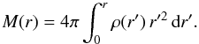 (12)For the Einasto
model, we find
(12)For the Einasto
model, we find ![Mathematical equation: \begin{equation} M(r)=M\left[1-\frac{\Gamma(3n,s^{1/n})}{\Gamma(3n)}\right], \end{equation}](/articles/aa/full_html/2012/04/aa18543-11/aa18543-11-eq47.png) (13)where
Γ(α,x) is the incomplete gamma function,
(13)where
Γ(α,x) is the incomplete gamma function,
 (14)Given that this is
the radius of the sphere that encloses half of the total mass, we find that
dn is the solution of the equation
(14)Given that this is
the radius of the sphere that encloses half of the total mass, we find that
dn is the solution of the equation
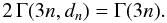 (15)This equation cannot be
solved in a closed form; one option is to solve it numerically or use interpolation
formulae. For example, Merritt et al. (2006), quoting
G. A. Mamon (priv. comm.), propose
(15)This equation cannot be
solved in a closed form; one option is to solve it numerically or use interpolation
formulae. For example, Merritt et al. (2006), quoting
G. A. Mamon (priv. comm.), propose 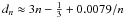 , but do
not mention the origin of this approximation or quote its accuracy. An elegant way to
determine an approximation for dn builds on the
work by Ciotti & Bertin (1999), who used an
asymptotic expansion method to solve the general relation
Γ(α,x) = Γ(α)/2. If we apply the
resulting expansion to our problem, we obtain for the parameter
dn from the Einasto model
, but do
not mention the origin of this approximation or quote its accuracy. An elegant way to
determine an approximation for dn builds on the
work by Ciotti & Bertin (1999), who used an
asymptotic expansion method to solve the general relation
Γ(α,x) = Γ(α)/2. If we apply the
resulting expansion to our problem, we obtain for the parameter
dn from the Einasto model 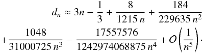 (16)The
gravitational potential of a spherically symmetric mass distribution
ρ(r) can be found through the formula
(16)The
gravitational potential of a spherically symmetric mass distribution
ρ(r) can be found through the formula
![Mathematical equation: \begin{equation} \Psi(r) = 4\pi G\left[\frac{1}{r}\int_{0}^{r}\rho(r')\, r'^{2}\,{\text{d}}r'+\int_{r}^{\infty}\rho(r')\, r'\,{\text{d}}r'\right], \end{equation}](/articles/aa/full_html/2012/04/aa18543-11/aa18543-11-eq55.png) (17)or equivalently
(17)or equivalently
 (18)For the Einasto model, we
find
(18)For the Einasto model, we
find ![Mathematical equation: \begin{equation} \Psi(r) = \frac{GM}{h}\, s^{-1}\left[1-\frac{\Gamma(3n,s^{1/n})}{\Gamma(3n)}+\frac{s\,\Gamma(2n,s^{1/n})}{\Gamma(3n)}\right]\cdot \end{equation}](/articles/aa/full_html/2012/04/aa18543-11/aa18543-11-eq57.png) (19)The Einasto model has a
finite potential well, given by
(19)The Einasto model has a
finite potential well, given by  (20)At small radii, the
potential decreases parabolically
(20)At small radii, the
potential decreases parabolically ![Mathematical equation: \begin{equation} \Psi(r) \sim \frac{GM}{h}\,\left[\frac{\Gamma(2n)}{\Gamma(3n)}-\frac{s^{2}}{6n\,\Gamma(3n)}+\ldots\right], \end{equation}](/articles/aa/full_html/2012/04/aa18543-11/aa18543-11-eq59.png) (21)which is not
surprising, given the finite density core of the Einasto density profile. At large radii, we
obtain a Keplerian fall-off,
(21)which is not
surprising, given the finite density core of the Einasto density profile. At large radii, we
obtain a Keplerian fall-off,  (22)which is also
expected for a model with a finite total mass.
(22)which is also
expected for a model with a finite total mass.
3. Lensing properties
3.1. Surface mass density and cumulative surface mass density
The surface mass density of a spherically symmetric lens is given by integrating along
the line of sight of the 3D density profile  (23)where
ξ is the radius measured from the centre of the lens and
(23)where
ξ is the radius measured from the centre of the lens and
 .
This expression can also be written as an Abel transform (Binney & Tremaine 1987)
.
This expression can also be written as an Abel transform (Binney & Tremaine 1987)  (24)Inserting Eq. (5) into the above expression, we obtain
 (25)where we have introduced
the quantities
x = ξ/h and
s = r/h.
(25)where we have introduced
the quantities
x = ξ/h and
s = r/h.
As discussed by Cardone et al. (2005) and Dhar & Williams (2010), the integral (25) cannot be expressed in terms of elementary
or even the most regular functions for all the values of n. Only the
central surface mass density can be evaluated analytically as  (26)This situation is
very similar to the deprojection of the Sérsic surface brightness profile (1). Indeed, the deprojection formula leads to
an integral that is an inverse Abel transform, and also in this case it was long thought
that no further analytical progress was possible. However, Mazure & Capelato (2002) used the computer package Mathematica to
demonstrate that it is possible to write the Sérsic luminosity density in terms of the
Meijer G function for all integer Sérsic indices m.
Baes & Gentile (2011) and Baes & van Hese (2011) took this analysis one
step further and showed that the deprojection of the Sérsic surface brightness profile for
general values of m can be solved elegantly using Mellin integral
transforms and gives rise to a Mellin-Barnes integral. The result is that the Sérsic
luminosity density can be written compactly in terms of a Fox H function,
which reduces to a Meijer G function for all rational values of
m.
(26)This situation is
very similar to the deprojection of the Sérsic surface brightness profile (1). Indeed, the deprojection formula leads to
an integral that is an inverse Abel transform, and also in this case it was long thought
that no further analytical progress was possible. However, Mazure & Capelato (2002) used the computer package Mathematica to
demonstrate that it is possible to write the Sérsic luminosity density in terms of the
Meijer G function for all integer Sérsic indices m.
Baes & Gentile (2011) and Baes & van Hese (2011) took this analysis one
step further and showed that the deprojection of the Sérsic surface brightness profile for
general values of m can be solved elegantly using Mellin integral
transforms and gives rise to a Mellin-Barnes integral. The result is that the Sérsic
luminosity density can be written compactly in terms of a Fox H function,
which reduces to a Meijer G function for all rational values of
m.
The obvious similarity between these two cases invites us to apply the same Mellin
transform technique (Marichev 1982; Adamchick 1996; Fikioris
2007) to the integral (25). The
basic idea behind this technique is that any definite integral  (27)can be written as
 (28)This expression is
exactly a Mellin convolution of two functions f1 and
f2. Now we can apply the Mellin convolution theorem, which
states that the Mellin transform of a Mellin convolution is equal to the products of the
Mellin transforms of the original functions. As a result, the definite integral (27) can be written as the inverse Mellin
transform of the product of the Mellin transforms of f1 and
f2. The Mellin transform and its inverse are defined as
(28)This expression is
exactly a Mellin convolution of two functions f1 and
f2. Now we can apply the Mellin convolution theorem, which
states that the Mellin transform of a Mellin convolution is equal to the products of the
Mellin transforms of the original functions. As a result, the definite integral (27) can be written as the inverse Mellin
transform of the product of the Mellin transforms of f1 and
f2. The Mellin transform and its inverse are defined as
 with
ℒ a line integral over a vertical line in the complex plane. This implies that
with
ℒ a line integral over a vertical line in the complex plane. This implies that
 (31)It now turns out
that the integral (31) is a Mellin-Barnes
integral for large classes of the functions f1 and
f2, and that this integral can be evaluated as a Fox
H function or a Meijer G function in many cases.
(31)It now turns out
that the integral (31) is a Mellin-Barnes
integral for large classes of the functions f1 and
f2, and that this integral can be evaluated as a Fox
H function or a Meijer G function in many cases.
We can immediately apply this formalism to the integral (25), with z = 1 and
 (32)and
 (33)The
Mellin transforms of these functions are readily calculated
(33)The
Mellin transforms of these functions are readily calculated
![Mathematical equation: \begin{eqnarray} {\mathfrak{M}}_{f_{1}}(u)=2\,\rho_{0}\, h\, n\,\Gamma\,[n(2+u)],\\ {\mathfrak{M}}_{f_{2}}(u)=\frac{\sqrt{\pi}\,\Gamma\left(\frac{1+u}{2}\right)}{\Gamma\left(\frac{u}{2}\right)}\,\frac{1}{u\, x^{1+u}}\cdot \end{eqnarray}](/articles/aa/full_html/2012/04/aa18543-11/aa18543-11-eq79.png) Combining
these results, we obtain
Combining
these results, we obtain ![Mathematical equation: \begin{eqnarray} \Sigma(x)&& = 2n\,\sqrt{\pi}\,\rho_{0}\, h\, x\,\nonumber \\ \label{eq:Sigma-contour} &&\times\,\frac{1}{2\pi \rm i}\int_{\mathcal{L}}\frac{\Gamma\left(2ny\right)\Gamma\left(-\frac{1}{2}+y\right)}{\Gamma\left (y\right)}\left[\, x^{2}\right]^{-y}{\text{d}}y. \end{eqnarray}](/articles/aa/full_html/2012/04/aa18543-11/aa18543-11-eq80.png) (36)This
Mellin-Barnes integral may be recognized as a Fox H function, which is
generally defined as the inverse Mellin transform of a product of gamma-functions,
(36)This
Mellin-Barnes integral may be recognized as a Fox H function, which is
generally defined as the inverse Mellin transform of a product of gamma-functions,
![Mathematical equation: \begin{eqnarray} H_{p,q}^{m,n}\left[\left.\begin{matrix}({\boldsymbol{a}},{\boldsymbol{A}})\notag\\ ({\boldsymbol{b}},{\boldsymbol{B}}) \end{matrix}\,\right|\, z\right]&&=\notag\\ label{eq:defH} &&\frac{1}{2\pi \rm i}\int_{{\cal L}}\frac{\prod_{j=1}^{m}\Gamma(b_{j}+B_{j}s)\prod_{j=1}^{n}\Gamma(1-a_{j}-A_{j}s)}{\prod_{j=m+1}^{q}\Gamma(1-b_{j}-B_{j}s)\prod_{j=n+1}^{p}\Gamma(a_{j}+A_{j}s)}\, z^{-s}\,{\text{d}}s.\ \end{eqnarray}](/articles/aa/full_html/2012/04/aa18543-11/aa18543-11-eq81.png) (37)Using
this definition, we can write the surface density of the Einasto model in the following
compact form,
(37)Using
this definition, we can write the surface density of the Einasto model in the following
compact form, ![Mathematical equation: \begin{equation} \Sigma\left(x\right)=2n\,\sqrt{\pi}\,\rho_{0}\, h\, x\, H_{1,2}^{2,0}\left[\begin{array}{c} (0,\,1)\\ (0,\,2n),(-\frac{1}{2},\,1) \end{array}\biggr|\, x^{2}\right].\label{eq:Sigma-Fox} \end{equation}](/articles/aa/full_html/2012/04/aa18543-11/aa18543-11-eq82.png) (38)The Fox
H function is a general analytical function that is becoming more and
more used both in mathematics and applied sciences; in fact, it is scheduled for inclusion
in the Mathematica numerical library. While not the most mainstream special function, the
Fox H is an extremely flexible function that contains very broad classes
of elementary and special functions as particular cases. It is indeed a very powerful tool
for analytical work. It has many general properties that allow one to manipulate
expressions to equivalent forms, reduce the order for certain values of the parameters,
etc. For details on its many useful properties, we refer the interested reader to Mathai (1978), Kilbas
& Saigo (2004), or Mathai et al.
(2009) and the references therein.
(38)The Fox
H function is a general analytical function that is becoming more and
more used both in mathematics and applied sciences; in fact, it is scheduled for inclusion
in the Mathematica numerical library. While not the most mainstream special function, the
Fox H is an extremely flexible function that contains very broad classes
of elementary and special functions as particular cases. It is indeed a very powerful tool
for analytical work. It has many general properties that allow one to manipulate
expressions to equivalent forms, reduce the order for certain values of the parameters,
etc. For details on its many useful properties, we refer the interested reader to Mathai (1978), Kilbas
& Saigo (2004), or Mathai et al.
(2009) and the references therein.
As an illustration of the power of the Fox H function as an analytical
tool, and as a sanity check on the formula, we can calculate the total mass of the Einasto
model by integrating the surface mass density over the plane of the sky,
![Mathematical equation: \begin{eqnarray} M=2\pi\int_{0}^{\infty}\Sigma(\xi)\,\xi\,{\text{d}}\xi&=&2n\,\pi^{3/2}\,\rho_{0}\, h^{3}\,\notag\\ &&\times\ \int_{0}^{\infty}H_{1,2}^{2,0}\left[\begin{array}{c} (0,\,1)\\ (0,\,2n),(-\frac{1}{2},\,1) \end{array}\biggr|\, t\right]\, t^{1/2}{\text{d}}t.\quad\quad\quad \end{eqnarray}](/articles/aa/full_html/2012/04/aa18543-11/aa18543-11-eq83.png) (39)This
integral can be calculated by setting
(39)This
integral can be calculated by setting  and
a = 1 in Eq. (2.8) in Mathai et al.
(2009). We immediately find
and
a = 1 in Eq. (2.8) in Mathai et al.
(2009). We immediately find
 (40)in agreement with
Eq. (8).
(40)in agreement with
Eq. (8).
An important quantity for gravitational lensing studies is the cumulative surface mass
density, i.e. the total mass contained in a infinite cylinder with radius
ξ,  (41)We find
![Mathematical equation: \begin{eqnarray} M(x)&=&2n\,\pi^{3/2}\,\rho_{0}\, h^{3}\, x^{3}\,\nonumber\\ &&\label{eq:M-Fox}\times\, H_{2,3}^{2,1}\left[ \begin{array}{c} (-\frac{1}{2},\,1),(0,\,1)\\ (0,\,2n),(-\frac{1}{2},\,1),(-\frac{3}{2},\,1) \end{array}\biggr|\, x^{2}\right]. \end{eqnarray}](/articles/aa/full_html/2012/04/aa18543-11/aa18543-11-eq88.png) (42)As
another demonstration of the usefulness of the Fox H function, we can
apply the residue theorem to the contour integral (37), and obtain
explicit series expansions. The general procedure can be found in Kilbas & Saigo (1999), and a specific application to the
deprojected Sérsic model is given in Baes & van
Hese (2011). The analysis for the projected Einasto profile is completely
analogous: again, the form of the series expansion depends on the multiplicity of the
poles of the gamma functions
Γ(bj + Bjs).
For both Σ(x) and M(x), the poles of
these gamma functions are
−k1/2n and
1/2 − k2, with
k1 and k2 any natural number. We
encounter two cases.
(42)As
another demonstration of the usefulness of the Fox H function, we can
apply the residue theorem to the contour integral (37), and obtain
explicit series expansions. The general procedure can be found in Kilbas & Saigo (1999), and a specific application to the
deprojected Sérsic model is given in Baes & van
Hese (2011). The analysis for the projected Einasto profile is completely
analogous: again, the form of the series expansion depends on the multiplicity of the
poles of the gamma functions
Γ(bj + Bjs).
For both Σ(x) and M(x), the poles of
these gamma functions are
−k1/2n and
1/2 − k2, with
k1 and k2 any natural number. We
encounter two cases.
Case 1: if n is either non-rational or a rational number
p/q with an even denominator (and
p,q coprime), all poles are simple and the expansion is a power series,
![Mathematical equation: \begin{eqnarray} \Sigma(x)=2n\sqrt{\pi}\,\rho_{0}\, h\,\left[\sum_{k=1}^{\infty}\frac{\Gamma\left(-\tfrac{1}{2}-\tfrac{k}{2n}\right)}{\Gamma\left(-\tfrac{k}{2n}\right)}\,\frac{(-1)^{k}}{k!}\,\frac{x^{k/n+1}}{2n}\right.\notag\\ \label{sigma-gen-series} \left.+\sum_{k=0}^{\infty}\frac{\Gamma(n-2nk)}{\Gamma\left(\tfrac{1}{2}-k\right)}\,\frac{(-1)^{k}}{k!}\, x^{2k}\right], \end{eqnarray}](/articles/aa/full_html/2012/04/aa18543-11/aa18543-11-eq99.png) (43)and
(43)and
![Mathematical equation: \begin{eqnarray} M(x)=2n\,\pi^{3/2}\,\rho_{0}\, h^{3}\,\left[-\sum_{k=1}^{\infty}\frac{\Gamma\left(-\tfrac{3}{2}-\tfrac{k}{2n}\right)}{\Gamma\left(-\tfrac{k}{2n}\right)}\,\frac{(-1)^{k}}{k!}\,\frac{x^{k/n+3}}{2n}\right.\notag\\ \label{mass-gen-series} \left.+\sum_{k=0}^{\infty}\frac{\Gamma(n-2nk)}{\Gamma\left(\tfrac{1}{2}-k\right)}\,\frac{(-1)^{k}}{(k+1)!}\, x^{2k+2}\right]. \end{eqnarray}](/articles/aa/full_html/2012/04/aa18543-11/aa18543-11-eq100.png) (44)Case
2: if n is integer or a rational number
p/q with an odd denominator, some
poles are of second order, and the expansion is a logarithmic-power series. If we define
(44)Case
2: if n is integer or a rational number
p/q with an odd denominator, some
poles are of second order, and the expansion is a logarithmic-power series. If we define
 ,
then we obtain after some algebra
,
then we obtain after some algebra
![Mathematical equation: \begin{eqnarray} \Sigma(x)&=&2n\sqrt{\pi}\,\rho_{0}\, h\,\left[\;\sum_{\substack{k=1\\ k\,{\text{mod}}\, p\ne0 } }^{\infty}\hspace{-1.5ex}\frac{\Gamma\left(-\tfrac{1}{2}-\tfrac{k}{2n}\right)}{\Gamma\left(-\tfrac{k}{2n}\right)}\,\frac{(-1)^{k}}{k!}\,\frac{x^{k/n+1}}{2n}\right.\nonumber\\ &&\left.\ +\ \frac{\Gamma(n)}{\sqrt{\pi}}\ +\ \hspace{-3ex}\sum_{\substack{k=1\\ (k+k_{0})\,{\text{mod}}\, q\ne0 } }^{\infty}\hspace{-3ex}\frac{\Gamma(n-2nk)}{\Gamma\left(\tfrac{1}{2}-k\right)}\,\frac{(-1)^{k}}{k!}\, x^{2k}\right]\nonumber\\ && + 2\,\rho_{0}\, h\,\hspace{-3ex}\sum_{\substack{k=0\\ (k+k_{0})\,{\text{mod}}\, q=0 } }^{\infty}\hspace{-3ex}\frac{(-1)^{p}\,(2k)!}{(2nk-n)!\, k!\, k!}\,\left(\frac{x}{2}\right)^{2k}\ \times\left[-\ln\left(\frac{x}{2}\right)\right.\nonumber\\ \label{sigma-rat-series}&&\left.-\frac{1}{2k}+\psi(k+1)+n\,\psi(2nk-n)-\psi(2k-1)\right], \end{eqnarray}](/articles/aa/full_html/2012/04/aa18543-11/aa18543-11-eq103.png) (45)and
(45)and
![Mathematical equation: \begin{eqnarray} && M(x)=2n\,\pi^{3/2}\,\rho_{0}\, h^{3}\, x^{2}\,\left[\ \ -\hspace{-1.5ex}\sum_{\substack{k=1\\ k\,{\text{mod}}\, p\ne0 } }^{\infty}\hspace{-1ex}\frac{\Gamma\left(-\tfrac{3}{2}-\tfrac{k}{2n}\right)}{\Gamma\left(-\tfrac{k}{2n}\right)}\,\frac{(-1)^{k}}{k!}\,\frac{x^{k/n+1}}{2n}\right.\nonumber\\ &&\quad\,\left.+\ \frac{\Gamma(n)}{\sqrt{\pi}}\ +\ \hspace{-3ex}\sum_{\substack{k=1\\ (k+k_{0})\,{\text{mod}}\, q\ne0 } }^{\infty}\hspace{-3ex}\frac{\Gamma(n-2nk)}{\Gamma\left(\tfrac{1}{2}-k\right)}\,\frac{(-1)^{k}}{(k+1)!}\, x^{2k}\right]\nonumber\\ &&\quad\, + 2\pi\,\rho_{0}\, h^{3}\, x^{2}\,\hspace{-3ex}\sum_{\substack{k=0\\ (k+k_{0})\,{\text{mod}}\, q=0 } }^{\infty}\hspace{-3ex}\frac{(-1)^{p}\,(2k)!}{(2nk-n)!\, k!\,(k+1)!}\left(\frac{x}{2}\right)^{2k}\times\ \left[-\ln\left(\frac{x}{2}\right)\right.\nonumber\\ \label{mass-rat-series}&&\quad\,\left.-\frac{1}{2k}-\frac{1}{2k+2}+\psi(k+2)+n\,\psi(2nk-n)-\psi(2k-1)\right], \end{eqnarray}](/articles/aa/full_html/2012/04/aa18543-11/aa18543-11-eq104.png) (46)
with
ψ(k) the digamma function.
(46)
with
ψ(k) the digamma function.
3.2. Lens equation and deflection angle
In the thin lens approximation, the lens equation for axially symmetric lens is
 (47)where the
quantities η and ξ are the physical positions of the
source in the source plane and an image in the image plane, respectively,
(47)where the
quantities η and ξ are the physical positions of the
source in the source plane and an image in the image plane, respectively,
 is the deflection angle, and DL,
DS and DLS are the angular
distances from observer to lens, from observer to source, and from lens to source,
respectively.
is the deflection angle, and DL,
DS and DLS are the angular
distances from observer to lens, from observer to source, and from lens to source,
respectively.
With the dimensionless positions
y = DL η/DS h
and x = ξ/h, and
dimensionless  ,
the lens equation reduces to
,
the lens equation reduces to  (48)The deflection
angle for a spherical symmetric lens is (Schneider et al.
1992)
(48)The deflection
angle for a spherical symmetric lens is (Schneider et al.
1992)  (49)where
 (50)is the
convergence and Σcrit is the critical surface mass density defined by
(50)is the
convergence and Σcrit is the critical surface mass density defined by
 (51)where c
is the speed of light, and G is the gravitational constant. Evidently,
the deflection angle is related to the integrated mass as
(51)where c
is the speed of light, and G is the gravitational constant. Evidently,
the deflection angle is related to the integrated mass as
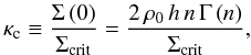
 (52)Introducing the
central convergence, κc, a parameter that determines the
lensing properties of the Einasto profile,
(52)Introducing the
central convergence, κc, a parameter that determines the
lensing properties of the Einasto profile,
 (53)we can write
 in the form
 ![Mathematical equation: \begin{equation} \alpha\left(x\right)=\frac{\kappa_{\text{c}}\,\sqrt{\pi}}{\Gamma\left(n\right)}\, x^{2}\, H_{2,3}^{2,1}\left[\begin{array}{c} (-\frac{1}{2},\,1),(0,\,1)\\ (0,\,2n),(-\frac{1}{2},\,1),(-\frac{3}{2},\,1) \end{array}\biggr|\, x^{2}\right],\label{eq:alpha-Fox} \end{equation}](/articles/aa/full_html/2012/04/aa18543-11/aa18543-11-eq124.png) (54)with a completely
analogous series expansion as for M(x). For a
spherically symmetric lens that is capable of forming multiple images of the source, one
sufficient condition is κc > 1 (Schneider et al. 1992). In the case
κc ≤ 1, only one image of the source is formed. In addition
to the condition κc > 1, multiple
images are produced only if
|y| ≤ ycrit (Li & Ostriker 2002), where
ycrit is the maximum value of y when
x < 0 or its minimum when
x > 0. For singular profiles such as an NFW
profile, the central convergence always is divergent, hence the condition
κc > 1 is always met, this implies
that an NFW profile is capable of forming multiple images for any mass. Nonsingular
profiles, such as the Einasto profile, are not capable of forming multiple images for any
mass. Instead, the condition κc > 1
sets a minimum value for lens mass required to form multiple images.
(54)with a completely
analogous series expansion as for M(x). For a
spherically symmetric lens that is capable of forming multiple images of the source, one
sufficient condition is κc > 1 (Schneider et al. 1992). In the case
κc ≤ 1, only one image of the source is formed. In addition
to the condition κc > 1, multiple
images are produced only if
|y| ≤ ycrit (Li & Ostriker 2002), where
ycrit is the maximum value of y when
x < 0 or its minimum when
x > 0. For singular profiles such as an NFW
profile, the central convergence always is divergent, hence the condition
κc > 1 is always met, this implies
that an NFW profile is capable of forming multiple images for any mass. Nonsingular
profiles, such as the Einasto profile, are not capable of forming multiple images for any
mass. Instead, the condition κc > 1
sets a minimum value for lens mass required to form multiple images.
3.3. Deflection potential
The deflection potential  for a spherically symmetric lens is given by (Schneider
et al. 1992)
for a spherically symmetric lens is given by (Schneider
et al. 1992) 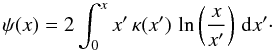 (55)Inserting Eq. (38) into (55), we obtain again a result that can be re-expressed as a Fox
H function
(55)Inserting Eq. (38) into (55), we obtain again a result that can be re-expressed as a Fox
H function
![Mathematical equation: \begin{eqnarray} \psi(x)&&=\frac{\kappa_{\text{c}}\,\sqrt{\pi}}{2\,\Gamma\left(n\right)}\, x^{3}\,\notag\\ &&\times\, H_{3,4}^{2,2}\left[\begin{array}{c} (-\frac{1}{2},\,1),(-\frac{1}{2},\,1),(0,\,1)\\ \label{eq:phi-Fox} (0,\,2n),(-\frac{1}{2},\,1),(-\frac{3}{2},\,1),(-\frac{3}{2},\,1) \end{array}\biggr|\, x^{2}\right]. \end{eqnarray}](/articles/aa/full_html/2012/04/aa18543-11/aa18543-11-eq136.png) (56)For
ψ(x) we have the same cases of expansions, a power
series for simple poles in case 1,
(56)For
ψ(x) we have the same cases of expansions, a power
series for simple poles in case 1, ![Mathematical equation: \begin{eqnarray} \psi(x)=\frac{\kappa_{\text{c}}\,\sqrt{\pi}}{2\,\Gamma\left(n\right)}\,\left[-\sum_{k=1}^{\infty}\frac{\Gamma\left(-\tfrac{3}{2}-\tfrac{k}{2n}\right)}{\Gamma\left(-\tfrac{k}{2n}\right)}\,\frac{(-1)^{k}}{k!}\,\frac{x^{k/n+3}}{3n+k}\right.\notag\\ \left.+\sum_{k=0}^{\infty}\frac{\Gamma(n-2nk)}{\Gamma\left(\tfrac{1}{2}-k\right)}\,\frac{(-1)^{k}}{(k+1)!}\,\frac{x^{2k+2}}{k+1}\right],\label{eq:phi-gen-series} \end{eqnarray}](/articles/aa/full_html/2012/04/aa18543-11/aa18543-11-eq138.png) (57)and
a logarithmic-power series for multiple poles in case 2,
(57)and
a logarithmic-power series for multiple poles in case 2,
![Mathematical equation: \begin{eqnarray} &&\psi(x) = \frac{\kappa_{\text{c}}\,\sqrt{\pi}}{2\,\Gamma\left(n\right)}\, x^{2}\,\left[\ \ -\hspace{-1.5ex}\sum_{\substack{k=1\\ k\,{\text{mod}}\, p\ne0 } }^{\infty}\hspace{-1ex}\frac{\Gamma\left(-\tfrac{3}{2}-\tfrac{k}{2n}\right)}{\Gamma\left(-\tfrac{k}{2n}\right)}\,\frac{(-1)^{k}}{k!}\,\frac{x^{k/n+1}}{3n+k}\right.\nonumber \\ &&\quad \left.+\ \frac{\Gamma(n)}{\sqrt{\pi}}\ +\ \hspace{-3ex}\sum_{\substack{k=1\\ (k+k_{0})\,{\text{mod}}\, q\ne0 } }^{\infty}\hspace{-3ex}\frac{\Gamma(n-2nk)}{\Gamma\left(\tfrac{1}{2}-k\right)}\,\frac{(-1)^{k}}{(k+1)!}\,\frac{x^{2k}}{k+1}\right]\nonumber \\ && \quad + \frac{\kappa_{\text{c}}}{2\,\Gamma\left(n\right)}\, x^{2}\,\hspace{-3ex}\sum_{\substack{k=0\\ (k+k_{0})\,{\text{mod}}\, q=0 } }^{\infty}\hspace{-3ex}\frac{(-1)^{p}\,(2k)!}{(2nk-n)!\,(k+1)!\,(k+1)!}\left(\frac{x}{2}\right)^{2k}\nonumber \\ \label{eq:phi-rat-series}&&\quad \left.\times\left[-\!\ln\left(\frac{x}{2}\right)\right.-\frac{1}{2k}+\psi(k+2)+n\,\psi(2nk-n)\!-\!\psi(2k-1)\right]. \end{eqnarray}](/articles/aa/full_html/2012/04/aa18543-11/aa18543-11-eq139.png) (58)
(58)
3.4. Magnification, shear and the critical curves
Gravitational lensing effect preserves the surface brightness but it causes variations in
shape and solid angle of the source. Therefore, the source luminosity is amplified by
(Schneider et al. 1992) 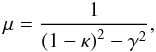 (59)where κ
is the convergence and
(59)where κ
is the convergence and  is the shear. The amplification μ has two contributions: one from the
convergence, which describes an isotropic focusing of light rays in the lens plane, and
the other which describes an anisotropic focusing caused by the tidal gravitational forces
acting on the light rays, described by the shear. For a spherical symmetric lens, the
shear is given by (Miralda-Escude 1991)
is the shear. The amplification μ has two contributions: one from the
convergence, which describes an isotropic focusing of light rays in the lens plane, and
the other which describes an anisotropic focusing caused by the tidal gravitational forces
acting on the light rays, described by the shear. For a spherical symmetric lens, the
shear is given by (Miralda-Escude 1991)
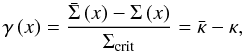 (60)where the average
surface mass density within x is
(60)where the average
surface mass density within x is 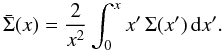 (61)The magnification
of the Einasto profile can be found combining Eqs. (38), (59)–(61). In the calculation of
(61)The magnification
of the Einasto profile can be found combining Eqs. (38), (59)–(61). In the calculation of
 ,
we use again the Mellin-Barnes integral representation (36), and integrate it to obtain an expression in terms of Fox
H function. Thus we get
,
we use again the Mellin-Barnes integral representation (36), and integrate it to obtain an expression in terms of Fox
H function. Thus we get ![Mathematical equation: \begin{equation} \mu=\left[\left(1-\bar{\kappa}\right)\left(1+\bar{\kappa}-2\kappa\right)\right]^{-1},\label{eq:magnification-einasto} \end{equation}](/articles/aa/full_html/2012/04/aa18543-11/aa18543-11-eq148.png) (62)where
(62)where ![Mathematical equation: \begin{equation} \kappa\left(x\right)=\frac{\kappa_{\text{c}}\,\sqrt{\pi}}{\Gamma\left(n\right)}\, x\, H_{1,2}^{2,0}\left[\begin{array}{c} (0,\,1)\\ (0,\,2n),(-\frac{1}{2},\,1) \end{array}\biggr|\, x^{2}\right],\label{eq:kappa-Fox} \end{equation}](/articles/aa/full_html/2012/04/aa18543-11/aa18543-11-eq149.png) (63)and
(63)and ![Mathematical equation: \begin{equation} \bar{\kappa}\left(x\right)=\frac{\kappa_{\text{c}}\,\sqrt{\pi}}{\Gamma\left(n\right)}\, x\, H_{2,3}^{2,1}\left[\begin{array}{c} (-\frac{1}{2},\,1),(0,\,1)\\ (0,\,2n),(-\frac{1}{2},\,1),(-\frac{3}{2},\,1) \end{array}\biggr|\, x^{2}\right].\label{eq:average-kappa-Fox} \end{equation}](/articles/aa/full_html/2012/04/aa18543-11/aa18543-11-eq150.png) (64)The magnification
may be divergent for some image positions. The loci of the diverging magnification in the
image plane are called the critical curves. We see from Eq. (62) that the Einasto profile has one pair of critical curves. The
first curve,
(64)The magnification
may be divergent for some image positions. The loci of the diverging magnification in the
image plane are called the critical curves. We see from Eq. (62) that the Einasto profile has one pair of critical curves. The
first curve,  ,
is the tangential critical curve, which corresponds to an Einstein Ring with a radius,
called the Einstein radius. The second curve,
,
is the tangential critical curve, which corresponds to an Einstein Ring with a radius,
called the Einstein radius. The second curve,  ,
is the radial critical curve, which also defines a ring and its corresponding radius. In
both cases the equations must be solved numerically.
,
is the radial critical curve, which also defines a ring and its corresponding radius. In
both cases the equations must be solved numerically.
4. Integer and half-integer values of n
The expressions for the Einasto surface mass density (38) and its lensing properties (42), (54), (56), (62)–(64) in terms of the Fox H
function for case n is a rational number, can be reduced to a Meijer
G function, ![Mathematical equation: \begin{eqnarray} G_{p,q}^{m,n}\left[\left.\begin{matrix}{\boldsymbol{a}}\\ {\boldsymbol{b}} \end{matrix}\,\right|\, z\right]&=&\notag\\ \label{eq:defG} &&\frac{1}{2\pi \rm i}\int_{{\cal \mathcal{L}}}\frac{\prod_{j=1}^{m}\Gamma(b_{j}+s)\prod_{j=1}^{n}\Gamma(1-a_{j}-s)}{\prod_{j=m+1}^{q}\Gamma(1-b_{j}-s)\prod_{j=n+1}^{p}\Gamma(a_{j}+s)}\, z^{-s}\,{\text{d}}s. \end{eqnarray}](/articles/aa/full_html/2012/04/aa18543-11/aa18543-11-eq153.png) (65)Meijer
G function numerical routines had been implemented in computer algebraic
systems, such as the commercial Maple, Mathematica and the free open-source Sage and mpmath
library; in contrast, there is no Fox H function implementation available.
(65)Meijer
G function numerical routines had been implemented in computer algebraic
systems, such as the commercial Maple, Mathematica and the free open-source Sage and mpmath
library; in contrast, there is no Fox H function implementation available.
For case n integer or half-integer, we can write
 as a Meijer G function. Inserting the Gauss multiplication formula (Abramowitz & Stegun 1970)
 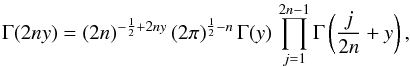 (66)into Eq. (36) and comparing with the definition (65), we obtain an expression for the surface
mass density of the Einasto profile in terms of the Meijer G function
(66)into Eq. (36) and comparing with the definition (65), we obtain an expression for the surface
mass density of the Einasto profile in terms of the Meijer G function
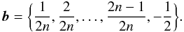
![Mathematical equation: % subequation 2186 0 \begin{equation} \Sigma(x)=\frac{\sqrt{n}\,\rho_{0}\, h}{(2\pi)^{n-1}}\, x\, G_{0,2n}^{2n,0}\left[\begin{array}{c} -\\ {\boldsymbol{b}} \end{array}\biggr|\,\frac{x^{2}}{\left(2n\right)^{2n}}\right], \end{equation}](/articles/aa/full_html/2012/04/aa18543-11/aa18543-11-eq156.png) (67a)where
b is a vector of size 2n given by
(67a)where
b is a vector of size 2n given by
 (67b)Integrating the above
expression for surface mass density according to (41) and using the integral properties of the Meijer G function
(Eq. 07.34.21.0003.01 on the Wolfram Functions Site 1),
we obtain
(67b)Integrating the above
expression for surface mass density according to (41) and using the integral properties of the Meijer G function
(Eq. 07.34.21.0003.01 on the Wolfram Functions Site 1),
we obtain ![Mathematical equation: \begin{equation} M\left(x\right)=\frac{\sqrt{n}\,\rho_{0}\, h^{3}}{2(2\pi)^{n-2}}\, x^{3}\, G_{1,2n+1}^{2n,1}\left[\begin{array}{c} -\frac{1}{2}\\ {\boldsymbol{b}},-\frac{3}{2} \end{array}\biggr|\,\frac{x^{2}}{\left(2n\right)^{2n}}\right]\cdot\label{eq:M-Meijer} \end{equation}](/articles/aa/full_html/2012/04/aa18543-11/aa18543-11-eq160.png) (68)Inserting
Eq. (65) into (49)
and performing the integral of the Meijer G function, we find
(68)Inserting
Eq. (65) into (49)
and performing the integral of the Meijer G function, we find ![Mathematical equation: \begin{equation} \alpha\left(x\right)=\frac{\kappa_{\text{c}}}{2\,(2\pi)^{n-1}\,\sqrt{n}\,\Gamma\left(n\right)}\, x^{2}\, G_{1,2n+1}^{2n,1}\left[\begin{array}{c} -\frac{1}{2}\\ {\boldsymbol{b}},-\frac{3}{2} \end{array}\biggr|\,\frac{x^{2}}{\left(2n\right)^{2n}}\right]\cdot\label{eq:alpha-Meijer} \end{equation}](/articles/aa/full_html/2012/04/aa18543-11/aa18543-11-eq161.png) (69)We obtain the deflection
potential in terms of the Meijer G function combining Eqs. (55), (65) and
again we integrate, applying the Meijer G function properties. We obtain
(69)We obtain the deflection
potential in terms of the Meijer G function combining Eqs. (55), (65) and
again we integrate, applying the Meijer G function properties. We obtain
![Mathematical equation: \begin{equation} \psi\left(x\right)=\frac{\kappa_{\text{c}}}{4\,(2\pi)^{n-1}\,\sqrt{n}\,\Gamma\left(n\right)}\, x^{3}\, G_{2,2n+2}^{2n,2}\left[\begin{array}{c} -\frac{1}{2},-\frac{1}{2}\\ {\boldsymbol{b}},-\frac{3}{2},-\frac{3}{2} \end{array}\biggr|\,\frac{x^{2}}{\left(2n\right)^{2n}}\right]\cdot\label{eq:phi-Meijer} \end{equation}](/articles/aa/full_html/2012/04/aa18543-11/aa18543-11-eq162.png) (70)The convergence can be
simply found dividing Eq. (65) by
Σcrit
(70)The convergence can be
simply found dividing Eq. (65) by
Σcrit![Mathematical equation: \begin{equation} \kappa\left(x\right)=\frac{\kappa_{\text{c}}}{2\,(2\pi)^{n-1}\,\sqrt{n}\,\Gamma\left(n\right)}\, x\, G_{0,2n}^{2n,0}\left[\begin{array}{c} -\\ {\boldsymbol{b}} \end{array}\biggr|\,\frac{x^{2}}{\left(2n\right)^{2n}}\right],\label{eq:kappa-Meijer} \end{equation}](/articles/aa/full_html/2012/04/aa18543-11/aa18543-11-eq164.png) (71)
(71)
the average convergence can be calculated by inserting Eq. (65) into Eq. (61), and then
integrating, we find ![Mathematical equation: \begin{equation} \bar{\kappa}\left(x\right)=\frac{\kappa_{\text{c}}}{2\,(2\pi)^{n-1}\,\sqrt{n}\,\Gamma\left(n\right)}\, x\, G_{1,2n+1}^{2n,1}\left[\begin{array}{c} -\frac{1}{2}\\ {\boldsymbol{b}},-\frac{3}{2} \end{array}\biggr|\,\frac{x^{2}}{\left(2n\right)^{2n}}\right]\cdot\label{eq:mean-kappa-Meijer} \end{equation}](/articles/aa/full_html/2012/04/aa18543-11/aa18543-11-eq165.png) (72)
(72)
4.1. Simple cases: n = 1 and n = 
The Einasto profile corresponding to n = 1 is a simple exponential
model, characterised by the density profile 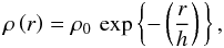 (73)the surface density
profile and lensing properties are readily found by setting n = 1 in
Eqs. (65), (68), (69), (70), (71) and (72)
(73)the surface density
profile and lensing properties are readily found by setting n = 1 in
Eqs. (65), (68), (69), (70), (71) and (72)
![Mathematical equation: \begin{eqnarray} \Sigma(x)&=&\rho_{0}\, h\, x\, G_{0,2}^{2,0}\left[\begin{array}{c} -\\ \frac{1}{2},-\frac{1}{2} \end{array}\biggr|\,\frac{x^{2}}{4}\right],\\ M\left(x\right)&=&\pi\,\rho_{0}\, h^{3}\, x^{3}\, G_{1,3}^{2,1}\left[\begin{array}{c} -\frac{1}{2}\\ \frac{1}{2},-\frac{1}{2},-\frac{3}{2} \end{array}\biggr|\,\frac{x^{2}}{4}\right],\\ \alpha\left(x\right)&=&\frac{\kappa_{\text{c}}}{2}\, x^{2}\, G_{1,3}^{2,1}\left[\begin{array}{c} -\frac{1}{2}\\ \frac{1}{2},-\frac{1}{2},-\frac{3}{2} \end{array}\biggr|\,\frac{x^{2}}{4}\right],\\ \psi\left(x\right)&=&\frac{\kappa_{\text{c}}}{4}\, x^{3}\, G_{2,4}^{2,2}\left[\begin{array}{c} -\frac{1}{2},-\frac{1}{2}\\ \frac{1}{2},-\frac{1}{2},-\frac{3}{2},-\frac{3}{2} \end{array}\biggr|\,\frac{x^{2}}{4}\right],\\ \kappa\left(x\right)&=&\frac{\kappa_{\text{c}}}{2}\, x\, G_{0,2}^{2,0}\left[\begin{array}{c} -\\ \frac{1}{2},-\frac{1}{2} \end{array}\biggr|\,\frac{x^{2}}{4}\right],\\ \bar{\kappa}\left(x\right)&=&\frac{\kappa_{\text{c}}}{2}\, x\, G_{1,3}^{2,1}\left[\begin{array}{c} -\frac{1}{2}\\ \frac{1}{2},-\frac{1}{2},-\frac{3}{2} \end{array}\biggr|\,\frac{x^{2}}{4}\right]\cdot \end{eqnarray}](/articles/aa/full_html/2012/04/aa18543-11/aa18543-11-eq169.png) The
specific Meijer G functions in these expressions can be reduced to more
standard special functions. We obtain the equivalent expressions
The
specific Meijer G functions in these expressions can be reduced to more
standard special functions. We obtain the equivalent expressions ![Mathematical equation: \begin{eqnarray} \label{eq:M-n1} \Sigma\left(x\right)&=&2\rho_{0}\, h\, x\, K_{1}\left(x\right),\label{Sigma-n1}\\ M\left(x\right)&=&8\pi\,\rho_{0}\, h^{3}\,\left[1-\frac{x^{2}}{2}\, K_{2}\left(x\right)\right],\\ \label{alpha-n1} \alpha\left(x\right)&=&\frac{4\kappa_{\text{c}}}{x}\,\left[1-\frac{x^{2}}{2}\, K_{2}\left(x\right)\right],\\ \label{eq:phi-n1} \psi\left(x\right)&=&4\kappa_{\text{c}}\left[\ln\left(\frac{x}{2}\right)+\frac{x}{2}\, K_{1}\left(x\right)+K_{0}\left(x\right)+\gamma-\frac{1}{2}\right],\\ \label{eq:kappa-n1} \kappa\left(x\right)&=&\kappa_{\text{c}}\, x\, K_{1}\left(x\right),\\ \label{eq:mean-kappa-n1} \bar{\kappa}\left(x\right)&=&\frac{4\kappa_{\text{c}}}{x^{2}}\,\left[1-\frac{x^{2}}{2}\, K_{2}\left(x\right)\right], \end{eqnarray}](/articles/aa/full_html/2012/04/aa18543-11/aa18543-11-eq170.png) where
Kν(x) is the modified
Bessel function of the second kind of order ν, and
γ ≈ 0.57721566 the Euler-Mascheroni constant. The expressions (80)–(85) can also be readily calculated by inserting the density profile (73) into the formula (24) and later carrying out all corresponding
calculations for the lensing properties.
where
Kν(x) is the modified
Bessel function of the second kind of order ν, and
γ ≈ 0.57721566 the Euler-Mascheroni constant. The expressions (80)–(85) can also be readily calculated by inserting the density profile (73) into the formula (24) and later carrying out all corresponding
calculations for the lensing properties.
For  , the
density profile (4) becomes a Gaussian,
, the
density profile (4) becomes a Gaussian,
 (86)the surface density and
lensing properties can be found through substitution of
in
Eqs. (65), (69), (68), (70), (71) and (72),
(86)the surface density and
lensing properties can be found through substitution of
in
Eqs. (65), (69), (68), (70), (71) and (72),
![Mathematical equation: \begin{eqnarray} \Sigma(x)=\sqrt{\pi}\,\rho_{0}\, h\, x\, G_{0,1}^{1,0}\left[\begin{array}{c} -\\ -\frac{1}{2} \end{array}\biggr|\, x^{2}\right],\\ M\left(x\right)=\pi^{3/2}\,\rho_{0}\, h^{3}\, x^{3}\, G_{1,2}^{1,1}\left[\begin{array}{c} -\frac{1}{2}\\ -\frac{1}{2},-\frac{3}{2} \end{array}\biggr|\, x^{2}\right],\\ \alpha\left(x\right)=\kappa_{\text{c}}\, x^{2}\, G_{1,2}^{1,1}\left[\begin{array}{c} -\frac{1}{2}\\ -\frac{1}{2},-\frac{3}{2} \end{array}\biggr|\, x^{2}\right],\\ \psi\left(x\right)=\frac{\kappa_{\text{c}}}{2}\, x^{3}\, G_{2,3}^{1,2}\left[\begin{array}{c} -\frac{1}{2},-\frac{1}{2}\\ -\frac{1}{2},-\frac{3}{2},-\frac{3}{2} \end{array}\biggr|\, x^{2}\right],\\ \kappa\left(x\right)=\kappa_{\text{c}}\, x\, G_{0,1}^{1,0}\left[\begin{array}{c} -\\ -\frac{1}{2} \end{array}\biggr|\, x^{2}\right],\\ \bar{\kappa}\left(x\right)=\kappa_{\text{c}}\, x\, G_{1,2}^{1,1}\left[\begin{array}{c} -\frac{1}{2}\\ -\frac{1}{2},-\frac{3}{2} \end{array}\biggr|\, x^{2}\right]. \end{eqnarray}](/articles/aa/full_html/2012/04/aa18543-11/aa18543-11-eq176.png) These
Meijer G function can also be written in terms of elementary and special
functions,
These
Meijer G function can also be written in terms of elementary and special
functions, ![Mathematical equation: \begin{eqnarray} \Sigma\left(x\right)=\sqrt{\pi}\rho_{0}\, h\,{\text{e}}^{-x^{2}},\label{Sigma-n-1/2}\\ M\left(x\right)=\pi^{3/2}\,\rho_{0}\, h^{3}\,\left(1-{\text{e}}^{-x^{2}}\right),\label{eq:M-n-1/2}\\ \alpha\left(x\right)=\frac{\kappa_{\text{c}}}{x}\,\left(1-{\text{e}}^{-x^{2}}\right),\label{alpha-n-1/2}\\ \psi\left(x\right)=\frac{\kappa_{\text{c}}}{2}\,\left[\ln\left(x^{2}\right)+\mathrm{E}_{1}(x^{2})+\gamma\right],\label{eq:phi-n-1/2}\\ \kappa\left(x\right)=\kappa_{\text{c}}\,{\text{e}}^{-x^{2}},\label{eq:kappa-n-1/2}\\ \bar{\kappa}\left(x\right)=\frac{\kappa_{\text{c}}}{x^{2}}\,\left(1-{\text{e}}^{-x^{2}}\right),\label{eq:mean-kappa-n-1/2} \end{eqnarray}](/articles/aa/full_html/2012/04/aa18543-11/aa18543-11-eq177.png) with
Eν(x) the exponential integral of order
ν. The above results can be easily checked by substituting Eq. (86) into recipes (24), (41), (49), (50), (55) and (61).
with
Eν(x) the exponential integral of order
ν. The above results can be easily checked by substituting Eq. (86) into recipes (24), (41), (49), (50), (55) and (61).
4.2. Profile comparison
We compared the Einasto and Sérsic surface mass densities for the same values of the Sérsic index m and Einasto index n, including the exponential and Gaussian cases. For this comparison we used the Mathematica implementation of the Meijer G function and Eq. (65). Figure 1 shows ΣS(R) for different values of m, while ΥIe and Re are held fixed; Fig. 2 displays Σ(x) for different values of n, while ρ0rs and rs are held fixed. In both figures, it can be clearly seen that the respective index is very important in determining the overall behaviour of the curves.
The Sérsic profile is characterised by a steeper central core and extended external wing for higher values of the Sérsic index m. For low values of m the central core is flatter and the external wing is sharply truncated. The Einasto profile has a similar behaviour, with the difference that the external wings are more spread out. Also in the inner region for both profiles with low values of the respectively index we obtain higher values of ΣS and Σ. Additionally, the Einasto profile has higher values of the central surface mass density than the Sérsic profile, comparing both profiles for the same index. However, the Einasto profile seems to be less sensitive to the value of the surface mass density for a given n and radius in the inner region than the Sérsic profile. It is in this region that the lensing effect is more important and the surface mass density characteristics determine the lensing properties of the respective profiles.
Given these differences between the two profiles, we clearly see that the lensing properties of Sérsic and Einasto profiles also differ, which agrees with previous work of Cardone et al. (2005) and Dhar & Williams (2010). Studies of the lensing properties of the Sérsic profile have been made by Cardone (2004) and Elíasdóttir & Möller (2007).
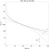 |
Fig. 1 Sérsic profile, in dimensionless units, where ΥIe and Re are held fixed for different values of the Sérsic index m. |
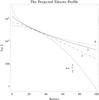 |
Fig. 2 Projected Einasto profile, where ρ0rs and rs are held fixed for different values of the Einasto index n. |
5. Asymptotic behaviour
The series expansions allow us to directly investigate the behaviour of Einasto models at
small radii. It follows that the central asymptotic behaviour of the surface density
Σ(x) depends on the value of n. If
n < 1, we find the following expansion at small
radii (x ≪ 1) ![Mathematical equation: \begin{equation} \Sigma(x)\sim\rho_{0}\, h\left[\,2\Gamma(n+1)-\Gamma(1-n)\, x^{2}\,\right]. \end{equation}](/articles/aa/full_html/2012/04/aa18543-11/aa18543-11-eq186.png) (99)If
n = 1, then the expansion has the form
(99)If
n = 1, then the expansion has the form
![Mathematical equation: \begin{equation} \Sigma(x)\sim\rho_{0}\, h\left[\,2+\left(2\ln\left(\tfrac{1}{2}\right)-1\right)\, x^{2}\,\right]. \end{equation}](/articles/aa/full_html/2012/04/aa18543-11/aa18543-11-eq187.png) (100)Finally, if
n > 1, the central surface density behaves as
(100)Finally, if
n > 1, the central surface density behaves as
![Mathematical equation: \begin{equation} \Sigma(x)\sim\rho_{0}\, h\left[\,2\Gamma(n+1)-\frac{\sqrt{\pi}}{n+1}\,\frac{\Gamma\left(\tfrac{n-1}{2n}\right)}{\Gamma\left(\tfrac{2n-1}{2n}\right)}\, x^{1+\frac{1}{n}}\,\right]. \end{equation}](/articles/aa/full_html/2012/04/aa18543-11/aa18543-11-eq189.png) (101)The behaviour of the
cumulative surface mass M(x) and deflection potential
are more straightforward. At small radii, we find the asymptotic expressions
(101)The behaviour of the
cumulative surface mass M(x) and deflection potential
are more straightforward. At small radii, we find the asymptotic expressions  (102)and
  (103)The
x2 slope for M(x) is not
unexpected, given that the Einasto models have a finite central surface mass density. The
asymptotic behaviour of the Fox H function at large radii is described in
Kilbas & Saigo (1999). We obtain the
following expansions (x ≫ 1)
(103)The
x2 slope for M(x) is not
unexpected, given that the Einasto models have a finite central surface mass density. The
asymptotic behaviour of the Fox H function at large radii is described in
Kilbas & Saigo (1999). We obtain the
following expansions (x ≫ 1)  and
and
![Mathematical equation: \begin{eqnarray} \psi(x)\sim2\,\frac{\Gamma\left(3n\right)}{\Gamma\left(n\right)}\,\kappa_{\text{c}}\,\left[\,\ln\left(\frac{x}{2}\right)-n\,\psi\left(3n\right)+1\,\right]&&\notag\\ \label{eq:Phi-large}&& +\frac{\sqrt{\pi}\,\left(2n\right)^{3/2}}{\Gamma\left(n\right)}\,\kappa_{\text{c}}\,{\text{e}}^{-x^{1/n}}\, x^{3-\frac{5}{2n}}. \end{eqnarray}](/articles/aa/full_html/2012/04/aa18543-11/aa18543-11-eq195.png) (106)
(106)
6. Summary and conclusions
We studied the spatial and lensing properties of the Einasto profile by analytical means.
For the spatial properties we applied the method used by Ciotti & Bertin (1999) to derive an analytical expansion for the
dimensionless parameter dn of the Einasto
model. We also derived analytical expressions for the cumulative mass profile
 and the gravitational potential
  .
For the lensing properties, we used the Mellin integral transform formalism to derive
closed, analytical expressions for the surface mass density
,
cumulative surface mass
.
For the lensing properties, we used the Mellin integral transform formalism to derive
closed, analytical expressions for the surface mass density
,
cumulative surface mass  ,
deflection angle ,
deflection potential ,
magnification
,
deflection angle ,
deflection potential ,
magnification  and shear
  For general values of the
Einasto index n, these are expressed in terms of the Fox H
function. Using the properties of the Fox H function, we calculated
explicit power and logarithmic-power expansions for these lensing quantities, and we
obtained simplified expressions for integer and half-integer values of n.
These series expansions allow to perform arbitrary-precision calculations of the surface
mass density and lensing properties of Einasto dark matter haloes. We also studied the
asymptotic behaviour of the surface mass density, cumulative surface mass and deflection
potential at small and large radii using the series expansions.
For general values of the
Einasto index n, these are expressed in terms of the Fox H
function. Using the properties of the Fox H function, we calculated
explicit power and logarithmic-power expansions for these lensing quantities, and we
obtained simplified expressions for integer and half-integer values of n.
These series expansions allow to perform arbitrary-precision calculations of the surface
mass density and lensing properties of Einasto dark matter haloes. We also studied the
asymptotic behaviour of the surface mass density, cumulative surface mass and deflection
potential at small and large radii using the series expansions.
Furthermore, we compared the Sérsic and Einasto surface mass densities using the equivalent values for the Sérsic m and Einasto n indices for fixed values of ΥIe, Re, ρ0rs and rs, showing that both profiles have a similar behaviour. However, we noted that for the Einasto profile the external wings are more spread out and it seems to be less sensitive than the Sérsic profile to the value of the surface mass density for a given Einasto index and radius in the inner region. Also, we find that the Einasto profile is more “cuspy” than the Sérsic profile: the former has higher values of the central surface mass density. These features are of key importance, because it is in this region that the lensing effect is more important, and these dissimilarities in the surface mass densities imply a difference in the lensing properties of both profiles. This result agrees with previous work of Cardone et al. (2005) and Dhar & Williams (2010).
Our results are the first step in studying the properties of the Einasto profile using analytical means. The constant increase of computational power opens the possibility of using more realistic and sophisticated profiles like the Einasto profile in cosmological studies, where our results may apply. For example, they can be used in strong- and weak-lensing studies of galaxies and clusters, where dark matter is believed to be the main mass component and the mass distribution can be assumed to be given by an Einasto profile. The better performance in cosmological N-body simulations of the Einasto profile (Navarro et al. 2004; Merritt et al. 2006; Gao et al. 2008; Hayashi & White 2008; Stadel et al. 2009; Navarro et al. 2010) makes its inclusion in strong and weak lensing studies very promising. Recently, Chemin et al. (2011) analysed the rotation curves (RC) of spiral galaxies from THINGS (The HI Nearby Galaxy Survey, de Blok et al. 2008) and found that the Einasto profile provides a better match to the observed RC than the NFW profile (Navarro et al. 1996, 1997) and the cored pseudo-isothermal profile. Also, Dhar & Williams (2012) modelled the surface brightness profiles of a sample of elliptical galaxies of the Virgo cluster using a multi-component Einasto profile based on an analytical approximation, and obtained a good fit for shallow-cusp and steep-cusp galaxies with fit residual errors lower in comparison to measurement errors in a wide dynamical radial range. Additionally, in their models of the most massive galaxies, the outer components are characterised by being in the range 5 ≲ n ≲ 8, and a comparable range is obtained from N-body simulations for the Einasto profile. Our exact analytical results for the spatial and lensing properties of the Einasto may be used to constrain the value of the Einasto index and determine if the galaxy or cluster studied is dark matter dominated or not. More studies like Chemin et al. (2011) and Dhar & Williams (2012) could help to strengthen the position of the Einasto profile as a new standard model for dark matter haloes. Also, increasing the use of the Einasto profile in new cosmological studies could provide progress towards a solution to the cusp-core problem.
This paper continues the effort initiated by Baes & Gentile (2011) and Baes & van Hese (2011) to advocate the use of the Fox H and Meijer G functions in theoretical astrophysics, in particular for studying the analytical properties of density models like the Sérsic model, where no additional analytical progress could be made until the Mellin integral transform formalism was applied. We hope that our work has again demonstrated the usefulness of the Fox H and Meijer G functions as tools for analytical work.
Acknowledgments
E.R.M. and F.F.A. wish to thank H. Morales and R. Carboni for critical reading. This research has made use of NASA’s Astrophysics Data System Bibliographic Services. G.G. is a postdoctoral researcher of the FWO-Vlaanderen (Belgium). Moreover, we would like to thank the referee for valuable suggestions on the manuscript.
References
- Abramowitz, M., & Stegun, I. A. 1970, Handbook of mathematical functions (Dover) [Google Scholar]
- Adamchick, V. 1996, Mathematica in Education and Research, 5, 16 [Google Scholar]
- Andredakis, Y. C., Peletier, R. F., & Balcells, M. 1995, MNRAS, 275, 874 [NASA ADS] [CrossRef] [Google Scholar]
- Anguita, T., Faure, C., Kneib, J.-P., et al. 2009, A&A, 507, 35 [NASA ADS] [CrossRef] [EDP Sciences] [Google Scholar]
- Baes, M., & Gentile, G. 2011, A&A, 525, A136 [NASA ADS] [CrossRef] [EDP Sciences] [Google Scholar]
- Baes, M., & van Hese, E. 2011, A&A, 534, A69 [NASA ADS] [CrossRef] [EDP Sciences] [Google Scholar]
- Banerjee, A., Matthews, L. D., & Jog, C. J. 2010, New A, 15, 89 [Google Scholar]
- Bartelmann, M. 1996, A&A, 313, 697 [NASA ADS] [Google Scholar]
- Bartelmann, M., & Schneider, P. 2001, Phys. Rep., 340, 291 [NASA ADS] [CrossRef] [Google Scholar]
- Binney, J., & Tremaine, S. 1987, Galactic dynamics (Princeton University Press) [Google Scholar]
- Boyarsky, A., Neronov, A., Ruchayskiy, O., & Tkachev, I. 2010, Phys. Rev. Lett., 104, 191301 [NASA ADS] [CrossRef] [PubMed] [Google Scholar]
- Burkert, A. 1995, ApJ, 447, L25 [NASA ADS] [CrossRef] [Google Scholar]
- Caon, N., Capaccioli, M., & D’Onofrio, M. 1993, MNRAS, 265, 1013 [NASA ADS] [CrossRef] [Google Scholar]
- Cardone, V. F. 2004, A&A, 415, 839 [NASA ADS] [CrossRef] [EDP Sciences] [Google Scholar]
- Cardone, V. F., Piedipalumbo, E., & Tortora, C. 2005, MNRAS, 358, 1325 [NASA ADS] [CrossRef] [Google Scholar]
- Cardone, V. F., Del Popolo, A., Tortora, C., & Napolitano, N. R. 2011, MNRAS, 416, 1822 [NASA ADS] [CrossRef] [Google Scholar]
- Cellone, S. A., Forte, J. C., & Geisler, D. 1994, ApJS, 93, 397 [NASA ADS] [CrossRef] [Google Scholar]
- Chae, K.-H., Turnshek, D. A., & Khersonsky, V. K. 1998, ApJ, 495, 609 [NASA ADS] [CrossRef] [Google Scholar]
- Chemin, L., de Blok, W. J. G., & Mamon, G. A. 2011, AJ, 142, 109 [NASA ADS] [CrossRef] [Google Scholar]
- Ciotti, L. 1991, A&A, 249, 99 [NASA ADS] [Google Scholar]
- Ciotti, L., & Bertin, G. 1999, A&A, 352, 447 [NASA ADS] [Google Scholar]
- Ciotti, L., & Lanzoni, B. 1997, A&A, 321, 724 [NASA ADS] [Google Scholar]
- Clowe, D., Bradač, M., Gonzalez, A. H., et al. 2006, ApJ, 648, L109 [NASA ADS] [CrossRef] [Google Scholar]
- Davies, J. I., Phillipps, S., Cawson, M. G. M., Disney, M. J., & Kibblewhite, E. J. 1988, MNRAS, 232, 239 [NASA ADS] [CrossRef] [Google Scholar]
- de Blok, W. J. G. 2010, Adv. Astron., 2010 [Google Scholar]
- de Blok, W. J. G., McGaugh, S. S., Bosma, A., & Rubin, V. C. 2001, ApJ, 552, L23 [NASA ADS] [CrossRef] [Google Scholar]
- de Blok, W. J. G., Walter, F., Brinks, E., et al. 2008, AJ, 136, 2648 [NASA ADS] [CrossRef] [Google Scholar]
- Dhar, B. K., & Williams, L. L. R. 2010, MNRAS, 405, 340 [NASA ADS] [Google Scholar]
- Dhar, B. K., & Williams, L. L. R. 2012, MNRAS, accepted [arXiv:1112.3120] [Google Scholar]
- Donato, F., Gentile, G., & Salucci, P. 2004, MNRAS, 353, L17 [NASA ADS] [CrossRef] [MathSciNet] [Google Scholar]
- Donato, F., Gentile, G., Salucci, P., et al. 2009, MNRAS, 397, 1169 [NASA ADS] [CrossRef] [Google Scholar]
- Donnarumma, A., Ettori, S., Meneghetti, M., et al. 2011, A&A, 528, A73 [NASA ADS] [CrossRef] [EDP Sciences] [Google Scholar]
- D’Onofrio, M., Capaccioli, M., & Caon, N. 1994, MNRAS, 271, 523 [NASA ADS] [CrossRef] [Google Scholar]
- Einasto, J. 1965, Tartu Astron. Obs. Teated, 17, 1 [NASA ADS] [Google Scholar]
- Einasto, J. 1969a, Astron. Nachr., 291, 97 [NASA ADS] [CrossRef] [Google Scholar]
- Einasto, J. 1969b, Astrophysics, 5, 67 [NASA ADS] [CrossRef] [Google Scholar]
- Einasto, J. 1974, in Stars and the Milky Way System, ed. L. N. Mavridis, 291 [Google Scholar]
- Elíasdóttir, Á., & Möller, O. 2007, J. Cosmology Astropart. Phys., 7, 6 [Google Scholar]
- Fikioris, G. 2007, Mellin Transform Method for Integral Evaluation: Introduction and Applications to Electromagnetics (Morgan & Claypool) [Google Scholar]
- Gadotti, D. A. 2009, MNRAS, 393, 1531 [NASA ADS] [CrossRef] [Google Scholar]
- Gao, L., Navarro, J. F., Cole, S., et al. 2008, MNRAS, 387, 536 [NASA ADS] [CrossRef] [Google Scholar]
- Gentile, G., Salucci, P., Klein, U., Vergani, D., & Kalberla, P. 2004, MNRAS, 351, 903 [NASA ADS] [CrossRef] [MathSciNet] [Google Scholar]
- Gentile, G., Burkert, A., Salucci, P., Klein, U., & Walter, F. 2005, ApJ, 634, L145 [NASA ADS] [CrossRef] [Google Scholar]
- Gentile, G., Salucci, P., Klein, U., & Granato, G. L. 2007, MNRAS, 375, 199 [NASA ADS] [CrossRef] [Google Scholar]
- Gentile, G., Famaey, B., Zhao, H., & Salucci, P. 2009, Nature, 461, 627 [NASA ADS] [CrossRef] [PubMed] [Google Scholar]
- Graham, A. W., & Driver, S. P. 2005, PASA, 22, 118 [NASA ADS] [CrossRef] [Google Scholar]
- Graham, A. W., & Guzmán, R. 2003, AJ, 125, 2936 [NASA ADS] [CrossRef] [Google Scholar]
- Graham, A. W., Merritt, D., Moore, B., Diemand, J., & Terzić, B. 2006, AJ, 132, 2711 [NASA ADS] [CrossRef] [Google Scholar]
- Hayashi, E., & White, S. D. M. 2008, MNRAS, 388, 2 [NASA ADS] [CrossRef] [Google Scholar]
- Hoekstra, H., Yee, H. K. C., & Gladders, M. D. 2004, ApJ, 606, 67 [NASA ADS] [CrossRef] [Google Scholar]
- Huang, Z., Radovich, M., Grado, A., et al. 2011, A&A, 529, A93 [NASA ADS] [CrossRef] [EDP Sciences] [Google Scholar]
- Jee, M. J., Rosati, P., Ford, H. C., et al. 2009, ApJ, 704, 672 [NASA ADS] [CrossRef] [Google Scholar]
- Jing, Y. P., & Suto, Y. 2000, ApJ, 529, L69 [NASA ADS] [CrossRef] [PubMed] [Google Scholar]
- Kaiser, N., & Squires, G. 1993, ApJ, 404, 441 [NASA ADS] [CrossRef] [Google Scholar]
- Keeton, C. R. 2002, ApJ, 575, L1 [NASA ADS] [CrossRef] [Google Scholar]
- Keeton, C. R. 2003, ApJ, 582, 17 [NASA ADS] [CrossRef] [Google Scholar]
- Keeton, C. R., & Madau, P. 2001, ApJ, 549, L25 [NASA ADS] [CrossRef] [Google Scholar]
- Keeton, C. R., & Zabludoff, A. I. 2004, ApJ, 612, 660 [NASA ADS] [CrossRef] [Google Scholar]
- Kilbas, A. A., & Saigo, M. 1999, J. Appl. Math. Stochast. Anal., 12, 191 [Google Scholar]
- Kilbas, A. A., & Saigo, M. 2004, H-Transforms: Theory and Applications (CRC Press) [Google Scholar]
- Kochanek, C. S., Blandford, R. D., Lawrence, C. R., & Narayan, R. 1989, MNRAS, 238, 43 [NASA ADS] [CrossRef] [Google Scholar]
- Kochanek, C. S., Falco, E. E., Impey, C. D., et al. 2000, ApJ, 535, 692 [NASA ADS] [CrossRef] [Google Scholar]
- Kormendy, J., & Freeman, K. C. 2004, in Dark Matter in Galaxies, ed. S. Ryder, D. Pisano, M. Walker, & K. Freeman, IAU Symp., 220, 377 [Google Scholar]
- Li, L.-X., & Ostriker, J. P. 2002, ApJ, 566, 652 [NASA ADS] [CrossRef] [Google Scholar]
- Li, N., & Chen, D.-M. 2009, Res. Astron. Astrophys., 9, 1173 [NASA ADS] [CrossRef] [Google Scholar]
- Limousin, M., Richard, J., Kneib, J.-P., et al. 2008, A&A, 489, 23 [NASA ADS] [CrossRef] [EDP Sciences] [Google Scholar]
- Mahdavi, A., Hoekstra, H., Babul, A., Balam, D. D., & Capak, P. L. 2007, ApJ, 668, 806 [NASA ADS] [CrossRef] [Google Scholar]
- Mamon, G. A., & Łokas, E. L. 2005, MNRAS, 362, 95 [NASA ADS] [CrossRef] [Google Scholar]
- Marichev, O. I. 1982, Handbook of Integral Transforms of Higher Transcendental Functions: Theory and Algorithmic Tables (Chichester: Horwood) [Google Scholar]
- Mathai, A. M. 1978, The H-function with applications in statistics and other disciplines (Wiley) [Google Scholar]
- Mathai, A., Saxena, R., & Haubold, H. 2009, The H-Function: Theory and Applications (Springer) [Google Scholar]
- Mazure, A., & Capelato, H. V. 2002, A&A, 383, 384 [NASA ADS] [CrossRef] [EDP Sciences] [Google Scholar]
- Mellier, Y. 1999, ARA&A, 37, 127 [NASA ADS] [CrossRef] [Google Scholar]
- Merritt, D., Graham, A. W., Moore, B., Diemand, J., & Terzić, B. 2006, AJ, 132, 2685 [NASA ADS] [CrossRef] [Google Scholar]
- Miralda-Escude, J. 1991, ApJ, 370, 1 [NASA ADS] [CrossRef] [Google Scholar]
- Möllenhoff, C., & Heidt, J. 2001, A&A, 368, 16 [NASA ADS] [CrossRef] [EDP Sciences] [Google Scholar]
- Moore, B., Quinn, T., Governato, F., Stadel, J., & Lake, G. 1999, MNRAS, 310, 1147 [NASA ADS] [CrossRef] [Google Scholar]
- Morandi, A., Limousin, M., Rephaeli, Y., et al. 2011, MNRAS, 1336 [Google Scholar]
- Moriondo, G., Giovanardi, C., & Hunt, L. K. 1998, A&AS, 130, 81 [NASA ADS] [CrossRef] [EDP Sciences] [Google Scholar]
- Napolitano, N. R., Romanowsky, A. J., & Tortora, C. 2010, MNRAS, 405, 2351 [NASA ADS] [Google Scholar]
- Navarro, J. F., Frenk, C. S., & White, S. D. M. 1996, ApJ, 462, 563 [NASA ADS] [CrossRef] [Google Scholar]
- Navarro, J. F., Frenk, C. S., & White, S. D. M. 1997, ApJ, 490, 493 [NASA ADS] [CrossRef] [Google Scholar]
- Navarro, J. F., Hayashi, E., Power, C., et al. 2004, MNRAS, 349, 1039 [NASA ADS] [CrossRef] [Google Scholar]
- Navarro, J. F., Ludlow, A., Springel, V., et al. 2010, MNRAS, 402, 21 [NASA ADS] [CrossRef] [Google Scholar]
- Oguri, M., Bayliss, M. B., Dahle, H., et al. 2012, MNRAS, 420, 3213 [NASA ADS] [CrossRef] [Google Scholar]
- Primack, J. R. 2003, Nucl. Phys. B Proc. Suppl., 124, 3 [Google Scholar]
- Prugniel, P., & Simien, F. 1997, A&A, 321, 111 [NASA ADS] [Google Scholar]
- Salucci, P., & Burkert, A. 2000, ApJ, 537, L9 [NASA ADS] [CrossRef] [Google Scholar]
- Sand, D. J., Treu, T., & Ellis, R. S. 2002, ApJ, 574, L129 [NASA ADS] [CrossRef] [Google Scholar]
- Schneider, P., Ehlers, J., & Falco, E. E. 1992, Gravitational Lenses, ed. P. Schneider, J. Ehlers, & E. E. Falco [Google Scholar]
- Sereno, M., & Umetsu, K. 2011, MNRAS, 416, 3187 [NASA ADS] [CrossRef] [Google Scholar]
- Sérsic, J. L. 1968, Atlas de galaxias australes, ed. J. L. Sérsic [Google Scholar]
- Simon, J. D., Bolatto, A. D., Leroy, A., Blitz, L., & Gates, E. L. 2005, ApJ, 621, 757 [NASA ADS] [CrossRef] [Google Scholar]
- Spano, M., Marcelin, M., Amram, P., et al. 2008, MNRAS, 383, 297 [NASA ADS] [CrossRef] [Google Scholar]
- Springel, V., White, S. D. M., Jenkins, A., et al. 2005, Nature, 435, 629 [NASA ADS] [CrossRef] [PubMed] [Google Scholar]
- Springel, V., Wang, J., Vogelsberger, M., et al. 2008, MNRAS, 391, 1685 [NASA ADS] [CrossRef] [Google Scholar]
- Stadel, J., Potter, D., Moore, B., et al. 2009, MNRAS, 398, L21 [NASA ADS] [CrossRef] [Google Scholar]
- Swaters, R. A., Madore, B. F., van den Bosch, F. C., & Balcells, M. 2003, ApJ, 583, 732 [NASA ADS] [CrossRef] [Google Scholar]
- Trujillo, I., Graham, A. W., & Caon, N. 2001, MNRAS, 326, 869 [NASA ADS] [CrossRef] [Google Scholar]
- Umetsu, K., Broadhurst, T., Zitrin, A., et al. 2011, ApJ, 738, 41 [NASA ADS] [CrossRef] [Google Scholar]
- van den Bosch, F. C., & Swaters, R. A. 2001, MNRAS, 325, 1017 [NASA ADS] [CrossRef] [Google Scholar]
- Walker, M. G., McGaugh, S. S., Mateo, M., Olszewski, E. W., & Kuzio de Naray, R. 2010, ApJ, 717, L87 [NASA ADS] [CrossRef] [Google Scholar]
- Wambsganss, J., & Paczynski, B. 1994, AJ, 108, 1156 [NASA ADS] [CrossRef] [Google Scholar]
- Weldrake, D. T. F., de Blok, W. J. G., & Walter, F. 2003, MNRAS, 340, 12 [NASA ADS] [CrossRef] [Google Scholar]
- Zhao, H. 1996, MNRAS, 278, 488 [Google Scholar]
- Zitrin, A., Broadhurst, T., Coe, D., et al. 2011a, MNRAS, 413, 1753 [NASA ADS] [CrossRef] [Google Scholar]
- Zitrin, A., Rosati, P., Nonino, M., et al. 2011b, ApJ, submitted [arXiv:1107.2649] [Google Scholar]
All Figures
|
Fig. 1 Sérsic profile, in dimensionless units, where ΥIe and Re are held fixed for different values of the Sérsic index m. |
| In the text | |
|
Fig. 2 Projected Einasto profile, where ρ0rs and rs are held fixed for different values of the Einasto index n. |
| In the text | |
Current usage metrics show cumulative count of Article Views (full-text article views including HTML views, PDF and ePub downloads, according to the available data) and Abstracts Views on Vision4Press platform.
Data correspond to usage on the plateform after 2015. The current usage metrics is available 48-96 hours after online publication and is updated daily on week days.
Initial download of the metrics may take a while.