| Issue |
A&A
Volume 540, April 2012
|
|
|---|---|---|
| Article Number | A18 | |
| Number of page(s) | 12 | |
| Section | The Sun | |
| DOI | https://doi.org/10.1051/0004-6361/201118163 | |
| Published online | 16 March 2012 | |
Morphology of the quiet Sun between 150 and 450 MHz as observed with the Nançay radioheliograph
LESIA-Observatoire de Paris, CNRS, UPMC, Univ. Paris-Diderot, France
e-mail: This email address is being protected from spambots. You need JavaScript enabled to view it.
; This email address is being protected from spambots. You need JavaScript enabled to view it.
Received: 27 September 2011
Accepted: 27 January 2012
Abstract
Context. Since its last upgrading in 2004, the Nançay radioheliograph (NRH) is able to produce reliable images of the quiet Sun in the 150–450 MHz range, which corresponds to the low and medium corona. These images are better than those previously obtained with the NRH or other instruments in this range and are suitable for quantitative and systematic exploitation.
Aims. We aim to study the radio aspects of the solar atmosphere. We aim to focuss on the description of the morphology and the comparisons with observations in EUV and X-ray ranges and with magnetic structures.
Methods. We used the rotational aperture synthesis technique (suitable for non time-varying objects) along with an original self-calibration procedure and a specific deconvolution algorithm (a variant of CLEAN that includes a scale analysis).
Results. We present results from radio imaging of the quiet Sun with the NRH. The analysis was carried over about 160 days during the summers (June-August) from 2004 to 2011. We confirms and extend our first results, which were published from a much smaller data sample. We emphasize new aspects of the corona observed in this frequency range, in particular the existence of coronal holes darker than previously reported and dark channels at high frequencies. We give examples that illustrate the complex morphology of coronal structures as revealed by radio imaging, the center-to-limb effects (radio occultation) and the variation with the phase of the solar cycle. We compare our images with large-scale coronal magnetic structures. We show that dark coronal holes and channels seen at high frequencies and bright ribbons seen at low frequencies seem to be associated with particular types of magnetic structures.
Conclusions. Detailed radio images in this frequency range are a new tool with high potential for investigating the low and middle corona, since these images can emphasize structures that are not (or much less) visible at other wavelengths. In the near future, there is much to learn from observations with NRH during the ascending part of the cycle (never observed at m/dcm wavelengths ) and from composite images of combined NRH and GMRT data, which will have a much better resolution. In a second step, it will be interesting to obtain circularly polarized images (giving a diagnostic of the coronal magnetic field) and images with new-generation instruments, which will yield detailed images with shorter synthesis or even snapshot images, from which processes evolving on shorter time scales can be studied.
Key words: Sun: corona / Sun: radio radiation / Sun: chromosphere
© ESO, 2012
1. Introduction
There are two techniques for observing the outer solar atmosphere on the disk. The first technique is the observation in the EUV or soft X-ray range. Thanks to several satellites presently in operation, this is now the main source of information on the corona. Among others, it daily provides a wealth of images with high spatial, spectral, and temporal resolutions. The choice of the wavelengths determines the temperature range of observed regions. However, because the emission is optically thin and weighted by the square of the density, the images are dominated by the lower and denser parts of visible structures. Except close to active regions (ARs) where high coronal loops are observed, the middle and upper corona are difficult to observe.
The second technique is radio observations. In contrast with EUV and soft X-ray observations, they allow us to observe the corona in a wide range of altitudes, all the higher because the observing frequency f is low. A first reason for this is that radio waves at frequency f cannot propagate in regions in which f > fp, where  is the plasma frequency and ne the electron density, which decreases with altitude. Observations at f are thus blind to contributions of regions where fp > f. Emission at f < 1 GHz comes only from regions where ne < 1010 cm-3, that is, from the transition region and corona (the smaller f, the higher the emission level), and emission at f < 100 MHz comes only from regions where ne < 108 cm-3, roughly above 0.5 solar radius (Rs). A second reason is that if we exclude non-thermal emissions related to flare or ARs, the relevant emission mechanism for frequencies <1 GHz is the free-free thermal emission. The absorption coefficient
  , where ξ is the Coulomb logarithm, μ the refraction index (lower at low frequencies and in dense regions) and T the electron temperature. The optical depth τ of the corona is >1 for f between ≈60 and ≈200 MHz. At these frequencies the only contribution is from the corona. Above 300 MHz, τ decreases and rays penetrate to the transition region. However, it is widely believed that the transition region is too thin to produce a significant contribution.
In contrast, the radio observations have the following limitations:
-
they require interferometers with kilometric size in themeter-to-decimeter (m/dcm) wavelength range to obtain aresolution of 1 arcmin or less;
-
because the quiet Sun (QS) is a complex source with a wide spectrum of spatial scales, the number of antennas is generally too small to obtain snapshot images that satisfactorily describe all structures. For this reason, rotational synthesis technique (RST) is often used for QS studies, which requires the absence of rapidly varying non-thermal radio emissions;
-
the production of reliable images requires both good calibration and deconvolution.
These limitations explain why radio imaging of the Sun in the m/dcm λ range was not widely used up to now, although this technique was developed before EUV observations.
In the m/dcm range, only few instruments can produce usable images of the QS. The early studies involved the one-dimensional (1D) interferometer at 169 MHz in Nançay (Axisa et al. 1971). A few 2D images at 80 and 160 MHz using the Culgoora radioheliograph (decomissioned in 1986) were reported by Dulk & Sheridan (1974). More 2D images were obtained later with an early version (2 × 1D) of the Nançay radioheliograph (NRH) at 169 MHz (Alissandrakis et al. 1985). Some 2D images were also obtained with the Clark Lake radioheliograph (CLRO) between 1982 and 1989 in the decameter range (73 MHz and below). The RATAN 600 telescope is always in operation but is only 1D and observes at 600 MHz and above. The Very Large Array (VLA) can produce RST images, but it is not dedicated to the Sun, which precludes a long series of observations, and it has been very rarely used for imaging the Sun at 327 and 1421 MHz. After 1996, the NRH (primarily designed for bursts studies) was improved in several steps and became more suitable for imaging the QS:
-
it became indeed 2D (instead of 2 × 1D) in 1996 (Kerdraon & Delouis1997) and observed at five then six frequencies between 150 and450 MHz;
-
it was completed in 2003 (unpublished) with four additional anti-aliasing antennas giving a better uv coverage for short baselines;
-
the number of observed frequencies was increased from 6 to 10 in 2008, to improve the spectral description.
Using these last improvements and a newly developed calibration procedure, Mercier & Chambe (2009, hereafter MC), produced images with better quality than previously published.
The QS emission has been reviewed in the dcm/m range by Lantos (1980, 1998), Alissandrakis (1994), and in the mm/dam range by Shibasaki et al. (2011). Decades of observations have shown that the radio Sun is a non-uniform and variable source, traditionally described as consisting of three components: 1) a wide background, the QS, involving only large scales on the order of 1 Rs and slowly varying with the solar cycle, 2) a slowly varying component (SVC), classically described as the emission of a few of localized regions with sizes less than a few arc minutes, superimposed on the QS and varying over time scales from one day to several weeks, 3) non-thermal continua and bursts, generally much brighter. They imply time scales from less than one second to tens of minutes for bursts, and up to several days for continua. Both generally show a strong circular polarization, whereas the QS and SVC are unpolarized or weakly polarized at NRH frequencies. Bursts are not addressed in this paper.
It has been found that the QS is wider in the EW than in the NS direction, with a progressive decrease of the brightness toward the edges, and it is generally wider than the optical disk, except in the NS direction for frequencies above 300 and up 450 MHz (data are missing between 450 and 1000 MHz). Its brightness temperature Tb and its size increase with the wavelength and reach their maximum during cycle maximum. It should be noted that Tb is lower and the size is larger than expected from optical and EUV observations.
The SVC results both from thermal sources and faint noise storm continua. These storms can be distinguished thanks to their polarization and the presence of bursts. They are generally more compact and brighter than the thermal sources and are systematically located near ARs. At 408 MHz, the consensus is that thermal sources coincide with ARs or faculae. It was first claimed (Moutot & Boischot 1961; Leblanc 1970) that this was also the same at 160 MHz. It was then soon established that ARs are only poorly visible at 160 MHz. This was explained in terms of too high density for these structures. Indeed, most thermal sources at low frequencies were observed far from ARs, and their association with optical features remained unclear. Axisa et al. (1971), using a large database (300 cases) from 1D observations at Nançay, concluded that thermal sources at 169 MHz were located above Hα filaments, at the base of the associated streamers. This was corroborated from very few cases by Dulk & Sheridan (1974) from 2D observations at Culgoora. Lang & Willson (1989), using the VLA, also reported some sources at 327 MHz that were overlaid on filaments. Through a series of papers based on 2D NRH images, Alissandrakis, Lantos, and co-workers found that thermal sources were almost never associated with Hα filaments, but were more or less related to the photospheric inversion lines revealed by spatially averaged magnetograms. However, these authors did not reach a clear conclusion: thermal sources at 169 MHz span the inversion line and there is no clear relation with streamers at the limb (Alissandrakis et al. 1985); later, no conclusion for sources visible at 169 MHz only was derived (Lantos et al. 1992); a statistical analysis showed that sources at 169 MHz are above or very near inversion lines (with a distribution peaking at distances of 4–6 deg) but not associated with filaments (Alissandrakis & Lantos 1996); sources at 169 MHz are in regions of enhanced K-corona emission (Lantos & Alissandrakis 1996); most of sources at 169 MHz are located between faculae and inversion lines, some of them being close to inversion lines (Lantos & Alissandrakis 1999).
The same authors (Lantos et al. 1992) introduced the concept of a coronal plateau and confirmed it (Alissandrakis 1994; Lantos & Alissandrakis 1996; Lantos 1998; Lantos & Alissandrakis 1999). It was defined as a quasi-uniform area, brighter (ΔTb = 50 − 100 kK) than the average QS, surrounding all local emission sources and running “around the Sun in a continuous manner”, and it was considered the dominant feature of the large-scale coronal emission. The plateau had a close association with the zone of enhanced K-corona emission and was identified “with the diffuse emission of a high-altitude loop system which overrides the principal inversion line of the general magnetic field at the base of the heliosheet” (Shibasaki et al. 2011).
During the seventies, it appeared that radio coronal features could be in depression. Coronal holes in radio were first reported from Culgoora observations at 160 and 80 MHz by Dulk & Sheridan (1974), then afterward at 169 and 408 MHz at Nançay (Alissandralis et al. 1985; Lantos et al. 1992; Alissandrakis 1994; Lantos 1998; Lantos & Alissandrakis 1999). These radio holes appear as brightness depressions, approximately corresponding to holes visisble in EUV. They show more contrast at 408 MHz (about 50% of the QS) than at lower frequencies. Most of them are still visible at 169 MHz as shallow depressions (10–20%), more rarely at 80 MHz and at lower frequencies, where they can occasionally appear as faint brightness enhancements (Lantos et al. 1987). Because of the limited resolution and dynamic range in images, the shapes in radio and EUV could not be precisely compared.
Narrow brightness depressions associated with large Hα filaments were reported at mm and cm wavelengths by Chiuderi-Drago (1990) and at 6 and 21 cm with the VLA (Kundu et al. 1985). Depressions longer than Hα filaments and corresponding to photospheric inversion lines are currently observed at 17 GHz in the daily images from the Nobeyama radioheliograph, although with a low contrast. From a systematic study, Marqué (2004) concluded that elongated depressions at 408 MHz were associated with Hα filaments and could occasionally be observed at lower frequencies. These depressions are often longer than the filaments themselves. Their shape was continuous even if filaments were not, and had a close correspondence with that of EUV channels. They are commonly referred to as filament channels.
It must be noted that several of the concepts used above (e.g. QS, thermal sources) are derived from the picture of the radio corona developed during the early observations with limited instruments. For instance, the concept of QS is difficult to specify. It was proposed (before holes were clearly observed in radio) to define the QS as the minimum envelope of images during a sufficiently long period (e.g. a year). Because coronal holes are generally darker than their surroundings, this leads to define the QS as the lowest brightness in coronal holes, which is not satisfactory since coronal holes are essentially open field regions, whereas most emission of the QS comes from closed loops. We also point out that at m/dcm wavelengths only a small number of radio images (often below 200 MHz) are available in the literature, and that most of them consist of isocontour plots, which are not very suitable for a good description of details. Moreover, observations were rarely made simultaneously at different frequencies.
The recent results of MC with the NRH were derived from a limited database over the period 2004–2008, with an extent comparable to that of previous studies. They can be summarized as follows:
-
the radio corona has a morphology more complex than previouslydescribed. Structures have a wide spectrum of spatial scales andare often highly contrasted, especially at the highest NRHfrequencies;
-
brightness temperatures Tb in coronal holes above 400 MHz are lower (down to ≈ 100 kK) than previously accepted ( ≈ 400 kK);
-
the aspect of the corona changes with the solar cycle between 2004 and 2008.
The first point shows that it is necessary to reconsider several of the historical concepts. However, this requires a comprehensive morphological study and a detailed comparison with other data, which was not achieved by MC. The aim of the present paper is to present such a description from a larger database and to investigate the relations between radio and magnetic features.
2. Observations, data processing, and selection
Observations and data processing were made with the last improvements of the NRH described by MC. We used several criteria to select the data. First, we restricted ourselves to observations between May and August, when the uv coverage is better and ionospheric disturbances effects are at their minimum. Second, we eliminated days with obvious instrumental or radio frequencies interference problems. Finally, days with intense non-thermal activity were also eliminated.
However, selecting only totally quiet days would have led to an unsufficient data set. For quite a few of the many observations affected by moderate activity, this activity was confined within time intervals that could be excised from data. An automatic procedure to do this was defined as follows. The time variation of the total flux is not sensitive enough, since the flux is mainly due to the QS, except for very strong bursts. However, for baselines longer than a few hundreds of meters, even small bursts can exceed the contribution of the QS. We considered the annular domain D in the uv plane defined by  where
where  and
and  , and d = 50 m is the shortest baseline of the NRH. The inner boundary was empirically chosen for eliminating short baselines dominated by the QS, and the outer one ensures that D remains within the region of dense uv coverage. For each set of instantaneous data, we then calculated the mean value M over D of the modulus of the complex visibility (CV). This mean value M was found to be a better activity indicator than the flux. We excluded from the synthesis time intervals for which M exceeds its “quiet level” by more than a specified factor a. Taking a = 1.1 or 1.2 gave satisfactory results. The corresponding reduction in the uv coverage resulted in a somewhat degraded dirty image, but the cleaned image was only slightly affected. We were sometimes led to accept data with a somewhat higher activity level for interesting. This produced defects on the image, that were generally localized near the active region.
We eventually selected 160 days, which is by far more than for any previous studies on 2D images. Their distribution is indicated in Fig. 1. They are about 50% of the usable days between 2004 and 2008, and a smaller fraction in 2009, 2010, and 2011.
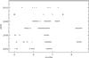 |
Fig. 1 Selected days: the beginning of months is indicated in the abscissa. |
3. Results
Considering the few examples presented in previous studies and the better quality of our images, it is useful to display here a sufficiently meaningful sample of cases to illustrate the various aspects of the morphology of the radio corona.
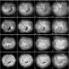 |
Fig. 2 Examples of the Sun during the decay of cycle 23 for 2004–2007 (from top to bottom) at four frequencies between 432 and 150 MHz. Dates and frequencies (decreasing from left to right) are indicated in each frame. Fields of view are 2.8 Rs, intensity scales are linear, resolutions are indicated by small disks at the lower left corner of each frame. Rows are referred to as a, b, c, and d in the text (same for following figures). |
3.1. Morphology of the radio Sun between 150 and 450 MHz
The results presented here confirm and extend those of MC, who had shown that the aspect of the Sun depends both on the observing frequency and the phase of the solar cycle. Figures 2 and 3 present images of the Sun at four frequencies for one typical day in each year from 2004 to 2011. Figure 4 gives an example of the Sun at eight frequencies in 2010. In this section, we merely describe the various solar structures as they appear in radio images. We will compare them with structures visible from other data in Sects. 4.3 and 4.4.
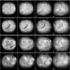 |
Fig. 3 Examples of the Sun at minimum and beginning of cycle 24 for 2008–2011 (from top to bottom) at 4 frequencies between 445 and 150 MHz. Dates and frequencies (decreasing from left to right) are indicated in each frame. |
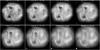 |
Fig. 4 The Sun at eight frequencies between 445 and 150 MHz (decreasing from left to right and from top to bottom) on 2010 May 15. |
3.1.1. Changes with frequency
Images at extreme frequencies of NRH are usually fairly different. The changes are progressive with frequency, all the more so because successive frequencies are close to each other. The observations at six frequencies (2004–2007) often showed substantial changes between successive frequencies, especially below 327 MHz. Observations at ten frequencies (2008–2011) give a better spectral description (see Fig. 4, where only eight frequencies are shown), but because of TV broadcasting, we have no observations at frequencies between 228 and 173 MHz, a relatively wide interval. This may partially explain why below 230 MHz the changes can be abrupt over this range.
At high frequencies (HF, 408–445 MHz) the corona is highly contrasted. The brightest areas are associated with ARs. They consist of small patches that can produce extended complexes (e.g. June 29, 2004, in Fig. 2a).
The darkest features are low-latitude coronal holes. Coronal holes (even small ones) are much darker than the disk, with brightness temperature Tb in the range 80–200 kK, compared to typically 400 kK on the disk. At HF, the holes are not uniform but show a marked structure, with darker pits and brighter peaks that can be recognized at close frequencies, especially for observations at ten frequencies. This internal structure gradually disappears below 300–350 MHz, and the position of holes shows a progressive shift from middle to low frequencies. Large holes generally remain visible during their transit across the disk for about 1 week. In some cases, they could be followed for nine consecutive days, while in some other cases they are not visible for more than four days around their transit at central meridian, although they can be observed one solar rotation before or after.
Other conspicuous HF features are elongated, dark, or bright. Dark channels are the longest visible coronal structures, with lengths up to 2 Rs. They have Tb ≈ 200−300 kK and can be partially bordered by edges with a more or less pronounced brightening. They can remain visible for about one week or more during their transit and can be recognized after one or more solar rotations. In some cases, they extend far from holes, but in other cases they encircle the holes more or less completely. In these last cases, their borders become particularly bright (Fig. 2d). Dark channels also generally become less visible as the frequency decreases, with some progressive position shifts as well, while some of them, however, are more visible at intermediate frequencies.
At low frequencies (LF, 164–150 MHz) the contrast is weaker. Holes are much less visible, disappear or even become brighter than their surroundings. The most conspicuous features are bright areas or elongated ribbons with Tb exceeding its typical value of 600 kK on the disk by up to 300 kK. It must be noted that they do not correspond to the brightest areas visible at HF, but often to regions with moderate brightness at HF (e.g. June 29, 2004 in Fig. 2a and June 01, 2004 in Fig. 7a).
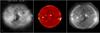 |
Fig. 5 The Sun on June 27, 2004, observed with NRH at 432 MHz (left) with NoRH at 17 GHz (middle) and in X-rays with SXI (right). The contrast in the NoRH image was enhanced and the brightest areas in the SXI image were saturated. |
3.1.2. Changes with solar cycle
Our database now covers a large part of the solar cycle, from the beginning of the decay in 2004 to the growth of the present cycle, and clearly shows that the aspect of the corona depends on the phase of the cycle. The overall size of the Sun at all frequencies is smaller during minimum (Fig. 3a and b) both in EW and NS directions.
Large-scale dark structures, such as large coronal holes or long channels, which are common in 2004–2005 (Fig. 2a, b), become less frequent during 2006 and 2007, practically disappear during the minimum in 2008–2009 (Fig. 3a), and clearly reappear in 2010–2011 (Fig. 3c, d). This is especially true for the long channels. Some low-latitude coronal holes, however, are observed in 2008-2009, but they are either small or fragmented (Fig. 3b). The corona seems then to be organized on a large scale around the hole (Fig. 3b).
In contrast, images at frequencies above about 350 MHz exhibit many small patches during minimum (Fig. 3a, b), with typical size 1–2′ of arc, either brighter or darker than the mean disk by about 5 × 10⁴ K and lasting generally for no more than one day. Among the presently available images, they first appear in June 2007, are quite common in 2008–2009 and are no longer observed in 2010 and 2011. To our knowledge, these small structures have not been previously reported.
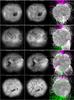 |
Fig. 6 Comparison between radio images at 432 MHz and magnetic features for four days (from top to bottom). From left to right: the radio image, then superimposed with the WSO magnetogram (middle) and the PFSS plot (right). Dates are indicated in radio images. Rows are referred to as a, b, c, and d in the text (same for the next figure). |
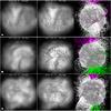 |
Fig. 7 Comparison between radio images at 50 or 164 MHz and magnetic features for three days (same as for the preceding figure). |
3.2. Comparison with other images
At radio frequencies, in addition to the NRH, only the Siberian Solar Radio Telescope (SSRT) and the Nobeyama radioheliograph (NoRH) produce daily images of the Sun, but at much shorter wavelengths. The SSRT images at 5.7 GHz show ARs and their close surroundings, but no details on the disk. The NoRH images at 17 GHz show more details but are quite different from the NRH ones because the corresponding emission levels lie at much lower altitudes. Figure 5 gives an example, reproduced from MC for convenience. In the NoRH image, the radio Sun is practically limited to the visible disk, and the contrast (excepting ARs) is actually lower than with the NRH, although we enhanced it in the presented NoRH image. Coronal holes (in particular the large one) are not visible and the long dark channel is only slightly visible.
When compared to the EUV or X-ray images, the NRH images show some similitude at the highest frequencies, but reveal quite different structures at the lowest frequencies.
3.3. Comparison with the magnetic field and Hα data
Because the radio observations between 150 and 450 MHz reveal aspects of the corona from low levels up to ≈ 0.5 Rs, we need a description of the magnetic field in the same height range. Because the magnetic structure becomes more and more simple with altitude (with only one neutral magnetic sheet in the interplanetary medium), we used coronal extrapolations of the photospheric field and smoothed magnetograms at photospheric level from the Wilcox Solar Observatory (WSO). Because we aim to derive general qualitative rules concerning the association between radio and magnetic structures, simplified PFSS extrapolations are sufficient and we used the extrapolations plots given by the PFSSviewer code provided by DeRosa that is available in the SolarSoftware. We merely recall that this field is probably between the photosphere and a “source surface”, usually set at the central distance 2.5 Rs, where it becomes radial.
We produced superposition of radio images and WSO magnetograms and PFSS plots for about 100 days over the period 2004–2010. Because the WSO magnetograms are derived from observations made 8–12 h after the NRH observations, we first corrected them for the solar rotation. We focus here only on the most remarkable and large-scale features in radio images: a) dark features at HF (holes or elongated channels), b) bright areas or ribbons at LF. It rapidly appeared that the correspondence between radio and magnetic structures was more or less clear according to the phase of the solar cycle. In 2004, the cycle was only beginning to decline and PFSS plots showed clear magnetic structuring on the disk with, for instance, arcades (long systems of medium-scale arches with axes roughly normal to the plane of arches) and large extended unipolar regions of an open and diverging magnetic field. There was a trend for these structures to become more and more random up to the minimum of the cycle in 2008–2009, and to partially reappear in 2010 and 2011. We found that simple rules could be derived from clear examples in 2004, the validity of which could be checked (sometimes less clearly) for almost all other days in the following years. These rules can be summarized as follows:
3.3.1. Coronal holes
Our comparison between radio images and PFSS plots confirms that coronal holes are associated with open field areas. Figure 6 give examples. The correspondence is generally good, but
-
limits of open field areas on PFSS plots may not fully coincidewith limits of holes in radio at HF;
-
holes, by definition, are always bordered with arch-like closed fields. In some places of PFSS plots, these closed fields involve large-scale and dense arch systems, sharply limited at the border of the hole. We did not find any clear radio counterpart to these arch systems;
-
in some cases, the PFSS plots do not reveal open field lines. Figure 6d shows an example: between June 15 and 24, 2007, the coronal hole, clearly visible in radio, is not associated with open field lines in PFSS plots.
Some dark and elongated regions are associated with open fields. They are thus coronal holes, but they are difficult to distinguish, from radio data only, from the majority of dark channels (referred to just below), which are associated with clearly different magnetic features.
3.3.2. Dark channels
Most often, dark channels (at low latitude or in the polar crown) are associated with inversion lines in magnetograms and low arcade systems in PFSS plots. Figure 6 gives examples. The association generally holds during their entire transit on the disk. Dark channels are well-defined and smooth features in radio images, but the reliability of their association with magnetic features depends on the aspect of the inversion lines in WSO magnetograms and also on the aspect of PFSS plots. The association is less good when inversion lines have complicated or sawtooth-like shapes and/or when PFSS plots are difficult to read because many high-altitude field lines hide regular low-latitude arcades. To check this point, we used Hα filaments as proxies of magnetic inversion lines. Every time a filament was present, as seen in images from the global Hα network, it matched the dark channel even when this did not coincide with the WSO inversion line. Dark channels at HF are often bordered by bright and narrow ribbons (Fig. 6d) that likely correspond to footpoints of arches.
In some cases, dark channels associated with inversion lines point toward a coronal hole: in Fig. 6b (May 08, 2004) the eastern dark channel turns to the end of the elongated hole near the center of the disk, and in Fig. 6c (June 25, 2004) the very long dark channel connects at the SE end of the large hole.
3.3.3. Low-frequency bright areas
When the LF brightenings described in 4.2.1 are particularly pronounced, they more or less completely fill regions limited by inversion lines but systematically avoid the inversion lines themselves. The arcades overriding the inversion lines are regular and the intermediate unipolar region does not include open field lines, as revealed by the PFSS plots (Fig. 7). Now, the magnetic topology of two parallel arcades without intermediate open field lines is that of a pseudo-streamer (Wang et al. 2007a). The presence of a pseudo-streamer seems to be a necessary condition for a strong and elongated LF brightening to occur since we found no case for which such a brightening follows a large-scale magnetic loop.
The LF bright areas can be also the counterpart of holes that appear dark at frequencies <250 MHz, but in these cases the brightness is less than when enclosed by inversion lines.
After we found that the most conspicuous bright areas at LF coincide with pseudo-streamers, we tried for the sake of completeness to identify the radio signature of streamers. Streamers correspond to coronal regions located between two holes of opposite polarities. In PFSS plots, they appear as regions of high magnetic loops overriding the only inversion line between these holes. In most of these cases, we found that one of the two holes was a polar one and that consequently streamers are essentially high-latitude structures. Although they are not particularly bright and hence not noticeable on the disk at LF, they have a clear signature at the limb where they appear as radial extensions of the corona. An example is shown in Fig. 7c for May 27, 2004, near the SE limb.
Thus, whereas the brightest regions on the disk at LF are associated with pseudo-streamers, large and moderately bright radial extensions of the corona at high latitudes are associated with streamers.
All rules described in Sect. 3.3 are valid in the vicinity of the disk center. Some departures may be observed near the limbs, where perspective and refraction effects are stronger. As mentioned at the beginning of this section, when the solar cycle declines after 2004, these rules may be less clearly verified. We explain this with the lower confidence level of magnetograms and PFSS plots, which become less and less ordered and reliable as the magnetic intensity decreases. The association with radio features become more and more difficult but the above rules are never clearly disproved. Another limitation in estimating their validity is that in the immediate surroundings of ARs, the radio brightness is affected by the presence of hot and dense regions, which renders the identification of dark channels difficult.
4. Discussion
Compared with earlier QS studies with the NRH, our work relies on images with an improved and more homogeneous quality, on more processed days (160) spread over eight years, and on more (six, then ten) simultaneous frequencies.
We showed that the corona appears as a complex radio source and cannot be described in terms of a smooth background completed with a few localized bright and dark areas. At all the NRH frequencies, the corona exhibits a variety of scales, from more than 1 Rs (long dark channels, large holes at HF, elongated bright areas at LF) down to the resolution limit (small holes, fine structure in large holes, transverse dimension of dark channels, bright spots in particular near cycle minimum). It was already known from a few observations that the aspect of the corona was not the same at 408 and 169 MHz (Shibasaki et al. 2011). We showed that this aspect progressively changes from high to low frequencies, with a loss of contrast (in particular for coronal holes) from 450 down to 230 MHz and that a marked transition occurs below 230 MHz. Structures then become fairly different and the most conspicuous ones are bright areas, often elongated as bright ribbons. Unfortunately, we had no observations between 228 and 173 MHz because of TV broadcasting and it was not possible to better describe the transition in the morphology. Anyway, the clear difference in images at 450 and 150 MHz illustrates the ability of radio observations to reveal different structures in the low and medium corona according to the observation frequency, in contrast with the EUV, as mentioned in Sect. 1.
In the past, relations between optical and m/dcm radio features were investigated. One clear result from our study is that these relations can exist but are not the rule: the comparison with large-scale magnetic structures is more relevant and allows one to derive relatively simple rules, at least in a first step.
At HF, we confirmed earlier results that the brightest areas are associated with ARs. We found that they may have a complex fine structure (Fig. 2b) which makes a detailed comparison difficult.
At LF (169 MHz), Axisa et al. (1971) had found an association between bright regions and Hα filaments from low-resolution 1D images. This was not confirmed by Alissandrakis, Lantos, and co-workers from 2D images at 169 MHz with a better resolution. Through a series of papers, these authors found no significant correlation between bright regions and Hα filaments and suspected a relation with one inversion line of spatially averaged photospheric magnetograms, but they gave no clear conclusion for this relation. We found that bright regions at 164 MHz are in fact limited by two or more inversion lines, or by a single folded-up line. Thus, bright regions could be close to inversion lines but they systematically avoid them. These lines define an inner region with only one magnetic polarity which, when a low-frequency brightening is present, contains no open flux. If this region lies between two regions (necessarily with the same polarity) that both include open fluxes, the whole structure is basically that of a pseudo-streamer, as described by Wang et al. (2007a,b). A possible explanation of this disagreement with the results of Axisa et al. (1971) is that, given the complexity usually revealed by our 2D images, the faint 1D bumps identified by these authors on smooth 1D backgrounds were either not significant or not associated with only one bright region.
There are prominent dark features, especially at the highest frequencies: dark channels and holes. Our images with a high resolution and dynamic range show that the limits of holes at HF are sharp and that they coincide most of the time with those seen in EUV and, to a lesser extent, in the PFSS extrapolations. We extend, based on more data, the results of MC: holes are darker than previously reported. For instance at 408–445 MHz, their brightness temperature is currently <150 kK and not about 400 kK, as compiled by Lantos (1998) or reported by Chiuderi-Drago et al. (1999).
Marqué (2004) considered those dark channels at 408 MHz that were associated with filaments. He showed that these channels were longer, more continuous, and wider than the filaments, and closely associated with inversion lines. He identified them with the filament channels. We found that dark channels (regardless of the presence or absence of Hα filaments) generally coincide with inversion lines (or equivalently with the central part of long and low magnetic arcades on the PFSS plots), both of which are often much longer than filaments. This allows us to distinguish them from elongated holes, which appear quite similar on images but are unambiguously associated with open field lines in PFSS plots.
These results, derived from periods where the Sun exhibited a clear magnetic structuring, hold for most cases. We find that the correspondence between radio features and magnetic structures of the low or middle corona is more relevant than the correspondence with high-altitude structures such as the heliosheet, which was considered by Lantos et al. (1972) and Alissandrakis (1994). The corona observed in radio at our frequencies is still too complex to be compared with the relatively simple magnetic structure at the base of the interplanetary medium, where there is generally only one inversion line.
There are, however, exceptions to our rules. In some cases there was a discrepancy between dark channels and the inversion line of the spatially averaged magnetograms. In such cases, if an Hα filament was present, we found that it coincided with a part of the dark channel. Since Hα filaments are considered as reliable markers of inversion lines, we conclude that these discrepancies do not contradict our rule but rather question the reliability of the used magnetograms. It will be interesting to resume the study with more sensitive magnetic observations. We also observed several examples of dark channels that apparently connect with holes. However, inversion lines cannot in principle connect to holes that are considered as simple unipolar regions. Therefore, either the association of dark channels with inversion lines close to holes should be reconsidered, or holes must involve bipolar areas, at least near their border. In the same way, in spite of the generally good correspondence between the limits of holes in EUV and at 400–450 MHz, there are sometimes small but significant differences between these limits, for instance an additional small bay on one of the two structures. Both these last points should be investigated more closely with more sensitive magnetic measurements and a better resolution.
Another result of our study comes from the period covered by the observations: we were able to continuously describe the changes in the morphology over eight years in the 150–450 MHz range for the first time. The most spectacular changes concern the highest frequencies: large-scale structures (large holes, long dark channels) are prominent and show a high contrast from 2004 to 2007 (although in May, 2007, the disk shows relatively low contrast). Dark channels practically disappear in 2008–2009. During this period we observed small-scale structures (both bright and dark) above 400 MHz, which were never reported before. No conclusion could be drawn on their association with magnetic structures, because neither the PFSS extrapolations nor the spatially averaged WSO magnetograms showed significant structures. At these small scales, such an association could only be searched for by using high-resolution magnetograms. Large-scale features reappeared in 2010–2011, but not with the same aspect.
The changes are similar but less marked at 150–173 MHz, where bright large-scale structures are always visible, although with a reduced contrast.
Finally, we question the concept of coronal plateau introduced by Lantos et al. (1992). For about 20 representative days, we tried to identify a plateau in our images at 408 and 164 MHz, following the definition given by these authors. We considered two isocontours separated by ΔTb = 100 kK around a central value Tbmean. We tried, by varying Tbmean, to make the area between these contours appear as “a wide belt running as far as possible around the Sun”, according to the picture given by the authors. We failed to find any example of such a plateau: In most cases, the delimited area showed no clear behavior: during the cycle minimum (2008–2009) it covered most of the disk with many holes (in the usual meaning of the word). We then compared its shape with that of the inversion line, using the GONG magnetogram synoptic maps available in archives (after 2006). For all days but one, there was no correspondence, and in the last case only a very partial one. We conclude that the coronal plateau probably does not exist above 150 MHz. In addition, what Lantos and co-workers call “streamer belt” is in fact the brightest region in synoptic maps of the K-corona at 1.3 Rs. Because the radio emission at 164 MHz is produced at comparable heights, it is not surprising that most of bright regions in radio images are in this zone, but this altitude is too low to see only streamers. Moreover, the resolution in longitude on these synoptic maps is low, hardly less than 1 Rs, and no precise comparisons in position can be made, whereas they are possible on the disk with magnetograms.
This study should be completed over an entire solar cycle. As mentioned above, several specific points remain open and should be investigated with more detailed magnetic data.
5. Summary and conclusion
Using a larger database, we confirmed the main results of MC, listed at the end of Sect. 1. We also gave a more complete description of the radio corona and investigated new points.
The general morphology of the corona seen by the NRH is highly structured and implies a variety of spatial scales. The morphology is different at HF and LF.
At HF (>400 MHz) the three main components are active regions, holes, and elongated structures (dark or bright):
-
The existence of bright radio counterparts of active regions at HFwas already known. When several active regions are close eachother, they appear as a unique bright area.
-
Holes are clearly visible. MC reported large holes, with brightness temperatures down to Tb ≈ 100 kK, lower than previously reported. We found that large holes are non-uniform, with minimum Tb ranging from 80 to 200 kK and local maxima brighter by about 200 kK. We also found that some holes are narrow and elongated (e.g. Fig. 6b), with an aspect similar to that of dark channels, and that small compact holes can be very dark.
-
Elongated structures with small transverse extent (≈0.1 Rs) are very common, which is a new result of this work. They appear either as dark channels (e.g. Figs. 2a, d and 3c) with lengths 0.3–2.0 Rs (e.g. Fig. 6b and c), or as bright ribbons encircling holes (Fig. 6d). Dark channels can be bordered by brighter banks (e.g. Fig. 6d).
At low frequencies (<200 MHz), the aspect of corona is different:
-
We confirm that active regions are generally no longer visible andthat holes are hardly visible, either slightly darker or brighter thantheir surroundings, or even not visible at all. When visible, theyare smaller than at high frequencies, have smoother boundariesand show a progressive outward position-shift when they are farfrom the center of the disk.
-
We find that dark channels are also visible at low frequencies, although there are generally not so many and they do not always correspond to those visible at high frequencies. They appear wider than at high frequencies, but this may be partly a resolution effect.
-
Our main result is that the brightest regions are the most remarkable structures and have large extents, i.e. they cannot be described as local sources, as in earlier studies. We find that they often appear as bright ribbons, but wider than what could be explained by the limited resolution, with lengths up to 1 Rs and Tb exceeding that of the mean disk by 200–300 kK.
Therefore, elongated structures have an essential role in the structure of the corona at high and low frequencies. The transition in the aspect between high and low frequencies is progressive, although structures at the extreme frequencies of the NRH generally do not correspond for a given day. In spite of a lack of observations between 228 and 173 MHz, it seems that there is a transition in the aspect of the corona below 200 MHz, where bright ribbons become the most prominent structures.
We specify the changes in the aspect of the corona with solar cycle, outlined by MC and which concern mainly high frequencies: during cycle minimum, large-scale structures (holes and channels) essentially disappear and small-scale and short-lived structures are visible above 350 MHz. These structures were observed between June 2007 and August 2009. In 2010 and 2011 large-scale structures reappear, but with an aspect somewhat different from that of 2004–2007.
New results of the present study concern the association of structures in radio images and large-scale magnetic features as shown in spatially averaged magnetograms and PFSS plots. At high frequencies, radio holes have sharp boundaries, which in general correspond closely to those of EUV holes. They are associated with open-field areas in PFSS plots. Most of the long dark channels are associated with inversion lines seen in spatially averaged magnetograms and with systems of low arcades in PFSS plots. In this case they are just the filament channels reported by previous authors. However, some of them are long and narrow coronal holes. At low frequencies, bright regions cover areas limited by inversion lines (but not overriding them) and are associated with magnetic structures similar to that of pseudo-streamers.
In conclusion, the radio corona has a complex structure: even outside active regions and coronal holes, that is, on the main part of the disk surface, the corona is structured. The historical concepts of QS, coronal plateau, and localized sources are inadequate for a convenient description. We had already shown that the structure of the CV in the uv plane is complex and has small-scale features (see Fig. 6 in Shibasaki et al. 2011) and requires a dense uv coverage to be properly described. It follows that radio imaging is difficult but, when performed simultaneously at several frequencies, is a promising tool for investigating the 3D structure of the corona. From this study, it appears that advances in the subject could be made if observations are improved with a wider coverage in frequency and/or a better resolution.
For instance, holes show more internal structure and are darker at 400–450 MHz than at lower frequencies. It would therefore be interesting to investigate the tendency at higher frequencies. There are presently no observations between 450 and 1000 MHz, but in the near future, the Chinese Spectro-Radioheliograph (CSRH) will observe above 600 MHz. These observations will also be useful to investigate if small-scale bright structures such as are observed at 400–450 MHz during cycle minimum also exist at higher frequencies during other stages of the cycle. If so, these structures could then be the radio counterpart of bright points observed in EUV. A better resolution would be helpful for investigating what seems to be a connection between holes and dark channels, and also the structure of complex brightening at high frequencies close to active regions.
Similarly, observations at frequencies lower than150 MHz are needed for several reasons. Holes can be either darker or brighter than the mean disk at 150 MHz, and the question of their aspect at lower frequencies remains open. Do they systematically become brighter than the disk at low frequencies, as seen by Lantos et al. (1987) in one case observed at 37 and 75 MHz with the CLRO radioheliograph? It would also be interesting to investigate whether the bright elongated structures we observe at 150 MHz present a different aspect at still lower frequencies. Does a coronal plateau appear at lower frequencies? Observations at low frequencies could be possible, in a relatively near future, with the Murchison array and LOFAR.
Observations at frequencies ≈200 MHz with the NRH should be soon possible, as a consequence of reallocation of frequencies in the TV band. This will help to better describe the change in the morphology of coronal structures at this frequency.
Finally, it is of interest to look for a limit in the fine structure of the radio corona, which could give some insight on the scattering process of radio waves on coronal inhomogeneities. A joint study between the NRH and the GMRT is presently in progress, with the aim to produce rotational synthesis images resulting from the uv coverage of both instruments, as already done by Mercier et al. (2006) for snapshot imaging of bursts. An improvement in the resolution by a factor of 3–5 at 150, 236 and 327 MHz is expected.
Acknowledgments
Wilcox Solar Observatory data used in this study was obtained via the web site http://wso.stanford.edu, courtesy of J. T. Hoeksema. The Wilcox Solar Observatory is currently supported by NASA. The PFSS plots used in this study were obtained by using the PFSS viewer routine, available in the IDL Solar Software, courtesy of M. L. DeRosa.
References
- Alissandrakis, C. E. 1994, Adv. Space Res., 14, 81 [NASA ADS] [CrossRef] [Google Scholar]
- Alissandrakis, C. E., & Lantos, P. 1996, Sol. Phys., 165, 61 [NASA ADS] [CrossRef] [Google Scholar]
- Alissandrakis, C. E., & Lantos, P. 1999, A&A, 351, 373 [NASA ADS] [Google Scholar]
- Alissandrakis, C. E., Lantos, P., & Nicolaidis, E. 1985, Sol. Phys., 97, 267 [NASA ADS] [CrossRef] [Google Scholar]
- Axisa, F., Avignon, Y., Martres, M.-J., Pick, M., & Simon, P. 1971, Sol. Phys., 165, 161 [Google Scholar]
- Chiuderi-Drago, F., Landi, E., Fludra, A., & Kerdraon, A. 1999, A&A, 348, 261 [NASA ADS] [Google Scholar]
- Dulk, G. A., & Sheridan, K. V. 1974, Sol. Phys., 36, 191 [NASA ADS] [CrossRef] [Google Scholar]
- Kerdraon, A., & Delouis, J.-M. 1997, in Coronal Physics from Radio and Space Observations, Proceedings of the CESRA workshop held in Nouan le Fuzelier, ed. G. Trottet (Berlin: Springer), 192 [Google Scholar]
- Kundu, M. R., Gergely, T. E., Schmahl, E. L., et al. 1987, Sol. Phys., 108, 113 [NASA ADS] [CrossRef] [Google Scholar]
- Lang, K. R., & Willson, R. F. 1989, A&A, 199, 325 [NASA ADS] [Google Scholar]
- Lantos, P. 1980, in Radio physics of the Sun, ed. M. R. Kundu, & T. E. Gergely, Proc. IAU Symp., 86, 41 [Google Scholar]
- Lantos, P. 1999, in Proceedings of Nobeyama Symposium, held in Kiyosato Japan, Oct. 27–30, 1998, ed. T. S. Bastian, N. Goplaswamy, & K. Shibasaki, NRO Report No. 479, 11 [Google Scholar]
- Lantos, P., & Alissandrakis, C. E. 1996, Sol. Phys., 165, 83 [NASA ADS] [CrossRef] [Google Scholar]
- Lantos, P., & Alissandrakis, C. E. 1999, A&A, 351, 373 [NASA ADS] [Google Scholar]
- Lantos, P., Alissandrakis, C. E., Gergely, T. E., & Kundu, M. R. 1987, Sol. Phys., 112, 325 [NASA ADS] [CrossRef] [Google Scholar]
- Lantos, P., Alissandrakis, C. E., & Rigaud, D. 1992, Sol. Phys., 137, 225 [Google Scholar]
- Marqué, C. 2004, ApJ, 602, 1037 [NASA ADS] [CrossRef] [Google Scholar]
- Mercier, C., & Chambe, G. 2009, ApJ, 700, L137 [NASA ADS] [CrossRef] [Google Scholar]
- Mercier, C., Subramanian, P., Kerdraon, A., et al. 2006, A&A, 447, 1189 [Google Scholar]
- Shibasaki, K., Alissandrakis, C. E., & Pohjolainen, S. 2011, Sol. Phys., 272, 309 [NASA ADS] [CrossRef] [Google Scholar]
- Wang, Y.-M., Sheeley, N. R. Jr., & Rich, N. B. 2007a, ApJ, 658, 1340 [NASA ADS] [CrossRef] [Google Scholar]
- Wang, Y.-M., Bierstaker, J. B., Sheeley, N. R. Jr, et al. 2007b, ApJ, 660, 882 [NASA ADS] [CrossRef] [Google Scholar]
All Figures
|
Fig. 1 Selected days: the beginning of months is indicated in the abscissa. |
| In the text | |
|
Fig. 2 Examples of the Sun during the decay of cycle 23 for 2004–2007 (from top to bottom) at four frequencies between 432 and 150 MHz. Dates and frequencies (decreasing from left to right) are indicated in each frame. Fields of view are 2.8 Rs, intensity scales are linear, resolutions are indicated by small disks at the lower left corner of each frame. Rows are referred to as a, b, c, and d in the text (same for following figures). |
| In the text | |
|
Fig. 3 Examples of the Sun at minimum and beginning of cycle 24 for 2008–2011 (from top to bottom) at 4 frequencies between 445 and 150 MHz. Dates and frequencies (decreasing from left to right) are indicated in each frame. |
| In the text | |
|
Fig. 4 The Sun at eight frequencies between 445 and 150 MHz (decreasing from left to right and from top to bottom) on 2010 May 15. |
| In the text | |
|
Fig. 5 The Sun on June 27, 2004, observed with NRH at 432 MHz (left) with NoRH at 17 GHz (middle) and in X-rays with SXI (right). The contrast in the NoRH image was enhanced and the brightest areas in the SXI image were saturated. |
| In the text | |
|
Fig. 6 Comparison between radio images at 432 MHz and magnetic features for four days (from top to bottom). From left to right: the radio image, then superimposed with the WSO magnetogram (middle) and the PFSS plot (right). Dates are indicated in radio images. Rows are referred to as a, b, c, and d in the text (same for the next figure). |
| In the text | |
|
Fig. 7 Comparison between radio images at 50 or 164 MHz and magnetic features for three days (same as for the preceding figure). |
| In the text | |
Current usage metrics show cumulative count of Article Views (full-text article views including HTML views, PDF and ePub downloads, according to the available data) and Abstracts Views on Vision4Press platform.
Data correspond to usage on the plateform after 2015. The current usage metrics is available 48-96 hours after online publication and is updated daily on week days.
Initial download of the metrics may take a while.