| Issue |
A&A
Volume 540, April 2012
|
|
|---|---|---|
| Article Number | A58 | |
| Number of page(s) | 5 | |
| Section | Catalogs and data | |
| DOI | https://doi.org/10.1051/0004-6361/201118123 | |
| Published online | 27 March 2012 | |
Washington photometry of 26 moderately young small angular size clusters in the Large Magellanic Cloud⋆
Instituto de Astronomía y Física del Espacio, CC 67, Suc. 28, 1428 Ciudad de Buenos Aires, Argentina
e-mail: andres@iafe.uba.ar
Received: 19 September 2011
Accepted: 13 February 2012
Aims. With the aim of enlarging the number of studied LMC clusters in the age range 8.0 ≲ log(t) ≲ 9.0, we focus here on a sample of mostly unstudied cluster candidates.
Methods. We present for the first time CCD Washington CT1T2 photometry of stars in the field of 26 LMC clusters.
Results. The studied clusters turned out to be small angular size objects with ages within the age range 8.0 ≲ log(t) ≲ 9.0, which are projected or immersed in dense star fields.
Key words: techniques: photometric / galaxies: star clusters: general / galaxies: individual: LMC
Full Table 2 is only available in electronic form at the CDS via anonymous ftp to cdsarc.u-strasbg.fr (130.79.128.5) or via http://cdsarc.u-strasbg.fr/viz-bin/qcat?J/A+A/540/A58
© ESO, 2012
1. Introduction
The period ranging between log(t) ~ 8.0 and 9.0 in the Large Magellanic Cloud (LMC) star cluster formation has had different interesting results. These include the following: i) de Grijs & Anders (2006, see their Fig. 6) show that during this age range the least-squares power-law fit to the fading, non-disrupted clusters, for a constant ongoing cluster formation rate (CFR) crosses the disruption lines for the age ranges where disruption most likely dominates evolutionary fading; ii) Pandey et al. (2010) studied the integrated magnitudes and colours for LMC clusters from synthetic models and find that the magnitude and colour fluctuations are lower in this age range; and iii) Harris & Zaritsky (2009, see their Fig. 11) subdivided the time axis of the LMC star formation rate (SFR) into three segments; the middle panel covering the same age range, thus making this LMC epoch particularly relevant.
We estimate for the first time the fundamental parameters based on Washington photometry for 26 of the mostly unstudied LMC clusters whose ages are within the presently considered range. The paper is organized as follows. Section 2 describes the analysis of the 26 poorly studied LMC clusters, whereas Sect. 3 summarizes our results.
2. Fundamental parameters of poorly studied clusters
Star clusters in the LMC.
CT1T2 data of stars in the field of NGC 2093.
Piatti (2011, performed a search within the National Optical Astronomy Observatory (NOAO) Science Data Management (SDM) Archives1 looking for Washington photometric data towards the LMC. He found images corresponding to 21 different fields spread throughout the LMC obtained at the Cerro-Tololo Inter-American Observatory (CTIO) 4 m Blanco telescope with the Mosaic II camera attached (36′ × 36′ field onto a 8K × 8K CCD detector array). We assume that the area covered by these 21 Mosaic II fields represents an unbiased subsample of the LMC as a whole. They encompass 214 catalogued star clusters (Bica et al. 2008).
When examining their colour-magnitude diagrams (CMDs) and colour-colour diagrams, we found 36 clusters older than 1 Gyr (see P11), 26 clusters with some sign of evolution (present studied sample), 62 very young clusters, and 90 asterisms. Since we are interested in clusters with 8.0 ≲ log(t) ≲ 9.0, we focus herein on the second group of 26 identified clusters. As far as we are aware, none of these clusters have published CT1T2 photometry. Table 1 summarizes the information we gathered.
We reduced the data following the procedures documented by the NOAO Deep Wide Field Survey team (Jannuzi et al. 2003) and utilized the mscred package in IRAF2. We performed overscan, trimming and cross-talk corrections and bias subtraction, obtained an updated world coordinate system (WCS) database, flattened all data images, once the calibration frames (zeros, sky- and dome- flats, etc.) were properly combined. We measured nearly 90 independent standard stars from the list of Geisler (1996) per filter for each night in order to secure the transformation from the instrumental to the standard system. We solved the transformation equations with the fitparams task in IRAF and found mean colour terms of − 0.090 ± 0.003 in C, − 0.020 ± 0.001 in T1 (R) and 0.060 ± 0.004 in T2 (I), while typical airmass coefficients resulted in 0.31, 0.09, and 0.06 for C, T1, and T2, respectively. The nightly rms errors from the transformation to the standard system were 0.021, 0.023, and 0.017 mag for C, T1, and T2, respectively, indicating these nights had excellent photometric quality.
We performed the stellar photometry by using the star-finding and point-spread-function (PSF) fitting routines in the DAOPHOT/ALLSTAR suite of programs (Stetson et al. 1990). For each frame, we derived a quadratically varying PSF by fitting ~ 960 stars, once we eliminated the neighbours using a preliminary PSF derived from the brightest, least contaminated ~ 240 stars. We seleced both groups of PSF stars interactively. We then used the ALLSTAR program to apply the resulting PSF to the identified stellar objects and to create a subtracted image which was used to find and measure the magnitudes of additional fainter stars. This procedure was repeated three times for each frame. Finally, we standardized the resulting instrumental magnitudes and combined all the independent measurements using the stand-alone DAOMATCH and DAOMASTER programs, kindly provided by Peter Stetson. The final information gathered for each cluster consisted of a running number per star of the x and y coordinates, of the measured T1 magnitudes and C − T1 and T1 − T2 colours, and of the observational errors σ(T1), σ(C − T1) and σ(T1 − T2). The T1 magnitude and C − T1 and T1 − T2 colour errors provided by DAOPHOT II are shown in Fig. 1, where we only plotted the errors for stars measured in the central region (r = 30″) of NGC 2039 – the most populated cluster of the sample – to emphasize crowding effects. Only a portion of the Washington data for NGC 2093 is shown here (see Table 2) for guidance regarding their form and content. The whole Washington data for these studied clusters can be obtained as supplementary material on the on-line version of the journal.
We produced the cluster radial profiles shown in Fig. 2, which helped us adopt representative cluster radii in the subsequent analysis. We began by fitting Gaussian distributions to the star counts in the x and y directions to determine the coordinates of the cluster centres and their estimated uncertainties (see, Col. 2 of Table 3). The number of stars projected along the x and y directions were counted using ten pixel intervals, which allowed us to statistically sample the spatial distributions. The fit of a single Gaussian for each projected density profile was performed using the NGAUSSFIT routine in the STSDAS/IRAF package. The cluster centres were determined with a typical NGAUSSFIT standard deviation of ± 5 pixels (~1.35′′). We then constructed the cluster radial profiles by computing the number of stars per unit area at a given radius r, as shown in Fig. 2. The cluster radius – defined as the distance from the cluster’s centre where the number of stars equals that of the background – are listed in Col. 3 of Table 3.
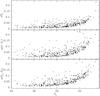 |
Fig. 1 Magnitude and colour photometric errors as a function of T1 for a 30″ circular extraction around NGC 2093. |
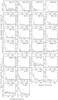 |
Fig. 2 Density profiles for the studied clusters. The horizonal lines represent the adopted background levels. |
Since all the CMDs reveal both cluster and field star characteristics that are more or less superimposed, we should first separate the cluster stars from those belonging to the surrounding fields in order to estimate the cluster fundamental parameters from their CMDs. Both cluster and field stars are, all in all, affected by nearly the same interstellar reddening, which is indeed what causes the overlapping of their main sequences (MSs). This makes the cleaning of the CMDs even more difficult. Then, we carried out a statistical field star cleaning in the cluster CMDs to highlight the cluster features. We selected as reference star fields equal cluster area rings around the cluster centres with internal radii four times those of the respective cluster radii.
Using each annular field CMD, we counted how many stars lie in different magnitude-colour bins with sizes [ΔT1, Δ(C − T1) = (0.2, 0.05), (0.2, 0.1), (0.5, 0.1), and (0.5, 0.2) mag. Then, we subtracted the number of stars counted for each bin of the field [T1, (C − T1)] CMDs from their cluster regions. Thus, we removed those stars closer in magnitude and colour to the ones in the star fields. We obtained, therefore, four different subtracted CMDs for each cluster field. With the aim of comparing the resulting residuals, we applied this filtering procedure by also using the four bin sets shifted by half of their sizes. This method rendered eight tables for each observed cluster field. Each of them contains the stars that have not been subtracted located within the cluster region, since we eliminated those matching the spatial density, magnitude, and colour distributions of the selected star fields.
We finally adopted as the cluster CMDs those generated with stars appearing in the corresponding eight tables. In order to illustrate the statistical cleaning procedure, Fig. 3 shows the CMDs for stars distributed within the cluster radii and the resulting cleaned cluster stars. The resulting CMDs do contain not only cluster stars but also the unavoidable residuals. However, when comparing field and cleaned cluster CMDs, differences in stellar composition become noticeable; for example, it is possible to distinguish the main sequence turnoffs (MSTOs) and red clumps (RCs) in all the clusters, as well as MSs extended from one up to four magnitudes downwards. We recall that the identified clusters are small angular size objects projected or immersed in dense star fields, so that the crowding effect could be responsible for the limited magnitude reached in some cases.
Fundamental parameters of LMC clusters.
We computed E(B − V) colour excesses by interpolating the extinction maps of Burstein & Heiles (1982) using a grid of (l, b) values, with steps of Δ(l, b) = (0.01°, 0.01°) covering the observed fields. We obtained between 80 and 100 colour excesses per cluster field. Then, we built histograms and calculated their centres and FWHMs. Since the FWHMs values turned out to be considerably low, we assumed that the interstellar absorption is uniform across the cluster fields. Table 3 lists the derived E(B − V) colour excesses. As for the cluster distance moduli, Subramanian & Subramanian (2009) find that the average depth for the LMC disk is 3.44 ± 1.16 kpc, so that the difference in apparent distance modulus – clusters could be placed in front of, or behind the LMC – could be as large as Δ((m − M)0) ~ 0.3 mag, if a value of 50 kpc is adopted for the mean LMC distance (Subramanian & Subramanian 2010). Since a difference of 0.10 in log(t) (the difference between two close isochrones in the Girardi et al. 2002, models used here) implies a difference of ~0.5 mag in T1, we decided to adopt the value of the LMC distance modulus (m − M)0 = 18.50 ± 0.10 reported by Saha et al. (2010) for all the clusters.
To estimate the ages of the clusters we used the isochrones of Girardi et al. (2002), including core overshooting, for Z = 0.008 ( [Fe/H = −0.4 dex, Piatti et al. 2009). We then selected a set of isochrones and superimposed them on the cluster CMDs, once they were properly shifted by the corresponding E(B − V) colour excesses and by the LMC distance modulus using the equations E(C − T1) = 1.97E(B − V) and MT1 = T1 + 0.58E(B − V) − (V − MV) (Geisler & Sarajedini 1999). In the matching procedure we employed seven different isochrones, ranging from slightly younger than the derived cluster age to slightly older. Finally, we adopted as the cluster age the one corresponding to the isochrone that was visually judged as best reproducing the cluster main features, while its error was estimated by taking the isochrones into account that mostly encompass those features. For each cluster CMD (Fig. 3), we plotted the isochrone of the adopted cluster age and two additional isochrones at ± 0.05 or 0.10 in log(t) (see age errors in Table 3). These adjacent isochrones span most of the T1 turnoff range, so that they can be considered to be a measure of the age errors. We recall that Pietrzyński & Udalski (2000, hereafter PU00) and Glatt et al. (2010, hereafter GGK10) have studied some of the present clusters (see Table 3) assuming that they are clusters younger than 1 Gyr. GGK10 showed that the dispersion about the 1:1 agreement with PU00 for 49 clusters in common is σlog (t) = 0.15, so that no zero age offset was needed to apply. Our ages also agree well with those quoted by them (σlog (t) = 0.15 around the 1:1 relationship), although some few differences arise. As they mentioned, this could be due to their limited photometric depth and/or biased field star contamination cleaning.
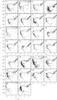 |
Fig. 3 Extracted Washington T1 versus C − T1 CMDs for stars distributed within the cluster radii (small circles), and the cluster cleaned from field contamination (big circles): 1) BSDL 716, 2) BSDL 1024, 3) BSDL 1035, 4) BSDL 2995, 5) H88-26, 6) H88-40, 7) H88-55, 8) H88-188, 9) H88-245, 10) H88-333, 11) HS 38, 12) HS 151, 13) HS 154, 14) KMHK 229, 15) KMHK 506, 16) KMHK 1045, 17) KMHK 1055, 18) LW 469, 19) NGC 2093, 20) SL 154, 21) SL 229, 22) SL 293, 23) SL 300, 24) SL 351, 25) SL 510, and 26) SL 588. The three available isochrones of Girardi et al. (2002) which best resemble the cluster features are overplotted. |
3. Summary
In this study we present, for the first time, CCD Washington photometry of stars in the field of 26 mostly unstudied LMC clusters. CMD cluster features turn out to be identificable when performing annular extractions around their respective centres, once they were cleaned from field star contamination. The clusters turned out to be small angular size objects projected or immersed in dense star fields. We estimated their ages from isochrone fitting, along with the E(B − V) colour excesses, assuming a metallicity of Z = 0.008 ( [Fe/H = −0.4 dex) and an LMC distance modulus of (m − M)0 = 18.50 ± 0.10 mag.
Acknowledgments
I greatly appreciate the comments and suggestions raised by the reviewer, which helped me to improve the manuscript. This research draws upon data distributed by the NOAO Science Archive. NOAO is operated by the Association of Universities for Research in Astronomy (AURA), Inc. under a cooperative agreement with the National Science Foundation. This work was partially supported by the Argentinian institutions CONICET and Agencia Nacional de Promoción Científica y Tecnológica (ANPCyT).
References
- Bica, E., Bonatto, C., Dutra, C. M., & Santos, Jr. J. F. C. 2008, MNRAS, 389, 678 [NASA ADS] [CrossRef] [Google Scholar]
- Burstein, D., & Heiles, C. 1982, AJ, 87, 1165 [NASA ADS] [CrossRef] [Google Scholar]
- de Grijs, R., & Anders, P. 2006, MNRAS, 366, 295 [NASA ADS] [CrossRef] [Google Scholar]
- Geisler, D. 1996, AJ, 111, 480 [NASA ADS] [CrossRef] [Google Scholar]
- Geisler, D., & Sarajedini, A. 1999, AJ, 117, 308 [NASA ADS] [CrossRef] [Google Scholar]
- Girardi, L., Bertelli, G., Bressan, A., et al. 2002, A&A, 391, 195 [NASA ADS] [CrossRef] [EDP Sciences] [Google Scholar]
- Glatt, K., Grebel, E. K., & Koch, A. 2010, A&A, 517, A50 [NASA ADS] [CrossRef] [EDP Sciences] [Google Scholar]
- Harris, J., & Zaritsky, D. 2009, AJ, 138, 1243 [NASA ADS] [CrossRef] [Google Scholar]
- Jannuzi, B. T., Claver, J., & Valdes, F. 2003, The NOAO Deep Wide-Field Survey MOSAIC Data Reductions, http://www.noao.edu/noao/noaodeep/ReductionOpt/frames.html [Google Scholar]
- Maschberger, Th., & Kroupa, P. 2011, MNRAS, 411, 1495 [NASA ADS] [CrossRef] [Google Scholar]
- Pandey, A. K., Sandhu, T. S., Sagar, R., & Battinelli, P. 2010, MNRAS, 403, 1491 [NASA ADS] [CrossRef] [Google Scholar]
- Piatti, A. E. 2011, MNRAS, 418, L40 (P11) [NASA ADS] [CrossRef] [Google Scholar]
- Piatti, A. E., Geisler, D., Sarajedini, A., & Gallart, C. 2009, A&A, 501, 585 [NASA ADS] [CrossRef] [EDP Sciences] [Google Scholar]
- Pietrzyński, G., & Udalski, A. 2000, Acta Astron., 50, 337 [NASA ADS] [Google Scholar]
- Saha, A., Olszewski, E. W., Brondel, B., et al. 2010, AJ, 140, 1719 [NASA ADS] [CrossRef] [Google Scholar]
- Stetson, P. B., Davis, L. E., & Crabtree, D. R. 1990, in CCDs in Astronomy (San Francisco: ASP), ASP Conf. Ser., 8, 289 [Google Scholar]
- Subramanian, S., & Subramanian, A. 2009, A&A, 496, 399 [NASA ADS] [CrossRef] [EDP Sciences] [Google Scholar]
- Subramanian, S., & Subramanian, A. 2010, A&A, 520, A24 [NASA ADS] [CrossRef] [EDP Sciences] [Google Scholar]
All Tables
All Figures
|
Fig. 1 Magnitude and colour photometric errors as a function of T1 for a 30″ circular extraction around NGC 2093. |
| In the text | |
|
Fig. 2 Density profiles for the studied clusters. The horizonal lines represent the adopted background levels. |
| In the text | |
|
Fig. 3 Extracted Washington T1 versus C − T1 CMDs for stars distributed within the cluster radii (small circles), and the cluster cleaned from field contamination (big circles): 1) BSDL 716, 2) BSDL 1024, 3) BSDL 1035, 4) BSDL 2995, 5) H88-26, 6) H88-40, 7) H88-55, 8) H88-188, 9) H88-245, 10) H88-333, 11) HS 38, 12) HS 151, 13) HS 154, 14) KMHK 229, 15) KMHK 506, 16) KMHK 1045, 17) KMHK 1055, 18) LW 469, 19) NGC 2093, 20) SL 154, 21) SL 229, 22) SL 293, 23) SL 300, 24) SL 351, 25) SL 510, and 26) SL 588. The three available isochrones of Girardi et al. (2002) which best resemble the cluster features are overplotted. |
| In the text | |
Current usage metrics show cumulative count of Article Views (full-text article views including HTML views, PDF and ePub downloads, according to the available data) and Abstracts Views on Vision4Press platform.
Data correspond to usage on the plateform after 2015. The current usage metrics is available 48-96 hours after online publication and is updated daily on week days.
Initial download of the metrics may take a while.