| Issue |
A&A
Volume 539, March 2012
|
|
|---|---|---|
| Article Number | A81 | |
| Number of page(s) | 7 | |
| Section | Interstellar and circumstellar matter | |
| DOI | https://doi.org/10.1051/0004-6361/201117528 | |
| Published online | 27 February 2012 | |
Warm gas at 50 AU in the disk around Herbig Be star HD 100546 ⋆
1 Max-Planck-Institut für Astronomie, Königstuhl 17, 69117 Heidelberg, Germany
e-mail: This email address is being protected from spambots. You need JavaScript enabled to view it.
2 Astronomical Institute “Anton Pannekoek” at the University van Amsterdam, The Netherlands
3 ESO, Karl-Schwarzschild-Straße 2, 85748 Garching bei München, Germany
4 Institut für Theoretische Astrophysik, Universität Heidelberg, Albert-Ueberle-Str. 2, 69120 Heidelberg, Germany
5 ISDC Data Centre for Astrophysics & Geneva Observatory, University of Geneva, chemin d’Ecogia 16, 1290 Versoix, Switzerland
6 Universidad Autónoma de Madrid, Cantoblanco, 28049 Madrid, Spain
7 Thüringer Landessternwarte Tautenburg, Sternwarte 5, 07778 Tautenburg, Germany
Received: 20 June 2011
Accepted: 28 November 2011
Abstract
Context. The disk atmosphere is one of the fundamental elements of theoretical models of a protoplanetary disk. However, the direct observation of the warm gas (≫100 K) at large radius of a disk (≫10 AU) is challenging, because the line emission from warm gas in a disk is usually dominated by the emission from an inner disk.
Aims. Our goal is to detect the warm gas in the disk atmosphere well beyond 10 AU from a central star in a nearby disk system of the Herbig Be star HD 100546.
Methods. We measured the excitation temperature of the vibrational transition of CO at incremental radii of the disk from the central star up to 50 AU, using an adaptive optics system combined with the high-resolution infrared spectrograph CRIRES at the VLT.
Results. The observation successfully resolved the line emission with 0.″1 angular resolution, which is 10 AU at the distance of HD 100546. Population diagrams were constructed at each location of the disk, and compared with the models calculated taking into account the optical depth effect in LTE condition. The excitation temperature of CO is 400–500 K or higher at 50 AU away from the star, where the blackbody temperature in equilibrium with the stellar radiation drops as low as 90 K. This is unambiguous evidence of a warm disk atmosphere far away from the central star.
Key words: circumstellar matter / stars: pre-main sequence / protoplanetary disks / stars: individual HD 100546 / stars: variables: T Tauri, Herbig Ae, Be / stars: formation
Based on data collected in the course of CRIRES program [084.C-0605] at the VLT on Cerro Paranal (Chile), which is operated by the European Southern Observatory (ESO).
© ESO, 2012
1. Introduction
A warm disk atmosphere is a natural consequence of a disk externally heated by stellar radiation (e.g. Calvet et al. 1991; Aikawa et al. 2002). Together with a somewhat cooler mid-plane and a disk inner-rim, it is one of the fundamental elements of the current theoretical models on which our understanding of a protoplanetary disk relies (e.g. Dullemond et al. 2001). The emission from warm gas (≫100 K) in a protoplanetary disk has been best observed in the vibrational transitions of CO (e.g. Goto et al. 2006; Brittain et al. 2007; Najita et al. 2007) and other molecules (e.g. Weintraub et al. 2000; Carr et al. 2004). It is hard to estimate the physical properties of the disk atmosphere from this spatially unresolved line emission alone, however, because the emission from the warm gas is dominated by the strong radiation from the hot inner disk closer to the central star (Brittain et al. 2007; van der Plas et al. 2009). Sub-mm spectroscopy does probe the molecules in the outer disk (>100 AU) through the rotational transitions, but mostly cool gas of the temperature 15–30 K (e.g. Dent et al. 2005; Panić et al. 2010). In order to measure the hot gas in the disk atmosphere at radii of 10 to 100 AU, one requires (1) high angular resolution to exclusively observe the faint emission from the outer disk without being affected by the strong emission from the inner disk; (2) a proper spectroscopic probe that is sensitive to the warm disk atmosphere, many of which are in the infrared regime; and (3) the multiple transitions of that spectroscopic probe to measure the gas temperature quantitatively.
The goal of our observation is to measure the rotational excitation temperature of CO fundamental band at 50 AU away from a star, using an adaptive optics system to isolate the emission of the outer disk from that of the inner rim. The nearest Herbig Be star to the solar system, HD 100546 (B9.5Vne; Houk & Cowley 1975), is used as a testbed, because of its close distance (d = 103 pc; van den Ancker 1998) and high luminosity (L∗ = 26 L⊙; Tatulli et al. 2011). HD 100546 is a 10 Myr-old (van den Ancker 1998), flared disk system (Meeus et al. 2001) (Mdisk > 10-3 M⊙; Panić & Hogerheijde 2009) inclined away from the observers by 40°–50° (e.g., Ardila et al. 2007), with two spiral arms seen at 200 AU in the scattered light (Grady et al. 2001, 2005). The dust disk is truncated at 10 AU and inward (Bouwman et al. 2003; Acke & van den Ancker 2006). The gas and the dust at the inner rim are warm, 200 K and 1000 K, respectively, under the direct irradiation of the central star (Bouwman et al. 2003; Brittain et al. 2009). The vibrational transition of CO and H2 have been spatially resolved (Brittain et al. 2009; van der Plas et al. 2009; Carmona et al. 2011), but the disk atmosphere has not been studied in depth, because the emission from the outer disk was not properly separated from that of the inner rim. In this paper, we will follow up these studies, and measure the gas temperature in the disk atmosphere quantitatively.
2. Observations
The observation was carried out with CRIRES (Käufl et al. 2004) at the VLT on 29 and 30 April in 2010 in the open-time program 084.C-0605. The adaptive optics system MACAO (Bonnet et al. 2004) was used to feed nearly diffraction-limited images to the spectrograph using HD 100546 as a wavefront reference. The slit width was 0 2, providing spectra with a velocity resolution of 3 km s-1 (R = 100 000). The spectroscopy covers the wavelength from 4.588 μm to 5.004 μm [R(16)–R(0), P(1)–P(27)] continuously with six grating settings. The spectra were obtained with the observing template CRIRES_spec_obs_SpectroAstrometry. The slit was oriented eight position angles to increase the spatial coverage of the disk. We here used the subset of the data with the slit aligned to the major axis of the disk projected onto the sky (PA = 145°; Ardila et al. 2007), and anti-parallel to it (PA = 325°) to test the consistency of the detected line emissions, and the measurement of the excitation temperature of CO. The telescope was nodded by 10′′ every two exposures to subtract the thermal emission from the sky. The total integration time was 4 minutes for one grating setting. A spectroscopic standard star HR 6556 (A5 III) was observed at close airmass with HD 100546 with the same instrument settings.
3. Data reduction and analysis
The spectral images were pre-processed for subtraction of the dark-current images and flat-fielding, and coadded by cries_spec_jitter recipe1 on the ESO gasgano platform2. Because all line images of v = 2–1 look qualitatively similar, those lines that were not blended with strong telluric absorption lines, or with the other transitions of CO lines, were registered and added to a single line image to increase the signal-to-noise ratio, and to check the spatial extent of the gas emission (Fig. 1). Continuum emission was interpolated from both sides of the line emission, and subtracted. The gas emission of the disk is clearly resolved, showing Keplerian rotation profiles consistently in both line images obtained with slit PA = 145° and 325° with the low-velocity wings extending up to 50 AU. The disk around HD 100546 is known to be brighter at the southwestern side than the northeastern side in the scattered light (Ardila et al. 2007). The asymmetry of the surface brightness has been attributed to the preferential forward scattering of the dust grains in the disk. The rotation of the disk detected in CO v = 2–1 with the southeastern part approaching toward us is consistent with this disk inclination and the counter-clockwise winding of the spiral arms (Grady et al. 2005; Ardila et al. 2007).
One-dimensional spectra were extracted from the spectral images, setting the extraction apertures at the incremental distances from the central star (the positions and the sizes of the extraction apertures are summarized in Table 1). The telluric absorption lines were removed by dividing by the spectra of the spectroscopic standard star after correcting the small mismatches in the wavelengths, the airmass, and the spectral resolutions. The wavelength calibration was performed to match the telluric absorption lines to the atmospheric transmission model calculated by ATRAN (Lord 1992).
Because the transitions to the ground level v = 1–0 were affected by the telluric absorption lines of the same transitions, v = 2–1 lines were used to calculate the column densities of the rotational levels from J = 0 to J = 26 in v = 2 vibrational state to construct the population diagrams. The column density at each J level NJ was calculated for the optically thin limit NJ Aul hν ω = Wνfν, where ω is the solid angle of the emitting area, and fν is the flux density of the continuum emission to convert the equivalent width Wν to the line flux. We were unable to perform the absolute flux calibration of the spectra to measure fν properly because of significant systematic errors from the variable PSF, variable slit transmission, and the variable pixel sampling of the PSF combined together. The factor fν/ω is irrelevant here, though, as long as it changes only slowly with the wavelength, because we are not primarily interested in the absolute column densities, but the relative distribution of NJ to measure the excitation temperature of CO. The line flux of the spectra obtained with adjacent grating settings were scaled so that the lines that were covered by both grating settings have the same line flux on average. The column densities divided by the statistical weights are shown in Fig. 2 after being shifted vertically by an arbitrarily chosen amount for the presentation.
Obviously, the gas is warm (>400 K) out to the longest distance (49 AU) covered by the observations. In order to measure the excitation temperature of CO quantitatively, model population diagrams were calculated based on synthetic line emission spectra, and compared to the observations. The column densities in the upper and lower levels are given by N(u,l) = Nv = (1,2) g(u,l)/Q(u,l) e − E(u,l)/kTex in the LTE condition, where Nv = (1,2) is the total CO column density at v = 1 or 2 state, g is the statistical weight, Q is the partition function, E(u,l) is the energy of the upper or lower level with respect to the rotational ground level, and Tex is the excitation temperature. The line source function of a two-level system was given by Sν = NuAul/(NlBlu − NuBul), and the line emission spectrum was therefore calculated as Iν = Sν (1 − e − τν) with the line opacity  . The line profile φ(ν) was assumed to be a Gaussian function. We performed preliminary runs to fit the observed population diagrams by the models with limited sampling of Tex and NCO, varying the line width of the Gaussian line profile from 2 km s-1 to 30 km s-1. The fitting result in terms of the absolute deviation (
 ) became better up to 6 km s-1 in most of the spectra extracted from different disk locations. In several cases the fitting further improved up to 25 km s-1, but very slightly. For simplicity, we fixed the line width to 6 km s-1, and used the same line profile for the spectra extracted at all disk locations. The equivalent widths of the emission lines were measured with the model spectra and converted to the column densities in the same way as the observed spectra. The energy levels, the line center wavelengths, and Einstein Aul coefficients were taken from Goorvitch (1994). A more detailed discussion on the calculation can be found elsewhere (Goto et al. 2011).
Extraction apertures and excitation temperatures.
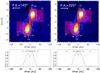 |
Fig. 1 Top: position-velocity diagrams of CO v = 2–1 from HD 100546. All vibrational transitions of CO v = 2–1 in our observational coverage that do not overlap with the deep absorption lines of the terrestrial atmosphere are registered and added. The spectra were recorded with the slit PA = 145° (left) and 325° (right). The spatial axis is in abscissa with the position angles to which the slit was aligned indicated by arrows. The line image obtained with slit PA = 325° is flipped horizontally so that the offset from the central star increases to the right in both of the line images. The continuum emission of the star was interpolated from both sides of the line emission and subtracted. The contours are drawn at every 10% of the peak brightness, except the lowest one which is at 5%. The apertures of the spectral extraction are marked by rectangles. Faint emission is still visible at 50 AU away at low velocity. The sizes and the locations of the extraction apertures are summarized in Table 1. Bottom: spatial profile of the line emission, i.e., the position-velocity diagram shown in the upper panels are crushed along the velocity space. |
The line emission is apparently optically thick with turnovers seen around EJ/k ~ 6500 K. The excitation temperature and the column density are heavily degenerated in these cases. The formal fitting error might underestimate the realistic uncertainty in the temperature measured. We produced contour maps of the absolute deviations between calculated and observed population diagrams on a grid of temperatures (500–2500 K) and column densities (1019–1022 cm-2) (Figs. A.1, A.2). The total extents of the contour in temperature where the absolute deviation increases by 10% of the best fitting value were taken as the uncertainties of the excitation temperature of CO (Fig. 3, Table 1). We lack the measurements of the equivalent widths of high-J levels at 49 AU because of the insufficient signal-to-noise ratio of the spectra (Fig. 2). The upper limit of the excitation temperature is therefore less constrained at the radius than at other locations, but the conclusion (Tex > 400 K) is not affected. Fitting was also performed with the column densities fixed to 1020 cm-2 to give an independent estimate of how the result is affected by this degeneracy. The resulting excitation temperatures do not differ by more than the extent of the errors estimated above except at −49 AU with PA = 145°.
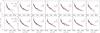 |
Fig. 2 Population diagrams of CO v = 2–1 based on the spectra extracted at the incremental distances from the central star. The upper and the lower panels are from the spectra recorded with the slit PA = 145° and 325°. Open circles and filled triangles are for R- and P-branches, respectively. The column densities divided by the statistical weights are vertically shifted by arbitrarily amount for the presentation. The uncertainty of the individual column density is on the order of the dispersions of the data points. The red lines are the best-fit LTE model population diagrams assuming Gaussian line width of 6 km s-1. The blue lines are the same but the column density of CO is fixed to NCO = 1020 cm-2. |
4. Discussion
The rotational excitation temperature of CO is between 400 K and 1100 K at all locations on the disk where the spectra were extracted. There might be a hint of the cooling of the gas down to 400–600 K with the distance from the central star, but this is not unambiguous. The measurements are consistent in the data with PA = 145° and 325°, except at the edge of the disk at ± 49 AU, and the inner disk at + 9 AU from the star. The latter might be picking up the emission from the hot inner rim exclusively. Although the observation was made with high angular resolution, the line emission from different radii of the disk overlap up to 22 AU, because the emission from the inner rim is by far stronger than that from the disk behind (the spatial profiles of the line emission are shown in the lower panels in Fig. 1). However, as is seen in the locations of the extraction apertures overlaid with the line images (Fig. 1), the spatial resolution is sufficiently high that little blending with the emission from the inner disk is expected at 50 AU and beyond. The excitation temperature is still hotter than 400 K at 49 AU, where the blackbody equilibrium temperature with the stellar radiation [ ; σ, L∗, d are the Stefan-Boltzmann constant, the luminosity of the star, and the distance from the star to the particle] drops as low as 90 K.
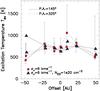 |
Fig. 3 Radial profile of the rotational excitation temperature of CO v = 2–1 in the disk atmosphere of HD 100546 system. Data points are horizontally shifted slightly for clarity. The excitation temperatures are measured from the population diagrams presented in Fig. 2. The red squares are for an LTE model with fixed line width of 6 km s-1. The line emissions are optically thick, therefore the column density and the excitation temperature are highly degenerated. The error bars are given not by the fitting error in Fig. 2, but by the total extent of the contour in temperature in the absolute deviation plots in Figs. A.1 and A.2, where the absolute deviation becomes worse by 10% of the best fitting values. The blue triangles are from the fitting of the population diagrams, but with the column density of CO fixed to NCO = 1020 cm-2. |
Although the presence of this warm gas is exactly what the disk model predicts (Kamp & Dullemond 2004; Jonkheid et al. 2004), this is the first time that the temperature of the disk atmosphere is directly measured beyond the disk inner rim by a high angular resolution observation that spatially resolved the disk. The range of the excitation temperature nicely overlaps with 300–800 K of the pure rotational lines of CO at high-J (14 ≤ J ≤ 30) measured in the recent spectroscopy of the same object by Herschel/PACS (Sturm et al. 2010). Thi et al. (2011) also detected CH+J = 5–4, 6–5, 3–2 by the same instrument, and derived a rotational excitation temperature 323 K. It is inferred that these observations are likely looking at the gas in a similar location of the disk as the present study. The model presented by Thi et al. (2011), which takes into account the specific disk geometry of HD 100546 constrained by the spectral energy distribution (Benisty et al. 2010), also shows a warm layer of the gas at 50 AU of the disk.
A mechanism that likely vibrationally excites CO to v = 2 level is the ultraviolet pumping (Krotkov et al. 1980), because the vibrational temperature (Tvib = 6600 ± 700 K; van der Plas 2010) is much hotter than the rotational excitation temperature (Brittain et al. 2009). The rotational levels are much faster to thermalize through the collisions with the molecular/atomic hydrogen and therefore should represent the ambient gas temperature better. It is in principle possible to account for the extended line emission not by the emission arising on the site, but by the scattered line emission, where CO is excited to v = 2 level in the vicinity of the central star, and the line emission emerging from the hot inner disk is simply reflected into the line of sights to observers by the dust grains at 50 AU. We discarded the scattered line emission, because the line images in Fig. 1 clearly show the Keplerian profiles, which indicate that the line center velocity at 50 AU is closer to the system velocity than that of the gas orbiting closer to the central star.
The observed excitation temperature agrees with that of Jonkheid et al. (2007), who calculated the chemistry and the temperature structure of a disk around a Herbig Ae star without the a priori assumption that the gas is physically coupled to the dust. The calculations were performed for the disk mass from 10-1 to 10-4 M⊙ to simulate the dissipation of a disk, and with and without the dust settling, i.e., the mass ratio of the dust and the gas in the upper layer gradually reduced from 0.01 to 10-5. The gas temperature in the upper layer is clearly higher in cases without dust settling, because the gas is primarily heated by the photoelectric effect of the dust grains. The gas is hotter than 300 K in the disk atmosphere at the distance of 50 AU from the disk surface to the significant depth toward the mid-plane for all the disk models calculated without dust settling, which is comfortably matched with the excitation temperature we found; while the gas temperature with dust settling is everywhere less than 100 K. That the disk atmosphere is well mixed with the dust grains is also consistent with the classification of the source as Ia by Meeus et al. (2001) with spatially resolved (Habart et al. 2006), rich emission features of PAHs (Acke et al. 2010), and the thermal continuum emission extended up to 14, or 145 AU, in the mid-infrared (Mulders et al. 2011).
CRIRES Pipeline User Manual VLT-MAN-ESO-19500-4406.
Acknowledgments
We appreciate the constructive criticisms of the anonymous referee that improved the manuscript. We thank all the staff and crew of the VLT for their valuable assistance in obtaining the data. We appreciate the hospitality of the Chilean community that made the research presented here possible.
References
- Acke, B., & van den Ancker, M. E. 2006, A&A, 449, 267 [NASA ADS] [CrossRef] [EDP Sciences] [Google Scholar]
- Acke, B., Bouwman, J., Juhász, A., et al. 2010, ApJ, 718, 558 [NASA ADS] [CrossRef] [Google Scholar]
- Aikawa, Y., van Zadelhoff, G. J., van Dishoeck, E. F., & Herbst, E. 2002, A&A, 386, 622 [NASA ADS] [CrossRef] [EDP Sciences] [Google Scholar]
- Ardila, D. R., Golimowski, D. A., Krist, J. E., et al. 2007, ApJ, 665, 512 [NASA ADS] [CrossRef] [Google Scholar]
- Benisty, M., Tatulli, E., Ménard, F., & Swain, M. R. 2010, A&A, 511, A75 [NASA ADS] [CrossRef] [EDP Sciences] [Google Scholar]
- Bonnet, H., Abuter, R., Baker, A., et al. 2004, The ESO Messenger, 117, 17 [Google Scholar]
- Bouwman, J., de Koter, A., & Dominik, C. 2003, A&A, 410, 577 [NASA ADS] [CrossRef] [EDP Sciences] [Google Scholar]
- Brittain, S. D., Simon, T., Najita, J. R., & Rettig, T. W. 2007, ApJ, 659, 685 [NASA ADS] [CrossRef] [Google Scholar]
- Brittain, S. D., Najita, J. R., & Carr, J. S. 2009, ApJ, 702, 858 [NASA ADS] [Google Scholar]
- Calvet, N., Patino, A., Magris, G. C., & D’Alessio, P. 1991, ApJ, 380, 617 [NASA ADS] [CrossRef] [Google Scholar]
- Carmona, A., van der Plas, G., van den Ancker, M. E., et al. 2011, A&A, 533, A39 [NASA ADS] [CrossRef] [EDP Sciences] [Google Scholar]
- Carr, J. S., Tokunaga, A. T., & Najita, J. 2004, ApJ, 603, 213 [NASA ADS] [CrossRef] [Google Scholar]
- Dent, W. R. F., Greaves, J. S., & Coulson, I. M. 2005, MNRAS, 359, 663 [NASA ADS] [CrossRef] [Google Scholar]
- Dullemond, C. P., Dominik, C., & Natta, A. 2001, ApJ, 560, 957 [NASA ADS] [CrossRef] [Google Scholar]
- Goorvitch, D. 1994, ApJS, 95, 535 [NASA ADS] [CrossRef] [Google Scholar]
- Goto, M., Regály, Zs., Dullemond, C. P., et al. 2011, ApJ, 728, 5 [NASA ADS] [CrossRef] [Google Scholar]
- Goto, M., Usuda, T., Dullemond, C. P., et al. 2006, ApJ, 652, 758 [NASA ADS] [CrossRef] [Google Scholar]
- Grady, C. A., Polomski, E. F., Henning, T., et al. 2001, AJ, 122, 3396 [NASA ADS] [CrossRef] [Google Scholar]
- Grady, C. A., Woodgate, B., Heap, S. R., et al. 2005, ApJ, 620, 470 [Google Scholar]
- Habart, E., Natta, A. A., Testi, L., & Carbillet, M. 2006, A&A, 449, 1067 [NASA ADS] [CrossRef] [EDP Sciences] [Google Scholar]
- Houk, N., & Cowley, A. P. 1975, Michigan Spectral Survey (Univ. Michigan Press), 1 [Google Scholar]
- Jonkheid, B., Faas, F. G. A., van Zadelhoff, G., & van Dishoeck, E. F. 2004, A&A, 428, 511 [NASA ADS] [CrossRef] [EDP Sciences] [Google Scholar]
- Jonkheid, B., Dullemond, C. P., Hogerheijde, M. R., & van Dishoeck, E. F. 2007, A&A, 463, 203 [NASA ADS] [CrossRef] [EDP Sciences] [Google Scholar]
- Kamp, I., & Dullemond, C. P. 2004, ApJ, 615, 991 [NASA ADS] [CrossRef] [Google Scholar]
- Käufl, H. U., Ballester, P., Biereichel, P., et al. 2004, Proc. SPIE, 5492, 1218 [CrossRef] [Google Scholar]
- Krotkov, R., Wang, D., & Scoville, N. Z. 1980, ApJ, 240, 940 [NASA ADS] [CrossRef] [Google Scholar]
- Lord, S. D. 1992, A New Software Tool for Computing Earth’s Atmosphere Transmissions of Near- and Far-Infrared Radiation, NASA Technical Memoir 103957 (Moffett Field, CA: NASA Ames Research Center) [Google Scholar]
- Meeus, G., Waters, L. B. F. M., Bouwman, J., et al. 2001, A&A, 365, 476 [NASA ADS] [CrossRef] [EDP Sciences] [Google Scholar]
- Mulders, G. D., Waters, L. B. F. M., Dominik, C., et al. 2011, A&A, 531, A93 [NASA ADS] [CrossRef] [EDP Sciences] [Google Scholar]
- Najita, J. R., Carr, J. S., Glassgold, A. E., & Valenti, J. A. 2007, in Protostars and Planets V, 507 [Google Scholar]
- Panić, O., & Hogerheijde, M. R. 2009, A&A, 508, 707 [NASA ADS] [CrossRef] [EDP Sciences] [Google Scholar]
- Panić, O., van Dishoeck, E. F., Hogerheijde, M. R., et al. 2010, A&A, 519, A110 [NASA ADS] [CrossRef] [EDP Sciences] [Google Scholar]
- Sturm, B., Bouwman, J., Henning, T., et al. 2010, A&A, 518, L129 [NASA ADS] [CrossRef] [EDP Sciences] [Google Scholar]
- Tatulli, E., Benisty, M., Ménard, F., et al. 2011, A&A, 531, A1 [NASA ADS] [CrossRef] [EDP Sciences] [Google Scholar]
- Thi, W. F., Ménard, F., Meeus, G., et al. 2011, A&A, 530, L2 [NASA ADS] [CrossRef] [EDP Sciences] [Google Scholar]
- van der Plas, G. 2010, Ph.D Thesis, University of Amsterdam [Google Scholar]
- van der Plas, G., van den Ancker, M. E., Acke, B., et al. 2009, A&A, 500, 1137 [NASA ADS] [CrossRef] [EDP Sciences] [Google Scholar]
- van den Ancker, M. E., de Winter, D., Tjin, A., & Djie, H. R. E. 1998, A&A, 330, 145 [NASA ADS] [Google Scholar]
- Weintraub, D. A., Kastner, J. H., & Bary, J. S. 2000, ApJ, 541, 767 [NASA ADS] [CrossRef] [Google Scholar]
Appendix A: Measurement of rotational excitation temperature
Here we provide the contour maps of the absolute deviations between calculated and observed population diagrams that we used to estimate the uncertainty of the excitation temperature of CO. The extents of the contour in the temperature where the absolute deviation increases by 10% of the best fitting value were taken as the error of Tex.
 |
Fig. A.1 Contour maps of the absolute deviations between the calculated and observed population diagrams. The observed population diagrams are based on the data obtained with the slit PA = 145°. Tex and NCO that give the minimum absolute deviations are marked by crosses. The contours are drawn at every 10% increase of the absolute deviation from its minimum value. |
All Tables
All Figures
|
Fig. 1 Top: position-velocity diagrams of CO v = 2–1 from HD 100546. All vibrational transitions of CO v = 2–1 in our observational coverage that do not overlap with the deep absorption lines of the terrestrial atmosphere are registered and added. The spectra were recorded with the slit PA = 145° (left) and 325° (right). The spatial axis is in abscissa with the position angles to which the slit was aligned indicated by arrows. The line image obtained with slit PA = 325° is flipped horizontally so that the offset from the central star increases to the right in both of the line images. The continuum emission of the star was interpolated from both sides of the line emission and subtracted. The contours are drawn at every 10% of the peak brightness, except the lowest one which is at 5%. The apertures of the spectral extraction are marked by rectangles. Faint emission is still visible at 50 AU away at low velocity. The sizes and the locations of the extraction apertures are summarized in Table 1. Bottom: spatial profile of the line emission, i.e., the position-velocity diagram shown in the upper panels are crushed along the velocity space. |
| In the text | |
|
Fig. 2 Population diagrams of CO v = 2–1 based on the spectra extracted at the incremental distances from the central star. The upper and the lower panels are from the spectra recorded with the slit PA = 145° and 325°. Open circles and filled triangles are for R- and P-branches, respectively. The column densities divided by the statistical weights are vertically shifted by arbitrarily amount for the presentation. The uncertainty of the individual column density is on the order of the dispersions of the data points. The red lines are the best-fit LTE model population diagrams assuming Gaussian line width of 6 km s-1. The blue lines are the same but the column density of CO is fixed to NCO = 1020 cm-2. |
| In the text | |
|
Fig. 3 Radial profile of the rotational excitation temperature of CO v = 2–1 in the disk atmosphere of HD 100546 system. Data points are horizontally shifted slightly for clarity. The excitation temperatures are measured from the population diagrams presented in Fig. 2. The red squares are for an LTE model with fixed line width of 6 km s-1. The line emissions are optically thick, therefore the column density and the excitation temperature are highly degenerated. The error bars are given not by the fitting error in Fig. 2, but by the total extent of the contour in temperature in the absolute deviation plots in Figs. A.1 and A.2, where the absolute deviation becomes worse by 10% of the best fitting values. The blue triangles are from the fitting of the population diagrams, but with the column density of CO fixed to NCO = 1020 cm-2. |
| In the text | |
|
Fig. A.1 Contour maps of the absolute deviations between the calculated and observed population diagrams. The observed population diagrams are based on the data obtained with the slit PA = 145°. Tex and NCO that give the minimum absolute deviations are marked by crosses. The contours are drawn at every 10% increase of the absolute deviation from its minimum value. |
| In the text | |
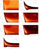 |
Fig. A.2 Same as Fig. A.1, but for the data obtained with the slit PA = 325°. |
| In the text | |
Current usage metrics show cumulative count of Article Views (full-text article views including HTML views, PDF and ePub downloads, according to the available data) and Abstracts Views on Vision4Press platform.
Data correspond to usage on the plateform after 2015. The current usage metrics is available 48-96 hours after online publication and is updated daily on week days.
Initial download of the metrics may take a while.