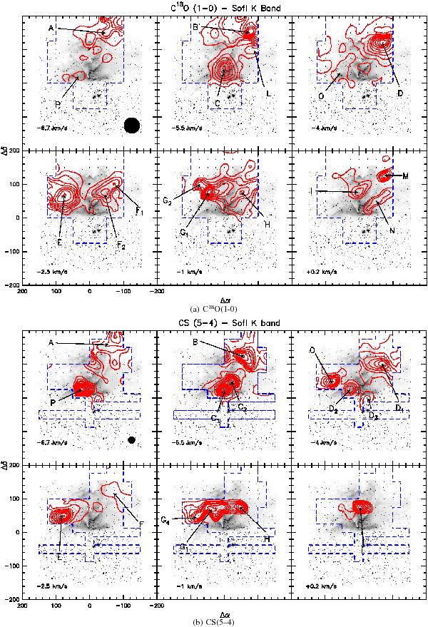
a) Integrated emission of C¹⁸O(1–0) superimposed on the K_s image. Each plot corresponds to a different V_LSR. The V_LSR of the clumps is indicated in the respective panel. The dashed (blue) lines indicate the observed area. The (red) contours show the integral under Gaussian components fitted to the line profiles. The beam of the transition is shown in the first panel. The first contour in each panel is the 3σ level. The integrated emission levels (in units of K km s^-1) are (lowest (step) highest): ( − 6.7 km s^-1) 0.17 (0.3) 2.27; (–5.5 km s^-1, C) 0.19 (0.3) 1.99; ( − 5.5 km s^-1, B) 0.20 (0.5) 4.70; ( − 4.0 km s^-1) 0.18 (0.7) 6.48; ( − 2.5 km s^-1) 0.19 (0.3) 2.89; ( − 1.0 km s^-1) 0.18 (0.2) 1.78; ( + 0.2 km s^-1) 0.15 (0.1) 0.65. b) As a), but for CS(5–4). The integrated emission levels (in units of K km s^-1) are (lowest (step) highest): ( − 6.7 km s^-1) 0.19 (0.3) 2.59; ( − 5.5 km s^-1, C) 0.20 (1.0) 10.20; ( − 5.5 km s^-1, B) 0.19 (0.5) 3.69; ( − 4.0 km s^-1) 0.19 (0.7) 4.39; ( − 2.5 km s^-1) 0.18 (1.0) 8.18; ( − 1.0 km s^-1) 0.17 (0.2) 1.37; ( + 0.2 km s^-1) 0.14 (0.1) 0.74. Note that names of the clumps do not correspond to those used in Massi et al. (1997).