| Issue |
A&A
Volume 537, January 2012
|
|
|---|---|---|
| Article Number | L3 | |
| Number of page(s) | 4 | |
| Section | Letters | |
| DOI | https://doi.org/10.1051/0004-6361/201118084 | |
| Published online | 04 January 2012 | |
Orbital migration induced by anisotropic evaporation
Can hot Jupiters form hot Neptunes?
1 Centro de Astrofísica da Universidade do Porto, Rua das Estrelas, 4150-762 Porto, Portugal
e-mail: This email address is being protected from spambots. You need JavaScript enabled to view it.
2 ASD, IMCCE-CNRS UMR8028, Observatoire de Paris, UPMC, 77 avenue Denfert-Rochereau, 75014 Paris, France
3 Department of Physics, I3N, University of Aveiro, Campus Universitário de Santiago, 3810-193 Aveiro, Portugal
4 Departamento de Física e Astronomia, Faculdade de Ciências, Universidade do Porto, Portugal
Received: 13 September 2011
Accepted: 2 December 2011
Abstract
Short-period planets are subject to intense energetic irradiations from their stars. It has been shown that this can lead to significant atmospheric mass loss and can create lower mass planets. Here, we analyse whether the evaporation mechanism can affect the orbit of planets. The orbital evolution of a planet undergoing evaporation is derived analytically in a very general way. Analytical results are then compared with the period distribution of two classes of inner exoplanets: Jupiter-mass planets and Neptune-mass planets. These two populations have very distinct period distributions, with a probability lower than 10-4 that they were derived from the same parent distribution. We show that mass ejection can generate significant migration with an increase in orbital period that matches the difference in distribution of the two populations very well. This would happen if the evaporation emanates from above the hottest region of planet surface. Thus, migration induced by evaporation is an important mechanism that cannot be neglected.
Key words: planets and satellites: formation / planets and satellites: dynamical evolution and stability / planet-star interactions
© ESO, 2012
1. Introduction
Different scenarios have been proposed to explain the formation of hot Neptunes and super-Earths: migration in a protoplanetary disk (Mordasini et al. 2009), in situ formation by accretion of planetesimals (Brunini & Cionco 2005), embryo formation in a compact multiplanetary system and subsequent migration through scattering (Ida & Lin 2010), tidal downsizing of giant planet embryo (Nayakshin 2010, 2011), or partial evaporation of more massive planets (Baraffe et al. 2004; Lecavelier Des Etangs 2007; Valencia et al. 2010). Here, we focus on the evaporation hypothesis with a particular attention to semi-major axis evolution. Indeed, among the shortest period exoplanets, those closer to their star tend to be more massive than the outer ones (Mazeh et al. 2005; Southworth et al. 2007; Davis & Wheatley 2009; Benítez-Llambay et al. 2011). This has been attributed either to a combined effect of tidal interactions and migration in the protoplanetary disk (Benítez-Llambay et al. 2011) or to the fact that low-mass close-in planets cannot survive catastrophic evaporation (Davis & Wheatley 2009).
While isotropic planetary evaporation generates almost neglectable migration, anisotropic ejection of matter can lead to a substantial increase in the semi-major axis. This effect is similar to anisotropic thermal radiation (Fabrycky 2008). For hot gazeous planets, two different mechanisms have been proposed to explain atmospheric escapes, i.e. how particles reach the Roche lobe (Hill) radius of their planet. On the one hand, this may come from a thermal inflation of the planet. Particles of the upper atmosphere are assumed to follow Maxwellian velocity distribution, and those with the highest speed escape (Gu et al. 2003; Lecavelier des Etangs et al. 2004). In that case, the evaporation is directed mainly towards the L1 Lagrangian point located between the star and the planet (Gu et al. 2003). On the other hand, the escape may be driven by vertical winds on the planet’s dayside (Yelle 2004; García Muñoz 2007; Murray-Clay et al. 2009). This situation is more complex and 3D hydrodynamical simulations are required to get the geometry of ejection. Nevertheless, winds are likely to be anisotropic.
Atmospheric circulation models predict the existence of a jet that displaces the hottest region of hot Jupiters from the substellar point, along the equator (Showman & Guillot 2002). More recent models agree that the jet is a common feature of circulation models and that it is confined to latitudes between –30° and 30° with a displacement from the substellar point usually eastward, by 10–60° of longitude. Its value depends on the strength of the imposed stellar heating and other factors such as the radiative timescale and drag time constant (Showman & Polvani 2011). These predictions are corroborated by the observed surface temperature distribution of HD 189733b (Knutson et al. 2007).
Although there is evidence of a displacement of the hottest region with respect to the substellar point on the planet surface, the dynamics of exobase are poorly known. Strictly speaking, it is thus not possible to establish in which direction and how mass is ejected by evaporation. Hereafter, to get estimates of the migration induced by evaporation, we take the results mentioned above concerning planetary surface as representative of the exobase structure.
This letter is organized as follows. In Sect. 2, we derive a very general expression of the orbital evolution of a planet undergoing evaporation. In Sect. 3, we compare the distribution of two classes of close-in planets: Jupiter and Neptune-like ones. The statistical analysis is then used, in Sect. 4, to constrain the geometry of evaporation assuming that hot Neptunes are partially evaporated hot Jupiters. This geometry is also compared with the predictions of atmospheric models. The conclusion is presented in Sect. 5.
2. Orbital evolution with evaporation
Two-body problems in which one of the component loses mass should be solved with care. Several misunderstandings have already been found in the literature (Plastino & Muzzio 1992), since the equations of motion are not the same when the ejection is isotropic or not. Here, we consider a simple model of evaporation that is well suited to both isotropic and anisotropic mass loss.
We define a planet of mass m(t) orbiting a star with mass m⋆. The orbit is characterized by a radius vector r, an orbital velocity  , a semi-major axis a, an eccentricity e, an orbital angular momentum ℓ = r × v, and a period P = 2π/n, where n is the mean motion defined by G(m + m⋆) = n2a3, and G is the gravitational constant. Then, vp and v⋆ are respectively the velocity of the planet and of the star in a fixed reference frame. The orbital velocity is then v = vp − v⋆. For any vector w, we denote w = ∥w∥ as its norm, and
  its unit vector. The frame
  , where
  and
and  , is used to defined the geometry of the mass ejection, which is given by two parameters: the angle θ between the star and the direction of mass ejection, and the aperture ϕ of the stream (see Fig. 1). In particular, the evaporation is completely focused in one direction when ϕ = 0°, and becomes isotropic when ϕ = 180°. We denote
 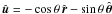 as the average direction of the stream.
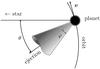 |
Fig. 1 Geometry of evaporation. |
Let Ves be the ejection speed of atmospheric particles with respect to the planet’s barycenter, then Ves can vary between 10 and 20 km s-1 for a planet orbiting a main-sequence star and a T Tauri star, respectively (Murray-Clay et al. 2009). The mean velocity V of the stream is  , where
 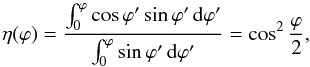 (1)and the equations of motion are
 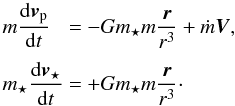 (2)We then assume that the mass-loss rate, ṁ(t), scales linearly with the energy received by the planet from the stellar XEUV emission. It should be stressed that this has no effect on the semi-major axis. Another scaling would modify the eccentricity evolution only slightly. The mass-loss rate is thus inversely proportional to the square of the distance
 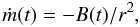 (3)where B(t) is any slowly varying function accounting for the time evolution of the stellar luminosity. From (2), (3), and the expression of V, one gets
  (4)where κ(t) = η(ϕ)B(t)Ves/m(t) and μ(t) = G(m(t) + m⋆) − κ(t)cosθ. Even in the extreme case with a mass-loss rate of ṁ = −1015 g s-1 and an ejection speed of Ves = 100 km s-1, for a hot Jupiter at 0.05 AU, κ/(Gm) remains lower than 2 × 10⁻⁸. In the following, we thus simply use μ(t) = G(m(t) + m⋆).
From the definition of the semi-major axis 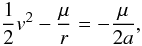 (5)and the expression of the Laplace-Runge-Lenz vector e
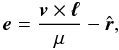 (6)the equation of motion (4) leads to
 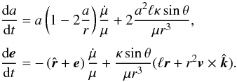 (7)The first terms of the right-hand sides of Eq. (7) are only due to the mass decrease. They do not depend on the geometry and remain unchanged even for isotropic evaporation. On the other hand, the last terms of Eq. (7) vanish for isotropic (κ = 0) or radial (sinθ = 0) mass ejection. The long-term evolution of the orbital parameters is obtained by averaging (7) over the mean anomaly M keeping μ(t), κ(t), and
  constant (e.g. Boué & Laskar 2009). The results are
 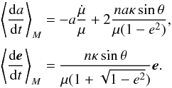 (8)In the following, we consider the simplest case where the orbit is circular. Equation (8) shows that such orbits remain circular over the whole evolution. Replacing B(t) (see Eq. (3)) by − a2ṁ(t) in the expression of κ(t) and using v = na and μ(t) = G(m(t) + m⋆), the secular evolution of the semi-major axis becomes
 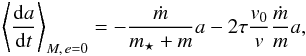 (9)where v0 = v(t = 0) is the initial orbital velocity, and τ is a dimensionless parameter that controls the efficiency of the migration. We thus refer to this parameter as the “migration efficiency”. Its expression is
 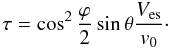 (10)For isotropic evaporation (ϕ = 180°) or radial ejection (θ = 0°), the migration efficiency vanishes. In that case, the product a(m⋆ + m) of the semi-major axis with the total mass of the system remains constant (Hadjidemetriou 1963). Thus, even if a Jupiter-mass planet orbiting a Sun-like star loses all its mass, the semi-major axis increases only by a factor MJup/M⊙ = 0.1%. The term aṁ/(m⋆ + m) in Eq. (9) will thus be neglected in the following.
For arbitrary migration efficiency, the solution of Eq. (9) is a(t) = a0[1 + τln(m(t)/m0)]-2. For convenience, we provide an equivalent relation, with orbital period instead of semi-major axis, deduced from Kepler’s third law 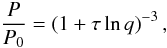 (11)where q = m/m0 is the fraction of mass remaining in the planet. The expression (11) is independent of time, and holds for any mass-loss rate evolutions. The only requirement concerns the efficiency of evaporation. Here, we assume that the evaporation process is strong enough to decrease the mass of a planet from m0 to m.
Using a typical ejection speed Ves = 15 km s-1 and an initial orbital velocity v0 = 145 km s-1 corresponding to a three-day orbit, the order of magnitude of the migration efficiency given by (10) is τ ~ Ves/v0 = 0.1. With this value, if a Jupiter-mass planet is transformed into a Neptune-mass planet by evaporation (q = 0.05), the increase in its orbital period deduced from (11) is P/P0 = 1.5. For comparison, the ratio of the median periods of Jupiter-like planets and Neptune-like planets (see Sect. 3) is 4.9/3.4 = 1.4.
3. Observed period distributions
From the more than 700 exoplanets discovered to date, 204 have orbital periods shorter than ten days and mass lower than 5 MJup1. One can group these planets into two classes: Neptune-mass planets and lower (m < 2 MNep or 2 × 0.054 MJup), and Jupiter-mass planets (m > MSat or 0.3 MJup). The first group contains 37 planets, from which we removed four pairs belonging to the same system2, while the second contains 151. Both correspond to 92% of the short-period planets considered. The two populations are characterized by very distinct period distributions: the Neptunes have a median period of 4.9 days, an average period of 5.3 days, and a standard deviation of 2.6 days, while for the Jupiters the same quantities are of 3.4, 3.5, and 1.6 days, respectively. A Kolmogorov-Smirnov test shows that the cumulative distribution functions (CDF) of the two distributions are significantly different, with the probability that they were derived from the same parent distribution of 3.8 × 10⁻⁵ (see Fig. 2).
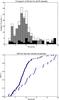 |
Fig. 2 a) Distribution of orbital periods for all planets with m < 5 MJup in white, Jupiters in grey, and Neptunes in black. b) CDFs with their best fit by a log-normal distribution. Jupiters are represented by triangles and Neptunes by circles. |
It is important to keep in mind that the interpretation of these results is conditioned by different factors that warrant discussion. Firstly, the fitted parameters depend on the limits defined for the planetary classes. However, the general properties of the distributions are kept for a wide range of parameters, and the results are expected to be resistant to changes in these parameters. More important is that the observational bias imprinted on the sample by radial-velocity detections, which depends on mass and period, is different for the two classes of planets. Since the amplitude of a signal, hence its detectability, is proportional to mP−1/3, heavier and closer planets are detected more easily than lighter, far away planets. For this reason, the difference in median or average period values is expected to increase for the real unbiased population, showing that the difference in values we found here is not a detection effect but rather an underestimation of the real one. In either case, the reflex motion induced by a Neptune on a ten-day orbit on a one-solar-mass star is 5 m s-1, significantly above the precision of state-of-the-art spectrographs (e.g. HARPS) (Mayor & Udry 2008). As a consequence, we expect the detections reported to date to be representative of the true population.
4. Constraints and comparison with atmospheric models
Here, we derive the distribution of the migration efficiency τ assuming that the hot Neptune and the hot Jupiter populations correspond to the same planets at different degrees of evaporation. This provides constraints on the geometry of evaporation, which are then compared with the results of atmospheric models. That analysis relies on the possibility that hot Jupiters can lose 95% of their mass by evaporation. Although additional work is required, we expect this to happen at the early age of a planet’s history, when stellar emission is strong (Ribas et al. 2005) and planet density is low (e.g. Mordasini et al. 2010). Indeed, these two conditions lead to important mass loss (Erkaev et al. 2007).
To simplify the study and to derive analytical expressions, we approximate the CDFs of the two populations by log-normal distributions 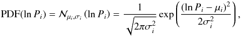 (12)where i ∈ {Jup,Nep}, and Pi is expressed in days.
  is the normal distribution. The best fits give (μJup = 1.19,σJup = 0.39) for Jupiter-like planets and (μNep = 1.62,σNep = 0.57) for Neptune-like planets. Assuming that the migration represented by ΔlnP = lnPNep − lnPJup is independent of PJup and PNep, the law of total probability implies that ΔlnP follows a normal distribution with mean μΔ = μNep − μJup and standard deviation
  . Then, a change of variable from ΔlnP to τ Eq. (11) gives
 ![Mathematical equation: \begin{equation} \PDF(\tau) = -\frac{3 \ln q}{1+\tau \ln q} {\cal N}_{\mu_\Delta, \sigma_\Delta}\left[-3 \ln\left( 1 + \tau \ln q\right)\right] . \label{eq.pdf} \end{equation}](/articles/aa/full_html/2012/01/aa18084-11/aa18084-11-eq98.png) (13)The PDF (13) is plotted in Fig. 3a for q = 0.03, which is the ratio of the geometric mean of the masses of the two planet populations. Using a typical ejection speed Ves = 15 km s-1 and the typical initial orbital velocity v0 = 145 km s-1, the PDF of τ expressed as a function of (θ,ϕ) constrains the geometry of mass ejection (see Fig. 3b).
(13)The PDF (13) is plotted in Fig. 3a for q = 0.03, which is the ratio of the geometric mean of the masses of the two planet populations. Using a typical ejection speed Ves = 15 km s-1 and the typical initial orbital velocity v0 = 145 km s-1, the PDF of τ expressed as a function of (θ,ϕ) constrains the geometry of mass ejection (see Fig. 3b).
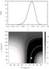 |
Fig. 3 PDF of the migration efficiency τ as a function of τa) or as a function of the angles θ and ϕ (b). In b), the solid line corresponds to the maximum likelihood, the dashed lines delineates the one-sigma confidence region, and the dotted line the two-sigma region. The small circle, at longitude 30° and aperture 30°, shows the approximate location of the hottest region of HD 189733b (Knutson et al. 2007). |
In particular, if considering an aperture ϕ lower than 30°, one obtains the highest probable displacement in the eastward direction at about 25° of longitude (Fig. 3b). This value matches
the one predicted by atmospheric models (Showman & Guillot 2002; Koskinen et al. 2007; Showman & Polvani 2011) or reported on HD 189733b (Knutson et al. 2007).
Nevertheless, it should be stressed again that the dynamical models and the observation of the temperature map of HD 189733b do not extend up to exobase. It is thus not possible to prove the connection between the direction of mass ejection and the position of the hottest region.
5. Conclusion
This study provides a simple and very general analytical expression of orbital migration induced by anisotropic evaporation. The importance of this evaporation needs to be looked at more closely. Indeed, the order of magnitude of the migration deduced from the expected ejection speed Ves and the typical orbital velocity v0 of a three-day orbit is the same as the difference between the observed median periods of hot Jupiters and hot Neptunes. Moreover, the agreement is greatly enhanced if one assumes that the evaporation emanates from above the hottest region of the planet surface, as measured on HD 189733b or predicted by atmospheric circulation models. Further studies on the dynamics of the exobase may provide stronger constraints on the geometry of evaporation. The analysis presented here would then be easily applied to find the precise evolution of evaporating planets.
Information extracted from Exoplanet Encyclopaedia, http://exoplanet.eu/, on the 29/11/2011.
For the purpose of this study, we discard all systems containing more than one planet with a period shorter than 10 days. The removed planets are CoRoT-7b, CoRoT-7c, Gl581b, Gl581e, HD 40307b, HD 40307c, Kepler-18b, and Kepler-18c.
Acknowledgments
This work was supported by the European Research Council/European Community under the FP7 through Starting Grant agreement number 239953. We also acknowledge the support and from Fundação para a Ciência e a Tecnologia (FCT) through programme Ciência 2007 funded by FCT/MCTES (Portugal) and POPH/FSE (EC), and in the form of grant reference PTDC/CTE-AST/098528/2008.
References
- Baraffe, I., Selsis, F., Chabrier, G., et al. 2004, A&A, 419, L13 [NASA ADS] [CrossRef] [EDP Sciences] [Google Scholar]
- Benítez-Llambay, P., Masset, F., & Beaugé, C. 2011, A&A, 528, A2 [NASA ADS] [CrossRef] [EDP Sciences] [Google Scholar]
- Boué, G., & Laskar, J. 2009, Icarus, 201, 750 [NASA ADS] [CrossRef] [Google Scholar]
- Brunini, A., & Cionco, R. G. 2005, Icarus, 177, 264 [NASA ADS] [CrossRef] [Google Scholar]
- Davis, T. A., & Wheatley, P. J. 2009, MNRAS, 396, 1012 [NASA ADS] [CrossRef] [Google Scholar]
- Erkaev, N. V., Kulikov, Y. N., Lammer, H., et al. 2007, A&A, 472, 329 [NASA ADS] [CrossRef] [EDP Sciences] [Google Scholar]
- Fabrycky, D. 2008, ApJ, 677, L117 [NASA ADS] [CrossRef] [Google Scholar]
- García Muñoz, A. 2007, Planet. Space Sci., 55, 1426 [NASA ADS] [CrossRef] [Google Scholar]
- Gu, P. G., Lin, D. N. C., & Bodenheimer, P. H. 2003, ApJ, 588, 509 [NASA ADS] [CrossRef] [Google Scholar]
- Hadjidemetriou, J. D. 1963, Icarus, 2, 440 [NASA ADS] [CrossRef] [Google Scholar]
- Ida, S., & Lin, D. N. C. 2010, ApJ, 719, 810 [NASA ADS] [CrossRef] [Google Scholar]
- Knutson, H. A., Charbonneau, D., Allen, L. E., et al. 2007, Nature, 447, 183 [NASA ADS] [CrossRef] [PubMed] [Google Scholar]
- Koskinen, T. T., Aylward, A. D., Smith, C. G. A., & Miller, S. 2007, ApJ, 661, 515 [NASA ADS] [CrossRef] [Google Scholar]
- Lecavelier Des Etangs, A. 2007, A&A, 461, 1185 [NASA ADS] [CrossRef] [EDP Sciences] [Google Scholar]
- Lecavelier des Etangs, A., Vidal-Madjar, A., McConnell, J. C., & Hébrard, G. 2004, A&A, 418, L1 [NASA ADS] [CrossRef] [EDP Sciences] [Google Scholar]
- Mayor, M., & Udry, S. 2008, Phys. Scripta T, 130, 014010 [Google Scholar]
- Mazeh, T., Zucker, S., & Pont, F. 2005, MNRAS, 356, 955 [NASA ADS] [CrossRef] [Google Scholar]
- Mordasini, C., Alibert, Y., & Benz, W. 2009, A&A, 501, 1139 [NASA ADS] [CrossRef] [EDP Sciences] [Google Scholar]
- Mordasini C., Klahr H., Alibert Y., Benz W., & Dittkrist K. M. 2011, A&ARv, in press [Google Scholar]
- Murray-Clay, R. A., Chiang, E. I., & Murray, N. 2009, ApJ, 693, 23 [Google Scholar]
- Nayakshin, S. 2010, MNRAS, 408, L36 [NASA ADS] [CrossRef] [Google Scholar]
- Nayakshin, S. 2011, MNRAS, 416, 1274 [Google Scholar]
- Plastino, A. R., & Muzzio, J. C. 1992, Celest. Mech. Dyn. Astron., 53, 227 [NASA ADS] [CrossRef] [Google Scholar]
- Ribas, I., Guinan, E. F., Güdel, M., & Audard, M. 2005, ApJ, 622, 680 [NASA ADS] [CrossRef] [Google Scholar]
- Showman, A. P., & Guillot, T. 2002, A&A, 385, 166 [NASA ADS] [CrossRef] [EDP Sciences] [Google Scholar]
- Showman, A. P., & Polvani, L. M. 2011, ApJ, 738, 71 [NASA ADS] [CrossRef] [Google Scholar]
- Southworth, J., Wheatley, P. J., & Sams, G. 2007, MNRAS, 379, L11 [NASA ADS] [CrossRef] [Google Scholar]
- Valencia, D., Ikoma, M., Guillot, T., & Nettelmann, N. 2010, A&A, 516, A20 [NASA ADS] [CrossRef] [EDP Sciences] [Google Scholar]
- Yelle, R. V. 2004, Icarus, 170, 167 [NASA ADS] [CrossRef] [Google Scholar]
All Figures
|
Fig. 1 Geometry of evaporation. |
| In the text | |
|
Fig. 2 a) Distribution of orbital periods for all planets with m < 5 MJup in white, Jupiters in grey, and Neptunes in black. b) CDFs with their best fit by a log-normal distribution. Jupiters are represented by triangles and Neptunes by circles. |
| In the text | |
|
Fig. 3 PDF of the migration efficiency τ as a function of τa) or as a function of the angles θ and ϕ (b). In b), the solid line corresponds to the maximum likelihood, the dashed lines delineates the one-sigma confidence region, and the dotted line the two-sigma region. The small circle, at longitude 30° and aperture 30°, shows the approximate location of the hottest region of HD 189733b (Knutson et al. 2007). |
| In the text | |
Current usage metrics show cumulative count of Article Views (full-text article views including HTML views, PDF and ePub downloads, according to the available data) and Abstracts Views on Vision4Press platform.
Data correspond to usage on the plateform after 2015. The current usage metrics is available 48-96 hours after online publication and is updated daily on week days.
Initial download of the metrics may take a while.