© ESO, 2012

1. Introduction

Ni xvii has been recently detected by the EUV imaging spectrometer (EIS) onboard Hinode by Young et al. (2007). The 249.18 Å line corresponding to the 3s${}^{\mathrm{2}}\hspace{0.17em}^{\mathrm{1}}$S₀ − 3s3p ¹P$\begin{array}{}\mathrm{◦}\\ \mathrm{1}\end{array}$ transition is analogous to the 284.16  Å line of the iso-electronic Fe xv ion. Since this line is unblended, Young et al. (2007) indicate that it will be a useful probe of the hot cores of active solar regions.

In analysing such observations, collision strength data are required and for this ion data is sparse. Christensen et al. (1986) carried out a calculation using the distorted wave approximation involving 16 fine-structure states. Their collision strengths were determined at 7 energies, though values are only given at 3 energies in their paper. The results were determined in LS-coupling and transformed to intermediate-coupling using the JAJOM program of Saraph (1978; 1972). These collision strengths were then used to produce Maxwellian-averaged effective collision strengths by Pradhan (1988) for electron temperatures log ₁₀T_e(K) = 5.0 − 7.8.

This method however, does not include contributions from resonances, which can significantly affect the effective collision strengths. Thus in order to provide data where the effects of resonances are considered, we have carried out a fully relativistic calculation using the Dirac Atomic R-matrix Code (DARC). The collision strengths are determined at almost 70 000 energy points per transition, which allows the structure to be properly delineated.

Aggarwal et al. (2007) have determined energy levels, oscillator strengths, radiative probabilities and line strengths for many levels in Ni xvii, using the GRASP code. This code is also used to generate input for the DARC code used in the current work. Thus to provide a comparison with the work of Aggarwal et al. (2007) we have also used GRASP here to determine the atomic data needed for our scattering calculation.

The collision strengths and the maxwellian averaged effective collision strengths produced are compared with the previous works of Christensen et al. (1986) and Pradhan (1988).

2. Target description

To generate collision strengths via the DARC code (Norrington & Grant, priv. comm.), we first need to perform an atomic structure calculation to obtain wavefunctions to describe the Ni xvii target ion. The wavefunctions have been calculated here using the fully relativistic General-purpose Relativistic Atomic Structure Package (GRASP) (Grant 1980; Dyall 1989). In our GRASP calculations, we have used the extended average level (EAL) model, where in the Hamiltonian matrix, we minimize a weighted trace (proportional to 2J + 1). This produces a compromise set of orbitals describing closely lying states with moderate accuracy. The code is fully relativistic and is based on the jj coupling scheme. Additional relativistic corrections arising from the Breit interaction and QED effects are also included.

In the DARC code used for the calculation of collision strengths, the relativistic effects are included in a systematic way, in both the target description and the scattering model. It is based on the jj coupling scheme, and uses the Dirac-Coulomb Hamiltonian in the R-matrix approach. However, because of the inclusion of fine-structure in the definition of channel coupling, the matrix size of the Hamiltonian increases substantially. Thus it is usual practice to perform a larger calculation in the atomic structure portion of the calculation and reduce the size for the scattering part of the calculation.

Therefore, for the structure part of the calculation in the current work we have adopted the same size of model as Aggarwal et al. (2007) – 141 Jπ levels arising from the 18 configurations generated as 1s²2s²2p⁶3l3l′ and 1s²2s²2p⁶3l4l′ – see Table 1. From this set of 141 levels, we determine collisional data for transitions among the first 37 levels (involving configurations 3s², 3p², 3d², 3s3p, 3s3d, 3p3d and 3s4s).

We find that the energy levels produced in our GRASP calculation agree with the values of Aggarwal et a (2007) to within 0.2%. Similar agreement is observed in the oscillator strengths, radiative transition probabilities and the line strengths. This is to be expected since the current work uses the same size model as that of Aggarwal et al., with the same codes. Thus we do not present values here for all 141 levels, since these are equivalent to those already given in Aggarwal et al. (2007). Instead we give values for the 37 levels retained for the scattering calculation. These are shown in Table 2 and are compared to the observed values given by NIST. As an illustration of the agreement with Aggarwal et al., we also include the values from that work.

The 16 levels included in the work of Christensen et al. (1986) relate to levels 1−14, 36 and 37 of the current calculation, and the corresponding energies are also displayed in Table 2. It should be noted that the level indexing of Christensen et al. (1986) is slightly different that the indexing used here (see footnote on Table 2). We find that the current calculation agrees to within 1% of the values of NIST, and that we differ by at most 2% from the values of Christensen et al. (1986).

From the GRASP code, we also obtain emission transition probabilities (A_ji), absorption oscillator strengths (f_ij) and line strengths (S) for E1 and M1 transitions. We include a sample of E1 transitions in Table 3, listing those from the 3s² and 3p3p levels, and have added those of Christensen et al. (1986) for comparison. We do not list the corresponding values from Aggarwal et al. (2007) since these are essentially identical, with only the occasional value differing by one unit in the fourth decimal place. It should be noted that the labelling matches that of the current work (see Table 2) so that the numerical values can be compared. For the values in Table 3, the agreement with Christensen et al. (1986) is generally very good, although there are a few exceptions, for example transition 3–14 (3s3p ³P$\begin{array}{}\mathrm{◦}\\ \mathrm{1}\end{array}$ – 3s3d ¹D₂) the current work is an order of magnitude larger than that of Christensen et al. (1986). For transition 5–12 (3s3p ¹P$\begin{array}{}\mathrm{◦}\\ \mathrm{1}\end{array}$ – 3s3d ³D₂), the difference is two orders of magnitude.

3. Scattering calculation

From the 141 fine structure levels considered in the atomic structure calculation, 37 are retained in the scattering calculation. These arise from the 3s², 3p², 3d², 3s3p, 3s3d, 3p3d and 3s4s configurations (noted by Table 2). Collision strengths are generated using DARC (Dirac Atomic R-matrix Code) (Ait-Tahar et al. 1997), interfaced with the UK APAP asymptotic and utility codes available at http://amdpp.phys.strath.ac.uk/UK_RmaX/. Twenty continuum orbitals per angular momentum are used, with the R-matrix boundary radius being 4.0 atomic units. Collision strengths have been generated over several energy ranges to investigate the sensitivity of the resulting high temperature effective collision strengths to the high energy region of the collision strength data. Determinations were made up to 60, 126, 200, 500 and also 2000 Ryd. The high energy limit is also included in all evaluations which allows for extrapolation of the results, permitting the high temperature effective collision strengths to be calculated in all cases.

Approximately 70 000 points are used to properly delineate the resonance structure with an energy mesh of  ~2.5 × 10^-4 Rydberg in the resonance region. All partial waves up to 2J = 45 are included. Due to the long range nature of the Coulomb potential, a further contribution to the dipole allowed transitions come from even higher partial waves. We incorporate this “top-up” contribution using the Burgess sum rule for the dipole transitions and a geometric series for the non-dipole transitions, with care being taken to ensure smooth convergence towards the high energy limit.

Collision strengths (Ω) between an initial state “i” and a final state “j” are defined in terms of the collision cross section (σ) ${\mathrm{\Omega }}_{\mathit{ij}}\mathrm{=}\frac{\mathrm{(}\mathrm{2}{\mathit{J}}_{\mathit{i}}\mathrm{+}\mathrm{1}\mathrm{)}{\mathit{k}}_{\mathit{i}}^{\mathrm{2}}}{\mathit{\pi }}\mathit{\sigma }\mathrm{(}\mathit{j}\mathrm{\to }\mathit{i}\mathrm{)}\mathit{.}$(1)The resulting collision strengths (Ω) between initial state “i” and final state “j” are then averaged over a Maxwellian distribution of electron velocities to give the effective collision strengths (Υ) 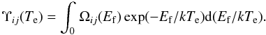${\mathrm{{\rm Y}}}_{\mathit{ij}}\mathrm{\left(}{\mathit{T}}_{\mathrm{e}}\mathrm{\right)}\mathrm{=}{\mathrm{\int }}_{\mathrm{0}}^{}{\mathrm{\Omega }}_{\mathit{ij}}\mathrm{\left(}{\mathit{E}}_{\mathrm{f}}\mathrm{\right)}\exp \mathrm{(}\mathrm{-}{\mathit{E}}_{\mathrm{f}}\mathit{/}\mathit{k}{\mathit{T}}_{\mathrm{e}}\mathrm{)}\mathrm{d}\mathrm{(}{\mathit{E}}_{\mathrm{f}}\mathit{/}\mathit{k}{\mathit{T}}_{\mathrm{e}}\mathrm{)}\mathit{.}$(2)

4. Results and discussion

In this section, in Figs. 1 − 3, we show a selection of collision strengths and their corresponding effective collision strengths. The transitions shown are typical of the kind of agreement and the types of differences we see between a distorted wave calculation and an R-matrix calculation. We also give a table which compares the effective collision strengths from the current calculation with those from Pradhan (1988) at three different temperatures (log₁₀ T_e = 5.0, 6.0, 7.0) for the transitions within the first ten fine structure levels – see Table 4.

The effective collision strengths presented are based on the collision strength data computed up to 2000 Ryd, since this is our most complete set. We find that for some transitions, the effective collision strengths are somewhat sensitive to the extending/truncating of the higher energy values of the collision strengths, particularly those where the high energy values dominate the collision strength. However, the differing energy determinations yield almost identical effective collision strength data up to the temperature log ₁₀T_e(K) = 7.0, and it is only above this temperature that differences are detected, if at all. All our sets include high energy limits which for each transition remain constant from run to run, however the “shape” of the high energy tail may alter slightly when comparing an extrapolated collision strength with one where high energy values are explicitly determined. Thus we are confident with our results up to log ₁₀T_e(K) = 7.0, but at higher temperatures we are less confident as we see some values change when the energy range is extended.

Table 5¹ gives our complete set of effective collision strengths for all 666 transitions produced in this work and contains the following information: Col. 1 lists the transition index noted as i − j (initial–final level) where the levels are given in the accompanying table and correspond to those in Table 2. The remaining columns list the effective collision strengths for each transition at logarithmic electron temperatures log ₁₀ T_e(K) = 4.5–8.0 in steps of 0.5 dex².

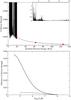Fig. 1 Transition 1−2: 3s${}^{\mathrm{2}}\hspace{0.17em}^{\mathrm{1}}$S0 − 3s3p   3P$\begin{array}{}\mathrm{◦}\\ \mathrm{0}\end{array}$Upper graph collision strengths: – current R-matrix results; • distorted wave results of Christensen et al. (1986). Lower graph effective collision strengths: – current R-matrix results; – distorted wave results of Pradhan (1988).

Transition 1−2: 3s${}^{\mathrm{2}}\hspace{0.17em}^{\mathrm{1}}$S₀ − 3s3p   ³P$\begin{array}{}\mathrm{◦}\\ \mathrm{0}\end{array}$ The data for transition 1 − 2 is shown in Fig. 1. Here the collision strength, for the current R-matrix calculation has an immense amount of resonance structures from threshold up to the energy of the highest target state included (3s4s ¹S₁ at 20.1689 Rydbergs). The inset on this graph shows how the resonances dominate the collision strength and that they are huge in magnitude compared to the background level of the collision strength in the high energy region. Comparing this high energy background level between the two calculations at the energies of 19.96, 62.983 and 125.966 Rydbergs where the distorted wave calculation provides evaluations, we see good agreement with the current R-matrix results.

The impact of the resonance stuctures can be clearly seen in the effective collision strength plot, where under the integration noted by (2) the height of the low-lying resonances enhances the effective collision strength at low temperatures. At high temperature, the since the background level of the collision strengths in the two calculations are in good agreement, we see that the effective collision strength also exhibits good agreement.

Transition 1 − 3: 3s${}^{\mathrm{2}}\hspace{0.17em}^{\mathrm{1}}$S₀ − 3s3p   ³P$\begin{array}{}\mathrm{◦}\\ \mathrm{1}\end{array}$ The data for this transition is shown in Fig. 2. In the collision strength plot, again we see that the resonances dominate in the low energy region. For the background level, on comparison with the values from the distorted wave calculation, we see that the R-matrix results are a factor of 2 − 3 higher.

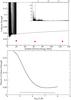Fig. 2 Transition 1−3: 3s${}^{\mathrm{2}}\hspace{0.17em}^{\mathrm{1}}$S0 − 3s3p   3P$\begin{array}{}\mathrm{◦}\\ \mathrm{1}\end{array}$Upper graph collision strengths: – current R-matrix results; • distorted wave results of Christensen et al. (1986). Lower graph effective collision strengths: – current R-matrix results; – distorted wave results of Pradhan (1988).

This leads to the effective collision strengths in the two calculations being quite different in shape and magnitude. As in the previous transition, the large resonance structures in the collision strength cause the effective collision strengths of the R-matrix calculation to be enhanced at low temperatures, and the absence of this detail in the distorted wave calculation means that the effective collision strength remains low in this region. At higher temperatures for this transition the two calculations do not converge as seen in the previous transition. This is due to the divergence of the collision strengths, and a similar factor of 2 − 3 is observed as a difference in the effective collision strengths. There is a slight upturn in the effective collision strength at high temperatures which occurs when we allow the collision strength whose tail section steadily increases to continue to the energy of 2000 Ryd before applying the extrapolation to the high energy limit.

Transition 1 − 5: 3s${}^{\mathrm{2}}\hspace{0.17em}^{\mathrm{1}}$S₀ − 3s3p   ¹P$\begin{array}{}\mathrm{◦}\\ \mathrm{1}\end{array}$ The data for this transition is given in Fig. 3. The collision strengths are in reasonable agreement, with the three distorted wave values lying slightly above those of the R-matrix. It is noted for this transition, on examining the main collision strength plot and the inset, that the resonances do not dominate the collision strength to the same extent as the two previous transitions; in fact the high energy tail section attains a magnitude that is greater than much of the resonant structure. This increasing tail leads to an increase in the effective collision strength, which is observed in both calculations. Once again the continuation of our collision strength to 2000 Ryd with the increasing tail section leads to enhancement in the high temperature extremity of the effective collision strength.

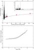Fig. 3 Transition 1 − 5: 3s${}^{\mathrm{2}}\hspace{0.17em}^{\mathrm{1}}$S0 − 3s3p   1P$\begin{array}{}\mathrm{◦}\\ \mathrm{1}\end{array}$. Upper graph collision strengths: – current R-matrix results; • distorted wave results of Christensen et al. (1986). Lower graph effective collision strengths: – current R-matrix results; – distorted wave results of Pradhan (1988).

The general trend from the plots displayed in Figs. 1 − 3 and from the “Current/Pradhan” ratios displayed in Table 4 is that the effective collision strengths from the R-matrix calculation we have performed are significantly enhanced by the resonances, particularly at lower temperatures, and are larger than the Distorted Wave values by up to a factor of 37 as noted for the 3s3p³P$\begin{array}{}\mathrm{◦}\\ \mathrm{1}\end{array}$ − 3s3p¹P$\begin{array}{}\mathrm{◦}\\ \mathrm{1}\end{array}$ transition.

5. Conclusions

Collision strengths and effective collision strengths for 666 transitions have been generated. A few selected transitions are discussed here. Differences exist between the current values and those from distorted wave evaluations, in general we find resonance contributions in our collision strengths greatly enhance the effective collision strengths.

As noted in the previous section, for some transitions, the reliability of the high temperature results may be questionable as there is some sensitivity to where the collision strength is truncated and the extrapolation to the high-energy limit begins. Certainly, the accuracy of the collision strengths would improve by obtaining a better shape for the high energy tail by considering a larger calculation and including additional target levels. The current data is consistent over all energy regions considered up to log ₁₀T_e(K) = 7.0.

The effective collision strengths are available at the CDS or alternatively the collision strength and effective collision strength data are available by contacting the author or via the website www.am.qub.ac.uk/apa.

Acknowledgments

This work has been supported by PPARC/STFC, under the auspices of a Rolling Grant.

References

All Tables

All Figures

	Fig. 1 Transition 1−2: 3s${}^{\mathrm{2}}\hspace{0.17em}^{\mathrm{1}}$S0 − 3s3p   3P$\begin{array}{}\mathrm{◦}\\ \mathrm{0}\end{array}$Upper graph collision strengths: – current R-matrix results; • distorted wave results of Christensen et al. (1986). Lower graph effective collision strengths: – current R-matrix results; – distorted wave results of Pradhan (1988).
In the text

	Fig. 2 Transition 1−3: 3s${}^{\mathrm{2}}\hspace{0.17em}^{\mathrm{1}}$S0 − 3s3p   3P$\begin{array}{}\mathrm{◦}\\ \mathrm{1}\end{array}$Upper graph collision strengths: – current R-matrix results; • distorted wave results of Christensen et al. (1986). Lower graph effective collision strengths: – current R-matrix results; – distorted wave results of Pradhan (1988).
In the text

	Fig. 3 Transition 1 − 5: 3s${}^{\mathrm{2}}\hspace{0.17em}^{\mathrm{1}}$S0 − 3s3p   1P$\begin{array}{}\mathrm{◦}\\ \mathrm{1}\end{array}$. Upper graph collision strengths: – current R-matrix results; • distorted wave results of Christensen et al. (1986). Lower graph effective collision strengths: – current R-matrix results; – distorted wave results of Pradhan (1988).
In the text

References

- Aggarwal, K. M., Tayal, V., Gupta, G. P., & Keenan, F. P. 2007, Atomic Data and Nuclear Data Tables, 93, 615 [Google Scholar]
- Burgess, A., Hummer, D. G., & Tully, J. A. 1970, Phil. Trans. R. Soc. Lond. A, 266, 225 [Google Scholar]
- Christensen, R. B., Norcross, D. W., & Pradhan, A. K. 1986, Phys. Rev. A, 34, 4704 [NASA ADS] [CrossRef] [Google Scholar]
- Dyall, K. G., Grant, I. P., Johnson, C. T., Parpia, F. A., & Plummer, E. P. 1989, Comput. Phys. Commun., 55, 425 [NASA ADS] [CrossRef] [Google Scholar]
- Grant, I. P., McKenzie, B. J., Norrington, P. H., Mayers, D. F., & Pyper, N. C. 1980, Comput. Phys. Commun., 21, 207 [NASA ADS] [CrossRef] [Google Scholar]
- Ralchenko, Yu., Kramida, A. E., Reader, J., & NIST ASD Team 2008, NIST Atomic Spectra Database. Available: http://physics.nist.gov/asd3. National Institute of Standards and Technology, Gaithersburg, MD. [Google Scholar]
- Pradhan, A. K. 1988, Atomic Data and Nuclear Data Tables, 40, 335 [Google Scholar]
- Saraph, H. E. 1972, Comput. Phys. Commun., 3, 256 [Google Scholar]
- Saraph, H. E. 1978, Comput. Phys. Commun., 15, 247 [Google Scholar]
- Ait-Tahar, S., Grant, I. P., & Norrington, P. H. 1997, Phys. Rev. Lett., 79, 2955 [NASA ADS] [CrossRef] [Google Scholar]
- Young, P. R., del Zanna, G., Mason, H. E., et al. 2007, PASJ, 59, S857 [NASA ADS] [CrossRef] [Google Scholar]
All Tables
Transitions energies/wavelengths (λ in Å), radiative transition rates (A in s-1), absorption oscillator strengths (f, dimensionless) and line strengths (S in a.u.) for E1 transitions from the 3s2 and 3s3p levels, from the current work along with values from Christensen.
Effective collision strengths for transitions between the 3s2, 3s3p and 3p2 fine structure levels at log 10Te(K) = 5.0, 6.0 and 7.0 from the calculation of Pradhan compared to those of the current work.