| Issue |
A&A
Volume 537, January 2012
|
|
|---|---|---|
| Article Number | A99 | |
| Number of page(s) | 13 | |
| Section | Catalogs and data | |
| DOI | https://doi.org/10.1051/0004-6361/201117954 | |
| Published online | 16 January 2012 | |
The second release of the Large Quasar Astrometric Catalog (LQAC-2)⋆
1 Observatoire de Paris, SYRTE/UMR-8630 CNRS, 75014 Paris, France
e-mail: Jean.Souchay@obspm.fr
2 Observatorio Nacional/MCT, Rio de Janeiro / Observatorio do Valongo; UFRJ, Rio de Janeiro, Brazil
3 Osservatorio astronomico di Torino INAF/OATo, Italy
Received: 26 August 2011
Accepted: 13 October 2011
Context. Since the first release of the LQAC (Large Quasar Astrometric Catalogue) a large number of quasars have been discovered through very dense observational surveys. As these objects constitute the cornerstones of modern astrometry by indicating quasi inertial directions, their spatial density and their astrometric quality must be studied in detail.
Aims. Following the same procedure as in this first release of the LQAC, our aim is to compile all the quasars recorded until the present date, with the best determination of their equatorial coordinates in the ICRS, i.e. with respect to the newly established ICRF2 and with the maximum of information concerning their physical properties (redshift, photometry, absolute magnitudes).
Methods. First of all we made a substantial review of the definitions and properties of quasars and AGN (active galactic nuclei), because the differenciation of these objects is unclear in the literature, even for specialists. Then we carried out the cross-identification between the nine catalogs of quasars chosen for their accuracy and their huge number of objects, including all the available data related to magnitudes, radiofluxes, and redshifts. Moreover, we computed the absolute magnitude of our extragalactic objects by taking the recent studies concerning the galactic absorption into account. In addition, substantial improvements were made with respect to the first release of the LQAC. First, an LQAC name is given for each object based on its equatorial coordinates with respect to the ICRS, following a procedure that creates no ambiguity in the identification. Second the equatorial coordinates of the objects were recomputed more accurately according to the algorithms used for the elaboration of the Large Quasar Reference Frame (LQRF). Third we introduce a morphological classification for the objects that in particular clearly defines if the object is point-like or extended.
Results. Our final catalog, called LQAC-2, contains 187 504 quasars. This is roughly 65% more than the 113 666 quasars recorded in the first version of the LQAC and a little more than the number of quasars recorded in the updated version of the Véron-Cetty & Véron (2010, A&A, 518, A10) catalog, which was the densest compilation of quasars up to now. In addition to the quantitative and qualitative improvements brought by our compilation, we discuss the homogeneity of the data and carry out statistical analysis of the spatial density and the distance to the closest neighbor.
Conclusions. The LQAC-2 will be useful for the astronomical community since it gives the most complete information available about the whole set of already recorded quasars, insisting on the precision and accuracy of their coordinates with respect to the ICRF-2.
Key words: cosmological parameters / astrometry / quasars: general / catalogs
The catalog is only available in electronic form at the CDS via anonymous ftp to cdsarc.u-strasbg.fr (130.79.128.5) or via http://cdsarc.u-strasbg.fr/viz-bin/qcat?J/A+A/537/A99
© ESO, 2012
1. Introduction
Quasars a priori materialize quasi-inertial directions in space, and for this reason they represent ideal objects for modern astrometry. As they are supposed to undergo no detectable proper motion on contrast to stars, they constitute the basis of a primary reference frame, as is the case of the ICRF2 (Ma et al. 2009; Boboltz et al. 2010). Since the identification of the first quasar 3C 273 by Maarten Schmidt in 1962 as an extragalactic radiosource with high redshift and the construction of the first quasars catalog by De Veny et al. (1971) containing 202 objects, the number of known quasars has steadily increased, in particular in the past decade, thanks to huge surveys like the 2dF QSO’s survey (Croom et al. 2004) and for a large part to the Sloan Digital Sky Survey (Fan et al. 1999; Adelman-Mc.Carthy et al. 2006). Nowadays the number of recorded quasars that can be compiled reach more than 180 000 objects. Considering this dramatic increase, once in a while one needs to gather all the quasars into a single catalog that is as homogeneous as possible. This has been done for a long time through several releases by Véron-Cetty and Véron from 1984 to 2010. In parallel, Souchay et al. (2009) have constructed what they call the LQAC (Large Quasar Astrometric Catalogue), which can be considered as an alternative catalog to the one from Véron-Cetty & Véron (2006), which was the densest catalog of quasars available at the time.
Some advantages can be found in the LQAC. First, it is oriented towards astrometric reliability and performance as its name shows it. For the sake of homogeneity, it systematically privilegies large surveys over small catalogs. Second it is based on a compilation strategy related to the astrometric level of the constituent catalogs; in other words, when an object is available in two or more catalogs, only the positions (in terms of celestial coordinates) provided by the most accurate catalog are retained. Third the LQAC contains exhaustive information on the photometry of the objects, thanks to crossidentifications between the constituent catalogs as well as between large surveys such as the 2MASS catalog (Cutri et al. 2003), the USNO B1.0 catalog (Monet et al. 2003) or the GSC2.3 catalog (Lasker et al. 2008). Finally the LQAC determines the absolute magnitudes of quasars in both bands i and r, by using up-to-date models of galactic extinction and recent values of cosmological parameters.
Several reasons led us to construct a new version of the LQAC, called the LQAC-2. At first we considered a significant amount of new data from different origins, such as the ICRF2 (Ma et al. 2009; Boboltz et al. 2010) and the VCS (Petrov et al. 2008) at radio wavelengths, as well as the 8th release (DR8) of the Sloan Digital Sky Survey at optical wavelengths (Aihara et al. 2011). A second important reason is to include the equatorial coordinates of the quasars as determined from the LQRF (Large Quasar Reference Frame), which a priori gives a more accurate optical determination of celetial coordinates with respect to the ICRF (Andrei et al. 2009), compared with those given by original catalogs, for a high percentage of objects (except of course those observed with the VLBI). Finally another reason comes from a decision to densify the data compared to the first LQAC catalog. One of the improvements is to include an LQAC identification number based on the celestial coordinates of the objects. Another significant improvement is to determine three kinds of indexes, thereby allowing a morphological classification. These indexes are obtained by comparison to the average morphology of the surrounding stars, thus freed of image aberrations. They are obtained from B, R, I images and their first interpretation is to point out the signature of the host galaxy.
Before explaining the contents of the LQAC-2 in full details, in Sect. 2 we substantially review the basic considerations about quasars and their link with objects such as AGN (active galactic nuclei), BL LAC or Seyfert galaxies. Then in Sect. 3 we describe the construction and the contents of the 9 quasars catalogs used in our compilation, as well as three all-sky surveys. This enables us to add substantial photometric information on the recorded objects. Some of the catalogs have not changed since our first LQAC compilation, so that we do not dwell on them. Others are new releases or simply new catalogs which on the contrary deserve substantial description.
In Sect. 4 we explain how we compiled the LQAC-2 starting from a well-established cross-identification algorithm applied for the catalogs involved. We give some details about how we solved the delicate case of the Hewitt & Burbridge (1993) catalog (quoted as HB in the following) characterized by a lack of astrometric accuracy of an important part of the relevant quasars. Then we present our method of determining the absolute magnitudes of the objects.
In Sect. 5 we give the improvements brought by the LQAC-2 over the first LQAC. Some of them are simply quantitative such as the increase in the total number of quasars in our compilation and consequently of the number of cross-identifications between catalogs. Moreover we add new information for the recorded objects, such as the creation of an identification number, the introduction of coordinates given in the LQRF (Andrei et al. 2009), which are generally more accurate than those given in the original catalogs, and the determination, when it is available, of morphological indexes characterizing the the apparent image of the quasar (normalness, roundness, skewness)
Finally Sect. 6 provides a short statistical study of the spatial distribution of the LQAC-2 objects, as well as a specific analysis for the closest neighbor.
2. Definition of quasars
Since our objective is to gather all the recorded quasars, it is worth considering their definition and the possibility that other kinds of objects fit this definition. Without this preliminary step and clear selction criteria, our compilation procedure would become ambigous. This is made even more compulsory by the lack of unity and coherence in the definitions of “quasar” generally used in the literature.
2.1. A brief historical reminder
The first quasar was discovered in the late 1950’s, as a radio source with no corresponding visible object. A few years later, in 1960, a point-like counterpart was found for the quasar 3C 48. Nevertheless, its emission lines were so redshifted that they were not recognized. A giant step was made in 1962, when Marteen Schmidt analyzed the spectrum of 3C 273 and understood for the first time that the emission lines were redshifted spectral lines of hydrogen. Gradually the terminology of quasar was extended as well to objects with a compact appareance and high redshifts, which are only detected at optical wavelengths. Some similar objects with starlike resolution and radio emission had been found, so that and Hong-Yee Chiu adopted the term quasar in Physics Today in May 1964, to avoid the long and cumbersome full term quasi-stellar radio source.
At that point, the meaning of the term quasar was not relevant anymore since some of those “radio sources” were actually not radio loud. In parallel the new terminology of QSO appeared, standing for quasi stellar object, and included all the objects that could not be resolved, either because they were too far away or too small (or both). Later observations indeed pointed the existence of different types of quasi stellar objects that shared properties with quasars: radiogalaxies, Seyfert galaxies, and blazars, for instance.
2.2. The unified active galaxy nucleus model
To be able to choose observational criteria for defining a quasar, it is compulsory to understand the physical object that emits the measured signals. The physical explanation of a quasar is now relatively well established and relies on the AGN model. An AGN is believed to represent the compact region in the center of a massive galaxy, close to its central supermassive black hole (typically with a mass 106–109 M⊙), and powered by an accretion disk surrounding it. Constraints exerted on the accreted matter turn it into an ionized plasma, whose motion creates a transverse magnetic field. Some particles can be accelerated by this field and expelled from the disk. They form two transversal jets that end in huge lobs. In their motion, they emit the powerful radio signal observed sometimes. The bulk optical emission could be explained by the gravitational energy released because of the black hole. Such an object has a specified axis, transverse to the accretion disk. Depending on the observational angle towards the axis and the intensity of the emissions (probably linked to the age of the object), this model would give one of the aforementioned classes of QSO’s to see.
Thus in the framework of the unified theory, classification of AGN’s is largely a matter of a line-of-sight perspective. Naturally, a less schematic classification must consider such particularities as the object interaction and merger history, the dust content, the star formation waves, the rate and gyro direction of the central massive black hole, and the enrichment of the accretion disk shells or regions. Nonetheless, the entrusted relationship between the mass of the central black hole, its luminosity, and the mass and luminosity of the host galaxy must generally hold. Therefore since quasars are essentially quasi stellar objects from optical ground observations, an apparent paradox arises: generally the more massive and luminous a host galaxy is, the more luminous the quasar tends to be, thus making the host galaxy invisible in contrast, even if this effect is to some extent modulated by its relationship to the viewing direction. Hubble images and active optics now enable study of the host galaxy, which increases the knowledge about the quasar itself, too. The presence of the host galaxy can also be inferred from color studies (Sakata et al. 2010) and from departures in the compound PSF (point spread function) of the quasar as well as the host galaxy to the purely pointlike stellar PSF’s (Falomo et al. 2001). This methodology can be used to morphologically classify the quasars observed from outside the atmosphere, as will be the case for the Gaia mission, hence deriving an astrometrically more precise centroid than if a stellar PSF had been applied for the centroid determination.
2.3. Definition used in this paper
In their recent catalog updates, Véron-Cetty & Véron (2006, 2010) define a quasar as a starlike object or as an object with a starlike nucleus with broad emission lines and with an absolute magnitude below a given threshold M0. This is a purely arbitrary definition that also depends on the changes in the value of fundamental cosmological parameters considered for determining the absolute magnitude. For instance, we can see that in the two updates mentioned above the magnitude threshold M0 was shifted from M0 = −23.00 to M0 = −22.25 when considering the change of the Hubble constant from H0 = 50 km s-1 Mpc-1 to H0 = 71 km s-1 Mpc-1. The disadvantage of adopting this kind of conventional definition is both that it does not seem to correspond to any discontinuity in the physical nature of the object and that it is directly dependent on cosmological parameters and of their revision.
As a result, we decided to use an effective definition of “quasars” that would not rely on those arbitrary cosmological parameters. We therefore call “quasar” any object that can be seen as a classical quasar from a given point of view and with a specific set of image parameters. We are well aware this defintion may include some AGN usually sorted as Seyfert galaxies or radio galaxies, and yet it seems consistent with our aim of gathering data on a specific physical object.
In the paper devoted to their last catalog update, Véron-Cetty & Véron (2010) point out that some objects present in the LQAC (Souchay et al. 2009) were not strictly quasars for they have no optical identification or measured redshift. They refer to 2921 objects observed by the radio VLBI technique present in the ICRF2, VLBA, VLA, and JVAS catalogs (with respective flags A, B, C and D). These objects can indeed be considered as quasars because their radio emission and core-dominated VLBI radio map structure at the mas (milliarcseond) level is like other radio-loud QSO’s that possess an optical counterpart.
Moreover, when considering the unified AGN model (see Sect. 2.2) we decided to include AGNs recorded in several catalogs, and in particular the large number included in Véron-Cetty & Véron (2010). They are either Seyfert 1s or Seyfert 2s galaxies, where the first ones are characterized by broad Balmer and other permitted lines, the second ones by Balmer and forbidden lines of the same width. A more subtle classification of Seyferts galaxies can be found in that paper. The authors indicate clearly that some objects would move from the QSO classification to the AGN one, and vice versa, if other values of the cosmological parameters q0, H0 and of spectral index were used or if a more accurate B apparent magnitude was available.
3. The catalogs participating in the LQAC-2 compilation
3.1. The ICRF2
The second realization of the International Celestial Reference Frame, called the ICRF2 (Ma et al. 2009; Boboltz et al. 2010) was generated by using 30 years of VLBI (Very Long Baseline Interferometry) observations. It contains positions of 3414 compact radio sources, which correspond to more than five times the number of objects in the first version of the ICRF, namely ICRF1 (Ma et al. 1998). The improvement also concerns the astrometric accuracy. The ICRF2 is found to have a noise floor for positions of radio sources of only ≈40 μas (microarcseconds), which is five or six times better than the ICRF1. The axis stability is around 10 μas, which is nearly twice as stable as the ICRF1. The alignment of the ICRF2 to the ICRF1, neede to respect the basic principles of the ICRS (International Celestial Reference System) was made using 138 stable sources common both to the ICRF1-Ext.2 (Fey et al. 2004) and the ICRF2. A set of 295 new defining sources was selected on the basis of both positional stability and lack of intrinsic source structure. These sources have a more uniform sky distribution and better stability as in the case of the ICRF1.
3.2. The VLBI global solution rfc2010d
The VLBI astrometric global solution rfc2010d used all the available VLBI observations at 8.6 GHz and 2.2 GHz, as well as 5 and 22 GHz from April 1984 to June 2010. These observations were done during 5017 24-h sessions, including 64 VLBA observing sessions dedicated to the absolute astrometry surveys, such as the VLBA Calibrator Survey (VCS), the VLBA Galactic Plan Survey, the Australian LBA Calibrator Survey, the IFGL AGN4s on parsec scales, VLBI2MASS radioastronomy project, and the EVN Galactic Plan Survey. The total number of delays in this rfc2010d update reaches 8027588 estimates.
The largest program, the VCS (Petrov 2008), has played a considerable role in the astrometric performance. Indeed, the possibility of reaching microarcsecond VLBA astrometry depends on the presence of suitable calibrators with coordinates known at sub-mas level within several degrees from targets. In the past 15 years, significant efforts have been made to build a catalog of around 4000 calibrators. Recently optimization of source selection and observing schedules significantly increased the number of detected sources and reduced systematic errors of position estimates.
3.3. The Very Large Array and the Jodrell Bank-VLA Astrometric Survey
We used exactly the same versions of the catalogs from the Very Large Array (VLA) and the Jodrell Bank VLA Astrometric Survey (JVAS) as in the first release of the LQAC (Souchay et al. 2009). They contain 1858 and 2118 extragalactic radio sources respectively. General information concerning these two catalogs are summarized in this last paper. Details for the VLA can be found in Claussen (2006) and from the corresponding manual (http://www/aoc.edu/~gtaylor/csource.html).
3.4. The Sloan Digital Sky Survey (SDSS)
The Sloan Digital Sky Survey (SDSS) is one of the most ambitious and influential surveys in the history of astronomy. In Operation for more than eight years it obtained deep, multi-color images covering more than a quarter of the sky with three dimensional maps of the universe containing a little less than 1 million galaxies and more than 120 000 quasars. The construction of the survey started from a dedicated 2.5 m telescope located at Apache Point, New Mexico, USA. Images are obtained in five broad optical bands (designated u, g, r, i, z) covering the wavelength range of the CCD response from atmospheric ultraviolet cut-off to the near infrared (Fukugita et al. 1996). The present SDSS-III, a program of four new surveys, began its observational sessions in July 2008, and will continue through 2014. More information on the SDSS-III can be found on the web site http://www.sdss3.org/. The SDSS quasars catalog used here comes from the first data release of the SDS-III and the eigth data release (DR8) counting from the beginning of the SDSS (Aihara et al. 2011). This five band imaging release includes a new 5200 deg2 area in the Southern Galactic cap, bringing the total area of the SDSS imaging to 14 555 deg2, roughly a third of the celestial sphere. The various quasars sub-catalogs coming from successive releases (from DR1 to DR8) of the SDSS show some incoherence for a significant amount of objects disappear from one given release to the next one, for various reasons (Schneider et al. 2010): for instance suspected pairs arising from cross matchning the DR5 and the DR7 and showing offsets larger than 1 arcsec were exluded for safety, and changes in the photometric measurements dropped the luminosity below the absolute magnitude criterion for quasar selection. Therefore instead of packing all the quasars present in some releases and not in other ones, as was done in the Véron-Cetty & Véron (2010) compilation procedure, we only considered the last release (DR8) as the reference for our compilation.
3.5. The 2dF Quasar Redshift Survey (2QZ)
This survey, still named 2QZ, is based on a preselection of quasars starting from u, bj, r broadband colors photographic plates (Croom et al. 2004). Their magnitude is ranged in the interval 16 < bJ < 20.9. The survey concerns two 75° × 5° declination strips passing across the south and the north Galactic caps. A second step consists in a spectroscopic follow-up with recognition starting from quasars spectra templates.
3.6. The 2dF-SDSS LRG and QSO (2SLAQ) Survey
The 2SLAQ Survey, which stands for the 2dF-Sloan Digital Sky Survey luminous red galaxy (LRG) and QSO Survey (2dF-SDSS LRG and QSO) (da Angela et al. 2008), is an extension of the previous 2QZ survey at fainter magnitudes. For the main aspects of this survey, we can refer to the explanations in Richards et al. (2005), who give the results of the first semesters of data collection with the corresponding luminosity function for a sample of roughly 5600 QSOs. Nowadays, the survey has been extended to a total of around 9000 QSO’s, with z < 3. The strategy of the survey consisted in combining photometric and spectroscopic data from the same objects, from the Sloan telescope and from the 2dF one respectively. The sky regions covered by the 2dF instrument consist of two 2° wide equatorial strips containing QSO candidates, observed by the SDSS survey. Spectroscopic fibers were allocated simultaneously to the LRGs (luminous red galaxies) linked to the red spectrograph and to the QSOs linked to the blue spectrograph. The two strips were located in the north Galactic cap (NGC) and the south galactic cap (SGC). In the NGC, 6680 objects (57.9%) were classified as QSOs whereas 2977 ones (18.0%) were identified as NELGs (narrow emission line galaxies) and 1829 ones (15.9%) as stars. In the SGC the numbers are respcetively 2378 QSO’s (49.7%), 905 NELG’s (18.9%), and 835 stars (17.4%).
3.7. The FIRST catalog
The FIRST catalog is the result of three successive releases that consist in matching a radio catalog, the NRAO VLA survey (Becker et al. 1995; Becker et al. 2001) with an optical catalog provided by the automated plate machine digitization of the Palomar Sky Survey Plates. The optical selection was refined by the intermediary of several spectroscopic campaigns.
3.8. The Hewitt and Burbridge catalog
The Hewitt & Burbridge (1993) catalog, here denoted as the HB catalog, was completed in 1992, and contains a majority of the quasars known at this epoch with corresponding redshifts, together with about 90 BLAC objects. Much information is contained in this catalog, such as celestial coordinates, colors, magnitudes, emission-line redshifts, absorption, variability, polarization as well as X-ray, radio, and infrared data, when available. As noticed and shown by Souchay et al. (2009), this catalog is far from being satisfactory from an astrometric point of view, because the celestial coordinates for a good amount of objects are not accurate. Souchay et al. (2009) showed that a search radius of 30 arcsec was sometimes necessary to cross-identify the objects of HB with other catalogs, whereas a search radius of one to two arcseconds was enough for crossidentification between the other catalogs. Therefore the possibility of a mismatch between two objects where one of them belongs to the HB catalog is very high. It was partially solved by comparing redshifts in Souchay et al. (2009). Here to remedy this lack of accuracy of the positioning of the objects in the HB catalog, we rely on our own specific algorithms of cross identification with other catalogs described in full details in Sect. 4.3.
3.9. Complementary information from the USNO B1.0, the GSC2.3, and the 2MASS catalogs
The three all-sky surveys USNOB1.0 (Monet et al. 2003), GSC2.3 (Lasker et al. 2003) and 2MASS (Cutri et al. 2003) will not bring any additional quasar for our compilation, but thanks to cross-identifications, they add significant new photometric information, filling a substantial amount of gaps in the data. The USNO-B1.0 catalog (Monet et al. 2003), as well as the GSC2.3 catalog (Lasker et al. 2008) come both from photographic plates and contain around 1 million objects each, add B, R, I magnitudes to our compilation, whereas the 2MASS catalog (Cutri et al. 2003) results from an all-sky infrared survey working at J, H, and Ks bands, to a 3 − σ sensitivity of 17.1, 16.4, and 15.3 mag, respectively.
3.10. The Véron-Cetty and Véron catalog
Recently, Véron-Cetty & Véron (2010) have published the 13th edition of their catalog of quasars, quoted in the following as VV2010 and itself consisting in a compilation of all the quasars discovered up to now, including those coming from vey small catalogs, some of them containing only a few objects. As our compilation procedure in this paper is essentially based on the using of only nine catalogs, characterized either by their very good accuracy (as the ICRF2) or by their large dataset (as the SDSS), we cannot avoid missing a significant number of objects that are not included in any of the nine catalogs above. Therefore we rely on the VV2010 catalog to add these missing quasars. Finally 22 440 objects were picked up from the VV2010 catalog to complete our LQAC-2 catalog, which represents 11.96% of the total number of quasars included. Among these 22 440 objects, 7869 are classified as QSO’s and 14 571 as AGN’s.
On the other hand, we did not take all the VV2010 quasars coming from the SDSS into account, that is to say, 88274 objects which represent 52.25% of the whole VV2010 catalog. The rationale of this choice is that the SDSS quasars in VV2010 come from various releases of the SDSS and that for the reasons already explained in Sect. 3.4, a significant number of them were not present in the last DR8 release, maybe because their existence as a quasar is doubtful. This choice does not affect the completness of the LQAC-2, for the SDSS (DR8) catalog is included in our compilation (flag “E”).
Characteristics of the catalogs participating to our compilation of quasars both for the LQAC-2 and the LQAC.
4. Construction of the LQAC-2 catalog
4.1. Nomenclature
As in the first version of the LQAC, we define a code characterized by a letter for each of the catalogs belonging to the compilation. The A-to-M codes for these individual catalogs are provided in Table 1, together with their nature (infrared, radio, and/or optical), the number of quasars and the respective number in the first version of the LQAC. These codes do not systematically correspond to the same individual catalog of the first version. For instance, flag A is corresponds to the ICRF2, whereas in the first version, it corresponded to the ICRF-Ext.2.
4.2. The cross-identification algorithm
Our method of carrying out the cross-identification between quasars belonging to two distinct catalogs is significantly different from and more sophisticated than the one used in the first version of the LQAC. Instead of fixing an arbitrary threshold (typically 1′′) of the angular distance beyond which two crossidentified objects are considered as distinct (instead of representing a single object), this threshold value is determined from a previous round of cross identifications, with a relatively high value of the threshold. The value of the rms σ of the angular distances is calculated. Then the rejection threshold is fixed to 5σ.
4.3. Solving the problem of the Hewitt and Burbridge catalog
The HB catalog (Hewitt & Burbridge 1993) contains 7245 quasars that we would like to include in the LQAC. Unfortunately a good part of them contain a very large positional uncertainty, very often exceeding 1′′ and sometimes reaching as much as 30′′. To assign accurate celestial coordinates to these quasars, an appropriate algorithmic treatment is necessary, based on two statistic criteria. We consider a given quasar of the HB catalog. First a cross identification with a large search radius Rmax, i.e. 60′′, is done between this quasar and the GSC2.3 catalog (which a priori contains stars as well as galaxies and quasars). If NT stands for the total number of objects of the GSC2.3 crossidentified in this 60′′ radius, and Rmin stands for the minimum distance for which a counterpart of the HB quasar has been found in the GSC2.3, then the probability of finding this counterpart is given by  (1)The slower the probability, the higher is the chance that the crossidentification between the HB quasar and the closest counterpart corresponds to a single object. Therefore as a first step we restrict our possible identification to couterparts for which P1 ≤ 1. In the case for where two or more quasar candidates have been identified, our algorithm leads to a second step: if we call
  the second closests object, we write
  (2)We want the distance that separates the HB quasar from the second closest object to be at least twice the distance Rmin to the closest neighbor, which is written: P2 ≤ 2. In the opposite case we consider that no counterpart has been found with enough certainty, so we reject any crossidentification with the GSC2.3. As a consequence, the HB quasar is not kept in the LQAC.
According to this second setp, 6721 quasars of the HB catalog were crossidentified with the GSC2.3 and could be recalibrated.astrometrically. This corresponds to 93% of the original sample containing 7245 quasars.
Number of cross-identified objects between the catalogs belonging to the LQAC.
4.4. Determination of luminosity distances and absolute magnitudes
We follow the same rules as in the first version of the LQAC to determine the absolute magnitude of a given quasar, from the following law:  (3)where M and m are respectively the absolute and apparent magnitudes of the quasars at a given bandwidth, DL is the luminosity distance, A represents the galactic extinction and K, traditionally called the K-correction is the effect of the redshift on the location of the spectrum corresponding to the filter through which M is determined.
As in Souchay et al. (2009), we computed the absolute magnitude in the blue band and in the infrared band, using the Hogg et al. (2000) formula for computing DL and the reddening value E(B − V) in magnitude based on the map of Schlegel et al. (1998) for computing the galactic extinction A. Moreover, the table provided by Véron-Cetty & Véron (priv. comm.) and one in Richards et al. (2006) are used for computing the K-corrections.
Nevertheless, in contrast to what we did in Souchay et al. (2009), and for reasons of photometric consistency, we only computed the blue absolute magnitudes of quasars for which a blue apparent magnitude is available in GSC2.3 and the infrared absolute magnitudes of quasars for which an infrared apparent magnitude is available in the SDSS (or possibly in the GSC2.3). We checked that for quasars in common with the first version of the LQAC, the comparison of the computed absolute magnitudes shows good agreement.
According to Hogg et al. (2000) in the case of an homogeneous and isotropic cosmological model with a Friemann-Lemaître-Robertson-Walker metrics with a null space curvature, the expression of the luminosity distance DL of a quasar with redshift z is given by:  (4)where c is the speed of light, H0 the Hubble expansion factor, and q0 a deceleration parameter. The dependence of the luminosity distance DL on the values of q0 and H0 was discussed by (Souchay et al. 2009). As in this last paper we adopt q0 = −0.58 and H0 = 72 km s-1 Mpc-1, consistent with recent cosmological constraints (Komatsu et al. 2011).
Photometry and redshift information from each optical catalog of the LQAC compilation.
Infrared photometry and radio flux informations available according to corresponding catalogs of the LQAC compilation.
5. Additions and improvements with respect to the first version of the LQAC
Our new catalog, LQAC-2, contains a total sample of 187 504 quasars in comparison to the 113 666 quasars compiled in the first version. In addition to this quantitative improvement (an increase of roughly 65% of the number of objects) new important items were added to the original information. First a reference number is given for each object, starting from its equatorial coordinates. Second an optimized determination of these coordinates starting from the LQRF (Andrei et al. 2009) is added in complement of the coordinates coming directly from the original catalog. These new coordinates, which were established with respect to the ICRF2, are generally more accurate than their original value. At last a morphological classification starting from three different indexes is done for a high proportion of the quasars of the LQAC-2. In the following we describe all the improvements mentioned above in details.
5.1. Crossidentifications between catalog
In Table 2, we show the number of crossidentifications for each pair of catalogs participating to the compilation. N = 13 being the number of the catalogs taken into account, we get (N − 1)N = 68 entries and N(N + 1) = 91 entries according to the case for which we consider the self crossidentifications or not. The two catalogs used for photometric completeness, the GSC2.3 and the B1.0, offer a large number of crossidentifications with the SDSS, 102 866 and 101 322 objects, respectively 81.3% and 80.0% of the total sample of 126 577 objects. In contrast, the number of radio-loud quasars (flags A to D) detected with the SDSS survey is quite poor with no more than 528 entries. Although many more SDSS quasars can be traced back in the VLA FIRST catalog (Schneider et al. 2010), those do not belong to the VLA list of calibrators and therefore are not crosscorrelated in the LQAC-2. In comparison, there are significantly more common radio-loud quasars (flags A to D) when the crosscorrelation is done with the GSC2.3 (2553 objects for the ICRF2, 3362 objects for the VLBA).
In Tables 3 and 4 we find the number of entries per catalog, for a given item concerning optical magnitudes and redshift (Table 3), infrared magnitude, and radio flux (Table 4). We note the possible redundancy of the information: the same item can be found within two or more different catalog for any given quasar. In that case, the priority by alphabetic order of the flags is retained. That is, for instance, the case of the 2140 quasars belonging both to the SDSS and the 2QZ catalogs, for which one value of the u magnitude or of the redshift is given in each. Therefore, obeying the rule, the information is taken fro both items from the SDSS (flag “E”) instead of the 2QZ (flag “F”).
Comparison of the number of entries for each data item between the VV2010 catalog, the compilation of the catalogs A-L and the final LQAC-2 catalog.
Table 5 shows the number of objects for which the information is availablefor each item involved in the compilation (optical or infrared magnitude, radio flux, redshift). We compared our results with the last version VV2010 of Véron & Cetty (2010) releases. Notice that 35 605 among the 168 941 objects of VV2010 are AGN’s, or roughly 21%. The larger number of quasars included in the LQAC-2 (187 504 instead of 165 065, that is to say a 13.5% increase) is essentially because the LQAC-2 has taken the eighth release of the SDSS (Aihara et al. 2011) into account, whereas the VV2010 catalog caught all the SDSS quasars up to the seventh release (DR7) (Abazajian et al. 2009). Redshifts are available for 98% of the total sample. Moreover, apparent magnitudes at optical wavelengths are significantly more complete in the LQAC-2 (1 021 554 entries in all, when including all the bandwidths) than in the VV2010 (321 133 entries) and infrared data in bands J and K concern 13.5% of the LQAC-2 objects, whereas it is not provided by VV2010.
5.2. A LQAC-2 number for each quasar
Since the average density of the LQAC-2 catalog is about 4.7 quasars per square degree, the probability of finding two really distinct objects from two different original catalogs at an angular distance less than 1′′ is quasi null (see Sect. 6). Therefore it could be practical and natural to designate each quasar by its equatorial coordinates calculated in degree and truncated to the arcsecond level. For instance, a quasar of our catalog with right ascension α = 243.457896° and declination δ = −25.352781° with respect to the ICRF could be designated as LQAC243.4579-25.3528. In fact, we can notice that this last kind of designation is particularly cumbersome and subject to mistakes because of the large number of digits. Thus we decided to arrange the quasars by interval of degree unit both in right ascension and declination and to give a sequential number for each bidimensional interval. Thus the quasar above is called LQAC243-25-1 if it is the first quasar to be identified in the range 243° < α < 244° and −26° < δ < −25°, or LQAC243-25-n if it is the nth quasar belonging to this same interval. This way of designation has several advantages. First it enables one to understand very quickly in which area of the sky the quasar is located. Second it does not involve a lot of digits, which is a source of error in identification. Finally it does not suffer from an update of the catalog: for instance if new quasars are identified in the bi-dimensional interval above in future LQAC releases, their sequential number will be incremented to n + 1, n + 2 etc. without affecting the previous designations.
5.3. Determination of coordinates from the LQRF
The LQRF (Large Quasar Reference Frame) was recently constructed (Andrei et al. 2009), taking care to avoid incorrect matches of its quasars, homogenizing astrometry from the different catalogs and reaching milliarcsecond global alignment with the ICRF. The quasars included in the LQRF were themselves taken from the LQAC (Souchay et al. 2009), whereas their positions were found, when available in the USNO B1.0 (Monet etal. 2003), GSC2.3 (Lasker et al. 2008), and SDSS Data Release 5 (Adelman-McCarthy et al. 2007). The positions were then placed onto the UCAC-2 based reference frames (Zacharias et al. 2004). Then the ICRF, VLBA, and VLA radio calibrator objects were used when optical counterpart existed, enabling direct matching between the radio and optical positions. This matching was used to derive the global orientation towards the ICRF and to determine spherical harmonics corrections and large scale warps.
Finally the celestial coordinates of the objects were determined homogenously in the ICRF frame with the intermediary of spherical harmonics. In its first version (Andrei et al. 2009) the LQRF contained 100 165 quasars, relatively well distributed across the celestial sphere, from − 83.5° to + 88° in declination. The average distance between adjacent elements is 10′. The global alignment with the ICRF is 15 milliarcseconds (mas) and the individual position accuracies are represented by a Poisson distribution peaking at 139 mas in right ascension and 130 mas in declination. One of the substantial improvements brought by the LQRF consists in significant corrections in the equatorial coordinates with respect to the determinations from the original optical catalogs, and and the determinination of their systematic departures from the ICRF. The procedure used to compute the LQRF was kept to determine the coordinates of the quasars present in the LQAC-2 and not in the LQAC, thus leading to a second version of the LQRF, called LQRF-2, which of course only contains quasars with optical counterparts. The only variation in the procedure was the adoption of the UCAC-3 and PPMXL reference catalogs (other than maintaining the 2MASS), and embeding the spherical harmonics determination into the final zonal warp removal.
5.4. The morphological characterization of the LQAC-2 sources
One of the important improvement of the LQAC-2 catalog with respect to the LQAC (Souchay et al. 2009) consists in including a morphological classification of the objects using the available B, R, and I DSS images. The DSS (Digital Sky Survey) is a collection of Schmidt plates covering the entire sky. The plates are dated from various epochs within the past 30 years. They have been scanned elecronically, providing multicolor, full sky coverage. The plates from the south hemisphere come mainly from the SERC (Science and Engineering Research Council) Southern Sky Survey and from the SERC J equatorial extension. Data from the northern hemisphere was obtained mainly from the 1950–1955 epoch Palomar Sky Survey.
The morphological classification derives from comparing the quasar point spread function (PSF) against the local, stellar PSF. A surrounding field of 5 × 5 arcmins around the quasar is obtained from the DSS B, R, and I plates. Since the corresponding neighborhood catalog has already been extracted for the steps explained in the previous section dealing with LQRF-2, it is easy to locate the quasar and nearby isolated stars, preferentially of similar magnitude. For the complete LQAC-2 sample we obtained images of 114 606 fields from the B plates, 191 030 from the R plates, and 183 421 from the I plates. The lack of information in most cases is due to incomplete sky coverage or to the lack of available uncompressed digitalization for the DSS2 blue plates, as well as to a residual number of faulty file transfers. In the retrieved plates some cases occur when a quasar is not present or too faint to provide a meaningful PSF (29 497 objects in the B plates, 37 790 objects in the R plates, and 29 799 objects in the I plates). At last, there were not enough adequate comparison stars in six B plates, in 134 R plates, and in 86 I plates. As expected, due to the more complete sky coverage and to the accessibility to fainter stars than for other filters, the most quasars correspond to the R plates.
The IRAF task DAOFIND is used both to find stars and targets, as well as to derive the PSF parameters. Additionally, the tasks from the IMMATCH IRAFťs package are used to match stars and targets to their catalog positions and magnitudes. Calibrating stars for the PSF are collected within one magnitude from the quasar magnitude, but when less than five stars are picked up, the magnitude limits are progressively enlarged in one magnitude step, except stars brighter than the tenth magnitude. Stars must be isolated from each other by an inner radius of ten pixels and within the frame by the same threshold. If rewer than five comparison stars are found, no morphological index is derived for that quasar on that plate. Three estimators of the PSF are used: SHARP (probing skewness), SROUND (probing roundness), and GROUND (probing normalness). The morphological indexes are given by (Andrei et al., in prep.):  (5)where IPC(Q) is the morphological index of quasar Q for the PSF parameter P in the color C, given in comparison to the mean value from the stars s, and normalized by the stellar standard deviation σ.
To test the power and efficiency of the above procedure applied to the DSS Schmidt plates, a comparative test was made using 1343 objects present on the DSS and the SDSS images (Andrei et al., in prep.). The large number of quasars enabled the SDSS space to be sampled regularly, corresponding to one fourth of the total celestial sphere, and the extreme examples with low and high redshifts, bright and faint magnitudes, and both tails of the color distribution. These many objects also allowed retaining only the quasars for which at least 20 comparison stars were found. The analysis showed that there is no degeneracy in the indexes with magnitude. All nine morphological indexes, namely three parameters in three colors, behaved alike on the DSS and SDSS.
We made a careful analysis of how the morphological indexes behave for stars and we found that only 1% of the stars were misidentified by the morphological indexes, while for the quasars the correlation between the morphological classification and the SDSS catalog classification was of 0.86 for the SDSS images and of 0.72 for the DSS images. Due to the better quality of the SDSS images and pixelization, the number of quasars reckoned as extremely non-pointlike is greater from the SDSS fields (144 objects) than from the DSS fields (86 objects), but 50% of the sample are common. Thus the trial described above supports using the DSS images to derive a morphological index, which describes the degree of agreement or disagreement of the quasars PSF to the mean local stellar PSF. Owing to the limited resolution, the morphological indexes are interpreted as presenting the signature of the host galaxy.
Table 7 brings the number of quasars for which the morphological indexes are presented. It also indicates the number of examined quasars that display, in a given plate color, a morphological index larger than 2, that is, 2 standard deviations off the local mean PSF characteristics. The relative distributions are shown in Figs. 1 to 3, respectively, for the SHARP, the SROUND, and the GROUND indexes. Both from the table and the figures, it is obvious that the number of non point-like quasars is small but by no means negligible. We found a relatively small number of non pointlike quasars in the B plates and progressively more in the R and I plates, which is expected from the redder emission from the host galaxy than from the inner quasar sources participating to the optical emission.
Number of morphological indexes and quantity of objects off 2σ from the local mean stellar PSF.
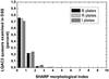 |
Fig. 1 Binned distribution of the morphological index SHARP. The color codes stand for the respective DSS plates. |
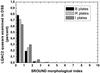 |
Fig. 2 Binned distribution of the morphological index SROUND. The color codes stand for the respective DSS plates. |
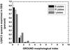 |
Fig. 3 Binned distribution of the morphological index GROUND. The color codes stand for the respective DSS plates. |
6. Statistical study
One of the most important characteristics we should require from a general compilation of quasars such as the LQAC-2 is the homogeneity in terms of spatial distribution. Several causes might constitute a barrier to this requirement, such as gaps in the zones explored by the surveys or limitations in magnitudes. Moreover, although the distribution of quasars in the sky might be considered as isotropic (which remains to be asserted), the ability to detect them is severly compromised as we gradually explore regions close to the galactic plane, because of the galactic extinction. For all these reasons, we summarize below the present situation for the spatial distribution of quasars.
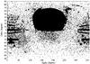 |
Fig. 4 Equatorial source positions of the LQAC-2 quasars. |
6.1. Mean density according to equatorial and galactic latitudes
We study here the sky coverage of the LQAC-2 with respect to the equatorial and galactic coordinates. In Fig. 4 we show the positioning of the sources in the equatorial system. We note that a very high proportion of sources (more than 70%) is located in a zone between α = 110° and α = 260° in right ascension and between δ = 0° and δ = 60° in declination, which only represents 18% of the whole celestial sphere. This explains the lack of homogeneity of the histograms for right ascension (Fig. 5) and in declination (Fig. 6). The two depletion zones α ≈ [60°−110°] and α ≈ [260°−310°] are clearly due to the vertical crossing of the Galactic plane. The deficiency of detections in the southern hemisphere, clearly visible in Figs. 4 and 6 comes from the poor exploration of large surveys involved in the compilation in this hemisphere, which contains 25% of the sample. The distribution of sources according to the Galactic longitude is rather homogenous (Fig. 7) whereas it is drastically lowered in the neighborhood of the galactic plane. The percentage of sources between l = −20° and l = +20° represents only 3% of the sample, although the corresponding ratio of the celestial sphere is 68.4%. Finally, we evaluate the variability of the mean density of quasars in unit of square degree in the LQAC-2 by constructing sectors in the celestial sphere, each of them delimited by two Galactic meridans separated by a Galactic longitude bin of 360°/41 252 = 0.008726° (41 252 representing the number of square degrees in the whole celestial sphere). Because the LQAC-2 contains 187 504 quasars, we can expect an average number of 4.54 quasars per square degree. The histogram giving the number of sources per square degree is presented in Fig. 9. The curve shows a typical Poisson distribution, as expected (see for instance Mignard 2008) for a set of uniformy and randomly distributed points. The large inhomogeneity of surface density already mentioned above does not affect this tendency noticeably.
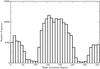 |
Fig. 5 Histogram of the number of sources in the LQAC-2 with respect to the right ascension. |
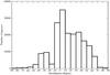 |
Fig. 6 Histogram of the number of sources of the LQAC-2 with respect to the declination. |
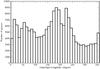 |
Fig. 7 Histogram of the number of sources of the LQAC-2 with respect to the Galactic longitude. |
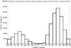 |
Fig. 8 Histogram of the number of sources of the LQAC-2 with respect to the Galactic latitude. |
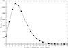 |
Fig. 9 Number of 1 square degree fields with respect to the number of sources in the LQAC-2. |
6.2. The “nearest neighbor” analysis
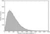 |
Fig. 10 Histogram of distance to the nearest neighbor for the whole LQAC-2 catalog. |
The theoretical foundations, as well as the basic laws that govern the presence of the nearest neighbor in small field astronomy whern considering that the sources (stars or quasars in the present case) have a uniform spatial distribution, can be found in a review by Mignard (2008). They are based on the fact that in the case of a uniform density, the actual number of sources to be found in a particular area S in a random drawing is given by a Poisson law. A complete analysis of the all-sky density of quasars in the LQAC-2, together with a statistical study of the closest neighbour angular distance following the equation above, will be the topic of our next paper. Here we are content with showing in Fig. 10 the histogram of the angular distance to the closest neighbor, which seems to clearly respect the Raighleigh distribution scheduled by theoretical assumptions (Mignard 2008). The curve peaks at roughly 210′′, that is to say 3.5′.
7. Description of the LQAC-2 data file
The LQAC-2 constructed in this paper gathers a total amount of 187 504 objects that can be characterized as quasars in the frame of a unified theory, including a certain number of AGNs (see Sect. 2). The morphological indexes enable one to understand in the best way wether we can identify these objects as point-like sources. In the following we explain the various items for each line of the catalog in details. Although the format is close to the LQAC in its first version, it contains more items as a number of identification, the coordinates given by the LQRF-2, and the morphological information. In the following we describe each item one by one, with the corresponding format.
7.1. Data and format
-
Column 1 gives the reference number of the quasar in the catalog,with the strategy explained in Sect. 5.2. Thisstrategy has the advantage of both proposing a rather simple namegiving directly the zone of the sky concerned and not changing thisname in the case of future updates of the LQAC.
-
Columns 2 and 3 are the α, δ coordinates given by the original catalog whose the flag comes first in alphabetic order (see two items below). This catalog a priori gives the best estimate in term of astrometric accuracy.
-
Columns 4 and 5 are the α, δ coordinates given by the LQRF-2.
-
Column 6 provides the letter codes (flags) indicating the presence of the quasar in one of the 13 catalogs from A to M as given by the nomenclature in Sect. 4.1. The advantage is to give the reader the name of the catalog in which the quasar is present.
-
Column 7 is a flag already present in the first version of the LQAC (Souchay et al. 2009) characterizing the objects that have a crossidentification angular distance ρ with a VV2010 counterpart larger than 2′′, and consequently are subject to doubtful crossidentification. A flag “ ⋆ ” stands for a quasar with 2″ < ρ < 5″ and Δz < 0.1, whereas a flag “!” stands for a quasar with 2″ < ρ < 5″ and Δz > 0.1. A flag denoted “x” stands for a quasar with ρ > 5″ and Δz < 0.1, whereas a flag denoted “?” stands for a quasar with ρ > 5″ and Δz > 0.1
-
Column 8 indicates with a flag “1” when the quasar has a very bad position in the original catalog.
-
Columns 9 to 15 give the visual apparent magnitudes listed by decreasing frequency, for the u, b, v, g, r, i, z bands respectively. The photometric systems in which these magnitudes have been measured are not homogoneous. This is, for instance, the case of the r band present both in the SDSS and the 2QZ catalogs. Therefore when a magnitude is available in two catalogs or more we privilegie the value given by the first flag in chronological order.
-
Columns 16 and 17 give the J and K infrared magnitudes coming from the cross-identification with the 2MASS catalog.
-
Columns 19 to 23 give the radio flux at 1.4 GHz (20 cm), 2.3 GHz (13 cm), 5.0 GHz (6 cm), 8.4 GHz (3.6 cm), and 24 GHz (1.2 cm), respectively, found in the radio catalogs (flags A to D)
-
Columns 24 and 25 give the redshift value z of each quasar and the reference number of the catalog from which it was taken, identical to that from the VV2010 catalog. A specific file provided with the LQAC-2 indicates the correspondences between the catalog reference number and the catalog name.
-
Columns 26 to 31 gather the data used for estimating the absolute magnitude (see Sect. 4.4). The first two columns are the value of the bolometric distance and of the galactic extinction. Columns 28 and 29 stand for the K- correction for b and i bands. The last two Cols. 30 and 31 are the values of the absolute magnitudes Mb and Mi in b and i bands, calculated from the formula detailed in Sect. 4.4.
-
Columns 32 to 40 provide us with the morphological indexes whose the determination has been explained in full detail in Sect. 5.4. They concern the B (Cols. 32 to 34), R (Cols. 35 to 37), I (Cols. 38 to 40) bands with three indexes each, the first one characterizing the skewness, the second one the roundness, and the last the normalness.
In Fig. 11 we present a sample of a few lines of the LQAC-2 catalog for information.
7.2. Access to the LQAC-2 data and update
The LQAC-2 extended catalog has been stored in the VOTable format compatible with Astronomy VO Data Format and VO tools. This catalog is more complete than the ASCII version. The LQAC-2 in ASCII and VOtable formats and all annex information are available at the ICRS Product Center website at the Paris Observatory (http://hpiers.obspm.fr/icrs-pc) or by anonymous ftp to ftp://syrte.obspm.fr/pub/LQAC-2
8. Conclusion
This paper presents the second release of the Large Quasar Astrometric Catalogue, called LQAC-2, which is a compilation of all the recorded quasars. It is an improved version of the first release (Souchay et al. 2009). It contains 187 504 objects, which is a 65% increase over the 113 666 quasars in the first LQAC catalog. Moreover, it includes new features that considerably extends the information for the objects.
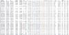 |
Fig. 11 Presentation of a sample of few lines of the LQAC-2 catalog. |
These are: adopting of a LQAC classification number based on the celestial coordinates; adding of the celestial coordinates of the quasars in the LQRF (Andrei et al. 2009), which are generally signficantly more accurate than the celestial coordinates found in the original catalogs; determining three morphological indexes (skewness, roundness, normalness) for each of the three bands B, R, and I. The quasars in the LQAC-2 come principally from a set of nine leading quasars catalogs chosen for their optimal accuracy (as the ICRF2) or their density (as the SDSS). In addition, 22 440 objects not included in these nine catalogs are picked up from the Véron-Cetty & Véron (2010) catalog, in order to insure a complete sample. To provide some missing information concerning the photometry (apparent magnitudes of the quasars), we used the GSC2.3 (Lasker et al. 2008), B1.0 (Monet et al. 2003), and 2MASS (Cutri et al. 2003) all-sky surveys. We think that the LQAC-2 presented in this paper will be useful for the astronomical community, for listing all the recorded quasars with emphasis on their astrometric accuracy. Moreover it should give birth to interesting statistical studies of several topics: analysis of the spatial density and of the correlation between parameters (redshift, absolute magnitudes, colors etc.), preparation for the Gaia space mission, comparison of the radio and optical positions of radio stars (Andrei et al. 1995) etc. It should be fully used for determining of close approachs between quasars and moving objects such as asteroids and planets (Souchay et al. 2007; Nedelcu et al. 2010) or comparisons between catalogs (Souchay et al. 2008).
Acknowledgments
The authors acknowledge the use of the Digitized Sky Surveys produced at the Space Telescope Science Institute under U.S. Government grant NAG W-2166. The images of these surveys are based on photographic data obtained using the Oschin Schmidt Telescope on Palomar Mountain and the UK Schmidt Telescope. The plates were processed into the present compressed digital form with the permission of these institutions. Funding for SDSS-III has been provided by the Alfred P. Sloan Fundation, the participating Institutions, the National Science Fundation, and the U.S. Department of Energy. A.H.A. thanks CNPq grant PQ-307126/2006-0.and the PARSEC International Incoming Fellowship within the Marie Curie 7th European Community Framework Programme. This research has made full use of the Virtual Observatory tools such as Aladin and Vizier (Strasbourg, France). We also used Topcat and Stilts tools from Mark Mayer, Astrophysics Group, Physics Department, Bristol University.
References
- Abazajian, K., Adelman-McCarthy, J. K., Agueros, M. A., et al. 2009, ApJS, 182, 543 [NASA ADS] [CrossRef] [Google Scholar]
- Adelman-McCarthy, J. K., Agüeros, M. A., Allam, S. S., et al. 2007, ApJS, 172, 634 [NASA ADS] [CrossRef] [Google Scholar]
- Aihara, H., Prieto, C. A., An, D., et al. 2011, ApJS, 193, 29 [NASA ADS] [CrossRef] [Google Scholar]
- Andrei, A. H., Jilinski, E. G., & Puliaev, S. P. 1995, AJ, 109, 428 [NASA ADS] [CrossRef] [Google Scholar]
- Andrei, A. H., Souchay, J., Zacharias, N., et al. 2009, A&A, 505, 385 [NASA ADS] [CrossRef] [EDP Sciences] [MathSciNet] [Google Scholar]
- Boboltz, D. A., Gaume, R. A., Fey, A. L., et al. 2010, BAAS, 42, 512 [NASA ADS] [Google Scholar]
- Claussen, M. 2006, VLA Calibrator Manual [Google Scholar]
- Croom, S. M., Smith, R. J., Boyle, B. J., et al. 2004, MNRAS, 349, 1397 [NASA ADS] [CrossRef] [Google Scholar]
- Cutri, R. M., Skrutskie, M. F., Van Dyk, S., et al. 2003, IPAC/California Institute of Technology [Google Scholar]
- da Angela, J., Shanks, T., Croom, S. M., et al. 2008, MNRAS, 383, 565 [NASA ADS] [CrossRef] [Google Scholar]
- De Veny, J. B., Osborn, W. H., & Janes, K. 1971, PASP, 83, 611 [NASA ADS] [CrossRef] [Google Scholar]
- Falomo, R., Kotilainen, J. K., & Treves, A. 2001, ApJ, 547, 124 [NASA ADS] [CrossRef] [Google Scholar]
- Fan, X., Strauss, M. A., Schneider, D. P., et al. 1999, AJ, 118, 1 [NASA ADS] [CrossRef] [Google Scholar]
- Fey, A. L., Boboltz, D. A., Gaume, R. A., Eubanks, T. M., & Johnston, K. J. 2001, AJ, 121, 1741 [NASA ADS] [CrossRef] [Google Scholar]
- Fomalont, E., Petrov, L., Mc Millan, D. S., Gordon, D., & Ma, C. 2003, AJ, 126, 2562 [NASA ADS] [CrossRef] [Google Scholar]
- Fukugita, M., Ichikawa, T., Gunn, J. E., et al. 1996, AJ, 111, 1748 [NASA ADS] [CrossRef] [Google Scholar]
- Gregg, M. D., Becker, R. H., White, R. L., et al. AJ, 112, 407 [Google Scholar]
- Hewitt, A., & Burbridge, G. 1993, ApJSS, 87, 2, 451 [CrossRef] [Google Scholar]
- Hogg, D. W., Pahre, M. A., Adelberger, K. L., et al. 2000, ApJS, 127, 1 [NASA ADS] [CrossRef] [Google Scholar]
- Komatsu, E., Smith, K. M., Dunkley, J., et al. 2011, ApJS, 912, 18 [NASA ADS] [CrossRef] [Google Scholar]
- Lasker, B., Lattanzi, M. G., Mc Lean, B. J., et al. 2008, AJ, 136, 735L [NASA ADS] [CrossRef] [Google Scholar]
- Ma, C., Arias, E. F., Eubanks, T. M., et al. 1998, AJ, 116, 516 [NASA ADS] [CrossRef] [Google Scholar]
- Ma, C., Arias, E. F., Bianco, G., et al. 2009, IERS Technical Note No. 35 [Google Scholar]
- Mignard, F. 2008, GAIA-C4-Technical Note-OCA-FM-035-1 [Google Scholar]
- Monet, D. G., Levine, S. E. C. B., Ables, H. D., et al. 2003, AJ, 125, 984 [NASA ADS] [CrossRef] [Google Scholar]
- Nedelcu, D. A., Birlan, M., Souchay, J., et al. 2010, A&A, 509, A27 [NASA ADS] [CrossRef] [EDP Sciences] [Google Scholar]
- Petrov, L., Kovalev, Y. Y., Fomalont, E., & Gordon, D. 2008, AJ, 136, 580 [NASA ADS] [CrossRef] [Google Scholar]
- Richards, G. T., Croom, S. M., Anderson, S. F., et al. 2005, MNRAS, 360, 839 [NASA ADS] [CrossRef] [Google Scholar]
- Richards, G. T., Lacy, M., Storrie-Lombardi, L. J., et al. 2006, AJ, 131, 2766 [NASA ADS] [CrossRef] [Google Scholar]
- Sakata, M., Yoshii, K., Koshida, A., et al. 2010, ApJ, 711, 461 [NASA ADS] [CrossRef] [Google Scholar]
- Schlegel, D. J., Finkbeiner, D. P., & Davis, M. 1998, ApJ, 500, 525 [NASA ADS] [CrossRef] [Google Scholar]
- Schneider, D. P., Richards, G. T., Hall, P. B., et al. 2010, AJ, 139, 2360 [NASA ADS] [CrossRef] [Google Scholar]
- SDSS DR5 2006, The SDSS Data Release 5, Description and data available at: http://www.sdss.org/dr5 [Google Scholar]
- Souchay, J., Le Poncin-Lafitte, C., & Andrei, A. H. 2007, A&A, 471, 335 [NASA ADS] [CrossRef] [EDP Sciences] [Google Scholar]
- Souchay, J., Lambert, S. B., Andrei, A. H., et al. 2008, A&A, 485, 299 [NASA ADS] [CrossRef] [EDP Sciences] [Google Scholar]
- Souchay, J., Andrei, A. H., Barache, C., et al. 2009, A&A, 494, 815 [Google Scholar]
- Véron-Cetty, M. P., & Véron, P. 2006, A&A, 455, 773 [NASA ADS] [CrossRef] [EDP Sciences] [Google Scholar]
- Véron-Cetty, M. P., & Véron, P. 2010, A&A, 518, A10 [NASA ADS] [CrossRef] [EDP Sciences] [Google Scholar]
- Zacharias, N., Urban, S. E., Zacharias, M. I., et al. 2004, AJ, 127, 3043 [NASA ADS] [CrossRef] [Google Scholar]
All Tables
Characteristics of the catalogs participating to our compilation of quasars both for the LQAC-2 and the LQAC.
Photometry and redshift information from each optical catalog of the LQAC compilation.
Infrared photometry and radio flux informations available according to corresponding catalogs of the LQAC compilation.
Comparison of the number of entries for each data item between the VV2010 catalog, the compilation of the catalogs A-L and the final LQAC-2 catalog.
Number of morphological indexes and quantity of objects off 2σ from the local mean stellar PSF.
All Figures
|
Fig. 1 Binned distribution of the morphological index SHARP. The color codes stand for the respective DSS plates. |
| In the text | |
|
Fig. 2 Binned distribution of the morphological index SROUND. The color codes stand for the respective DSS plates. |
| In the text | |
|
Fig. 3 Binned distribution of the morphological index GROUND. The color codes stand for the respective DSS plates. |
| In the text | |
|
Fig. 4 Equatorial source positions of the LQAC-2 quasars. |
| In the text | |
|
Fig. 5 Histogram of the number of sources in the LQAC-2 with respect to the right ascension. |
| In the text | |
|
Fig. 6 Histogram of the number of sources of the LQAC-2 with respect to the declination. |
| In the text | |
|
Fig. 7 Histogram of the number of sources of the LQAC-2 with respect to the Galactic longitude. |
| In the text | |
|
Fig. 8 Histogram of the number of sources of the LQAC-2 with respect to the Galactic latitude. |
| In the text | |
|
Fig. 9 Number of 1 square degree fields with respect to the number of sources in the LQAC-2. |
| In the text | |
|
Fig. 10 Histogram of distance to the nearest neighbor for the whole LQAC-2 catalog. |
| In the text | |
|
Fig. 11 Presentation of a sample of few lines of the LQAC-2 catalog. |
| In the text | |
Current usage metrics show cumulative count of Article Views (full-text article views including HTML views, PDF and ePub downloads, according to the available data) and Abstracts Views on Vision4Press platform.
Data correspond to usage on the plateform after 2015. The current usage metrics is available 48-96 hours after online publication and is updated daily on week days.
Initial download of the metrics may take a while.