| Issue |
A&A
Volume 537, January 2012
|
|
|---|---|---|
| Article Number | A96 | |
| Number of page(s) | 8 | |
| Section | The Sun | |
| DOI | https://doi.org/10.1051/0004-6361/201117943 | |
| Published online | 25 January 2012 | |
Numerical simulations of magnetoacoustic oscillations in a gravitationally stratified solar corona⋆
1 Group of Astrophysics, Institute of Physics, UMCS, ul. Radziszewskiego 10, 20-031 Lublin, Poland
e-mail: This email address is being protected from spambots. You need JavaScript enabled to view it.
; This email address is being protected from spambots. You need JavaScript enabled to view it.
2 Space Research Institute, Austrian Academy of Sciences, Schmiedlstrasse 6, 8042 Graz, Austria
e-mail: This email address is being protected from spambots. You need JavaScript enabled to view it.
3 Abastumani Astrophysical Observatory at Ilia State University, University St. 2, Tbilisi, Georgia
Received: 24 August 2011
Accepted: 5 November 2011
Abstract
Aims. We consider magnetoacoustic oscillations in a gravitationally stratified solar corona, that are triggered by an initial pulse in the vertical component of velocity launched from various altitudes of the solar atmosphere.
Methods. We numerically solve two-dimensional magnetohydrodynamic equations for an ideal plasma to determine the spatial and temporal signatures of excited oscillations.
Results. Our numerical results reveal that few-min oscillations are effectively excited by the initial velocity pulses and that their waveperiods depend on the vertical location and amplitude of the pulse.
Conclusions. The building block of this scenario consists of a one-dimensional rebound shock model.
Key words: magnetohydrodynamics (MHD) / Sun: atmosphere / Sun: oscillations
Movies attached to Figs. 5 and 6 are available in electronic form at http://www.aanda.org
© ESO, 2012
1. Introduction
Waves and oscillations are seen in the solar corona. In particular, three- and five-minute oscillations are detected in coronal loops (e.g. De Moortel et al. 2000; 2002). Multi-wavelength observations of five-minute oscillations in loops were made by Marsh et al. (2003), and three- and five-minute oscillations associated with moving magnetic features were observed by Lin et al. (2006). The propagating upward slow magnetoacoustic waves with periods of about 5 min were detected in the transition region and coronal emission lines by Hinode/EIS at the footpoint of a coronal loop rooted at a plage (Wang et al. 2009).
It is apparent that the 5-min period corresponds to the main period of p-modes, which may be a potential explanation of the coronal oscillations. However, in the case of a gravitationally stratified isothermal atmosphere the dispersion relation for vertically propagating acoustic waves can be derived from the Klein-Gordon equation, which implies that the acoustic cut-off period, Pac, is shorter than 5 min (e.g. Lamb 1908; Roberts 2004). Since waves are able to propagate for wave periods shorter than Pac, we infer that the 5-min oscillations are unable to penetrate into the solar corona.
Bel & Leroy (1977) suggested that the cut-off frequency of the magnetic field-free atmosphere is lower when waves propagate with the angle to the vertical. McIntosh (2006) found the observational justification of the modification of the cut-off frequency along an inclined magnetic field (see Murawski & Zaqarashvili 2010 for recent numerical simulations of spicules). De Pontieu et al. (2004) proposed that as a result of a fall-off in the acoustic cut-off frequency p-modes may be channeled into the solar corona along inclined magnetic field lines. The oscillations may then be steepened into shocks producing spicules. De Pontieu et al. (2004) argued that the observed quasi 5-min period in spicule appearance is associated with the periodicity of p-modes. Zaqarashvili et al. (2010) proposed that 5-min oscillations in the solar corona originate in granules that they modeled by a vertical propagating wavefront in the vertical velocity component. However, Zaqarashvili et al. (2010) considered a simple one-dimensional (1D) problem of 5-min oscillations. The 1D case treats the acoustic waves only while the internal gravity waves are removed from the system. Therefore, there was a need to consider a two-dimensional (2D) scenario albeit in a hydrodynamic approximation in which both acoustic and internal gravity waves are present (Konkol & Murawski 2011).
The aim of this paper is to extend the 2D hydrodynamic model of Konkol & Murawski (2011), by adding magnetic fields and studying the influence of the initial velocity pulse location and its amplitude on the wave-periods of triggered oscillations. This paper is organized as follows. The numerical model is described in Sect. 2. The numerical results are presented and discussed in Sect. 3. This paper concludes with a short summary of the main results.
2. A numerical model
2.1. Magnetohydrodynamic equations
Our model system is assumed to be composed of a gravitationally stratified solar atmosphere that is described by the 2D ideal magnetohydrodynamic (MHD) equations: ![Mathematical equation: \begin{eqnarray} \label{eq:rho} &&{\partial\varrho\over \partial t}+\nabla\cdot \left(\varrho{\vec V}\right)=0,\\ \label{eq:rhoV} &&{\partial (\varrho {\vec V})\over\partial t}+ \nabla \cdot (\varrho{\vec V}{\vec V}-{\vec B}{\vec B}) + \nabla \cdot p_* = \rho {\vec g}, \\ \label{eq:E} &&{ \partial (\varrho E) \over \partial t } + \nabla \cdot [{\vec V}(\varrho E + p_*) - {\vec B}({\vec V} \cdot {\vec B})] = \varrho {\vec g} \cdot {\vec V}, \\ \label{eq:induct} &&{\partial{\vec B}\over\partial t} + \nabla \cdot({\vec V}{\vec B}-{\vec B}{\vec V}) = 0, \hspace{2.5mm} \nabla\cdot{\vec B} = 0,\\ \label{eq:CLAP} &&p = \frac{k_{\rm B}}{\hat m } \varrho T, \end{eqnarray}](/articles/aa/full_html/2012/01/aa17943-11/aa17943-11-eq3.png) with
with  (6)Here p∗ is the total (gas plus magnetic) pressure, ϱE is total (kinetic plus internal and magnetic) energy density, ϱϵ is internal energy density, ϱ is the mass density, V = [Vx,Vy,0] is the flow velocity, p is the gas pressure, g = [0, − g,0] is a constant gravity, B = [Bx,By,0] is the magnetic field that is normalized as
  where μ is the magnetic permeability, T is plasma temperature, γ = 5/3 is the adiabatic index, kB is Boltzman’s constant, and
  denotes the mean mass.
2.2. Initial configuration
2.2.1. The equilibrium
We assume that in equilibrium the solar atmosphere is a still (V = 0) environment with a gas pressure and a mass density given by  (7)where
  (8)is the pressure scale-height, and p0 denotes the gas pressure at the reference level that we set and hold fixed at y = yr = 10 Mm.
We adopt the temperature profile,  , for the solar atmosphere that was derived by Vernazza et al. (1981). This profile is displayed in Fig. 1. We note that
  attains a value of about 5700 K at the top of the photosphere, which corresponds to y = 0.5 Mm. At higher altitudes, falls off until it reaches its minimum of 4350 K at the altitude of y ≃ 0.95 Mm. Higher up increases gradually with height up to the transition region, which is located at y ≃ 2.7 Mm. Here experiences a sudden growth up to the coronal value of 1.5 MK at y = 10 Mm. After specifying using the equations in Eq. (7), we can obtain mass density and gas pressure profiles as seen in Fig. 2. Both p(y) and ϱ(y) experience a sudden fall off from photosphere to coronal values at the transition region.
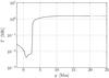 |
Fig. 1 Equilibrium temperature T (in mega Kelvins) (vs.) height y (in Mm) for the solar atmosphere. |
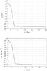 |
Fig. 2 Equilibrium profiles of gas pressure p (top) and gas density ϱ (bottom). |
The evolution of small-amplitude acoustic waves can be described by the Klein-Gordon equation (Roberts 2004)  (9)where
  This equation describes vertically propagating acoustic waves in a gravitationlly stratified atmosphere. For the isothermal atmosphere, cs = const. and Λ = const. The exact dispersion relation can then be derived (Roberts 2004). For slowly varying cs(y), we can derive an approximate dispersion relation such as
 where ω is the wave frequency and the cut-off frequency Ωac is given as
  (12)The acoustic cut-off period, Pac = 2π/Ωac, in the low chromosphere is about 200 s and then sharply lengthens up to the transition region, where it reaches coronal values such as at y = 10 Mm Pac = 3.5 × 10³ s. We note that Eq. (12) can be obtained from the linear analysis, while the nonlinear description can alter the oscillation period of a wake (Zaqarashvili et al. 2010).
We adopt a current-free magnetic field  (13)where
  (14)Here A denotes a magnetic flux function such as
  (15)where s is a strength of the magnetic moment that is located at ax = 0 Mm and ay = −15 Mm. We choose s by requiring that at the reference point (0,10) Mm the Alfvén speed is
  (16)and sound speed
  (17)satisfy the following constraint: cA(0,10) = 10cs(10). This constraint depends on the typical conditions in the solar corona, where cs = 0.1 Mm s-1 and cA = 1 Mm s-1. Magnetic field vectors given by Eq. (14) are displayed in Fig. 3.
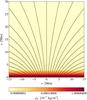 |
Fig. 3 Equilibrium magnetic field vectors (fieldlines). |
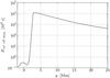 |
Fig. 4 Magnetic cut-off wave period (in units of 103 s) vs. height y (in Mm). |
Taking magnetic effects into account, Roberts (2006) derived the magnetic cut-off frequency  (18)where
  denotes the buoyancy or Brunt-Väisälä frequency
  (19)and
 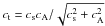 . Figure 4 shows the magnetic cut-off period Pm = 2π/Ωm. We note that for y = 0 Mm, Pm attains a value of about 300 s. At greater heights it falls off to about 190 s at y ≃ 0.8 Mm and then it increases abruptly at the transition region, reaching a magnitude of about 107 s. At higher altitudes, Pm declines far more slowly with height. By comparing Pm and Pac, we can infer that they are close in a weakly magnetized plasma (solar photosphere) and differ much in the solar corona, where the magnetic pressure is higher than the gas pressure. Since waves propagate when their waveperiods are shorter than a cut-off waveperiod, we conclude that a magnetic field allows longer waveperiod waves to propagate into the corona than into the magnetic-free medium.
 |
Fig. 5 Total velocity |V(x,y)| (colour maps) and velocity vectors (arrows) profiles at t = 180 s (top-left), 250 s (top-right), 320 s (bottom-left), and 390 s (bottom-right) for Av = 2 km s-1 and y0 = 0.7 Mm. A movie showing the temporal evolution is available in the online edition. |
2.2.2. Perturbations
We excite waves in the aforementioned solar atmosphere by launching initially, at t = 0 s, the impulse in a vertical component of velocity Vy, i.e. ![Mathematical equation: \begin{equation} \label{eq:perturb} V_{\rm y}(x,y,t=0) = A_{\rm v}\exp\left[-\frac{x^2 + (y-y_{\rm 0})^2}{w^2} \right]\cdot \end{equation}](/articles/aa/full_html/2012/01/aa17943-11/aa17943-11-eq85.png) (20)Here Av is the amplitude of the initial Gaussian pulse, y0 its initial position, and w its width. We set and hold fixed w = 0.1 Mm but allow Vy and y0 to vary.
(20)Here Av is the amplitude of the initial Gaussian pulse, y0 its initial position, and w its width. We set and hold fixed w = 0.1 Mm but allow Vy and y0 to vary.
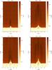 |
Fig. 6 Plasma temperature T (colour maps) and velocity vectors (arrows) profiles at t = 180 s, 250 s, 320 s, and 390 s, for Av = 2 km s-1 and y0 = 0.7 Mm. A movie showing the temporal evolution is available in the online edition. |
3. Numerical results
We solve Eqs. (1)−(5) numerically, using the code FLASH (Dubey et al. 2009), which implements a second-order unsplit Godunov solver and Adaptive Mesh Refinement (AMR). We set the simulation box over a span of 22 Mm in the x- and y-directions. At all boundaries, we fix all plasma quantities to their equilibrium values. In our studies, we use the AMR grid with a minimum (maximum) level of refinement blocks set to 3 (10). The refinement strategy is based on controlling numerical errors in a gradient of temperature. These settings provide steep spatial profiles of excellent resolution, which significantly reduce the numerical diffusion within the simulation region.
Figure 5 illustrates the spatial profiles of the total velocity |V|, and velocity vectors at t = 180 s, t = 250 s, t = 320 s, and t = 390 s for the initial pulse amplitude Av = 2 km s-1. The initial pulse separates in its usual way into counter-propagating waves, which can be clearly seen at t = 180 s (top-left). The waves propagating upwards grow in terms of their amplitudes as a result of the rapid decrease in the mass density of the chromosphere (Zaqarashvili et al. 2010). As a consequence of this, a shock results. At t = 250 s, the leading shock reached the height of y = 18 Mm (top-right), whereas the secondary shock had already started to propagate upwards, and is located around the point (x = 0,y = 3) Mm. At a later moment of time, at t = 320 s, this secondary shock penetrates the solar corona, reaching the altitude y = 8 Mm (bottom-left). At t = 390 s, the secondary shock is at y ≃ 18 Mm and the third shock evolves upwards around the point (x = 0,y = 2) Mm (bottom-right).
Figure 6 shows the spatial profiles of the temperature T (in logarithmic scale) and velocity vectors at t = 180 s, t = 250 s, t = 320 s and t = 390 s for the initial pulse amplitude Av = 2 km s-1, and y0 = 0.5 Mm. The cold plasma of the photosphere and chromosphere is pushed up by the underpressure residing behind the shock (top-left). The pressure gradient force lifts the cold material towards the solar corona (Murawski & Zaqarashvili 2010). The secondary shock can be clearly seen at t = 250 s (top-right). Later on, at t = 320 s, the helmet-shape structure occurs as a result of a complex interaction between the secondary and leading oscillations of the transition region (bottom-left). This shape becomes conic-like at t = 390 s (bottom-right).
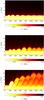 |
Fig. 7 Vertical slices of temperature along x = 0, for Av = 2 km s-1, y0 = 1.50 Mm (top), y0 = 1.00 Mm (middle), and y0 = 0.50 Mm (bottom). |
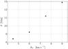 |
Fig. 8 Amplitude of oscillations of the transition region vs. initial pulse amplitude, Av for y0 = 0.6 Mm. |
Figure 7 displays the spatial evolution of temperature in the vertical direction, for x = 0, for pulses launched at y0 = 1.50 Mm (top), 1.00 Mm (middle), and 0.50 Mm (bottom). All panels reveal oscillations of the transition region caused by the initial velocity pulse. In addition, we illustrate that the deeper launched (smaller y0) pulse generates larger amplitude disturbances. In the lower regions, the plasma is much denser so the same pulse has more kinetic energy and momentum. A more energetic pulse is obviously able to trigger larger amplitude oscillations (Fig. 8).
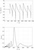 |
Fig. 9 Time-signatures of Vy (in units of km s-1) collected at (x = 0,y = 25) Mm and its Fourier power spectrum for Av = 2 km s-1 and y0 = 0.7 Mm. |
Figure 9 displays time-signatures of Vy (upper panel) and its Fourier power spectrum (lower panel), for the case of Fig. 5. This velocity is collected in time at the detection point (x = 0,y = 20) Mm. The arrival of the leading shock front to the detection point occurs at t ≃ 300 s. The secondary shock reaches the detection point at t ≃ 430 s. This shock results from the nonlinear wake, which lags behind. This Fourier power spectrum reveals that most of the power is associated with the waveperiod P ≃ 210 s, with lower contributions from shorter values of P. These contributions are insignificant from the observational point of view because at low power they may be hidden by the background noise in the real medium. We note that in the linear approximation the wake oscillates with the acoustic cut-off frequency of Eq. (18), which for y0 = 0.7 Mm leads to P ≃ 180 s.
Figure 10 shows a plot of the oscillation waveperiod P vs. pulse height y0. For the pulses closer to the transition region, the oscillation period is close to the local Pm (Fig. 4). However, for lower values of y0 (owing to higher kinetic energy), the resulting periods differ from those predicted by Eq. (12).
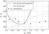 |
Fig. 10 Waveperiod P vs. pulse location y0 for pulse amplitude Av = 2 km s-1. |
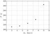 |
Fig. 11 Waveperiod P vs. pulse amplitude Av for y0 = 0.5 Mm. |
Figure 11 displays a plot of oscillation period P vs. pulse amplitude Av for y0 = 0.5 Mm. The period increases with the amplitude of the pulse and may reach a value of about 5 min for Av = 9 km s-1. The presence of a magnetic field results in more regular oscillations, owing to the lack of detected vortices in the magnetic-free medium (Konkol & Murawski 2011). In addition, a strong magnetic field below the transition region (the pulse is launched above the magnetic pole) allows us to compare our numerical results with the cut-off frequency of Eq. (12) derived from the simple 1D model provided by the Klein-Gordon equation (Roberts 2006).
4. Discussion and conclusions
The way in which disturbances in the solar corona are excited remains still an unanswered question. The disturbances often have a quasi-periodic behavior with a period that is similar to the oscillation spectrum of the photosphere/chromosphere, i.e. 3−5 min. These propagating features are assumed to be slow magnetoacoustic waves. However, some Hinode observations (De Pontieu & McIntosh 2010) have questioned this hypothesis, suggesting that the propagating disturbances are periodic upflows rather than waves. The correct solution should be a topic of further discussion.
The coincidence of the observed periods of coronal and photospheric oscillations logically leads to the idea that the photospheric oscillations leak into the corona along inclined magnetic fields (De Pontieu et al. 2005; Erdélyi et al. 2007; Fedun et al. 2009). However, Murawski and Zaqarashvili (2010) and Zaqarashvili et al. (2011) suggested that the observed periodicity in the solar corona is caused by quasi-periodic rebound shocks, originating from nonlinear wakes in the stratified atmosphere. Here we have developed the same idea and solved the ideal MHD equations in the case of a realistic temperature profile.
Our results show that the propagation of a velocity pulse in the stratified atmosphere leads to the nonlinear wake behind, which results in quasi-periodic shocks. These shocks penetrate into the corona and may cause the observed quasi-periodic variations in coronal line intensities. The interval between consecutive shocks, which coincides with the observed oscillation period, is within the range of cut-off periods associated with slow magnetoacoustic waves in the solar atmosphere. However, the resulting period is not equal strictly to the cut-off period, but it depends on the amplitude of initial pulse and the height from which the initial pulse was launched; a stronger amplitude pulse leads to a longer periodicity and a wave period that is slightly longer for the pulses launched below the temperature minimum.
We note that our simulations do not include non-adiabatic processes, such as thermal conduction and radiation. These processes may be important in the hot solar corona, but their inclusion would probably not significantly change the overall scenario as the periodicity is determined by the conditions in the lower cooler regions of the solar atmosphere. Nevertheless, their inclusion in numerical simulations would be desirable in future studies.
Online material
Movie 1 Access Supplementary Material
Movie 2 Access Supplementary Material
Acknowledgments
The work of T.Z. was supported by the Austrian Fonds zur Förderung der wissenschaftlichen Forschung (project P21197-N16) and the Georgian National Science Foundation (under grant GNSF/ST09/4-310). The software used in this work was in part developed by the DOE-supported ASC/Alliance Center for Astrophysical Thermonuclear Flashes at the University of Chicago. This work has been supported by a Marie Curie International Research Staff Exchange Scheme Fellowship within the 7th European Community Framework Program (P.K. and K.M.).
References
- Bel, N., & Leroy, B. 1977, A&A, 55, 239 [NASA ADS] [Google Scholar]
- De Moortel, I., Ireland, J., & Walsh, R. W. 2000, A&A, 355, L23 [NASA ADS] [Google Scholar]
- De Moortel, I., Ireland, J., Hood, A. W., & Walsh, R. W. 2002, A&A, 387, L13 [NASA ADS] [CrossRef] [EDP Sciences] [Google Scholar]
- De Pontieu, B., & McIntosh, S. W. 2010, ApJ, 722, 1013 [NASA ADS] [CrossRef] [Google Scholar]
- De Pontieu, B., Erdélyi, R., & James, S. P. 2004, Nature, 430, 536 [NASA ADS] [CrossRef] [PubMed] [Google Scholar]
- De Pontieu, B., Erdélyi, R., & De Moortel, I. 2005, ApJ, 624, L61 [NASA ADS] [CrossRef] [Google Scholar]
- Dubey, A., Antypas, K., Ganapathy, M. K., & Reid, L. B. 2009, Parallel Computing, ed. K. Riley, D. Sheeler, A. Siegel, & K. Weide, 35 [Google Scholar]
- Erdélyi, R., Malins, C., Tóth, G., & de Pontieu, B. 2007, A&A, 467, 1299 [NASA ADS] [CrossRef] [EDP Sciences] [Google Scholar]
- Fedun, V., Erdélyi, R., & Shelyag, S. 2009, Sol. Phys., 258, 219 [NASA ADS] [CrossRef] [Google Scholar]
- Hollweg, J. V. 1982, ApJ, 257, 345 [NASA ADS] [CrossRef] [Google Scholar]
- Konkol, P., & Murawski, K. 2011, Acta Phys. Polon., submitted [Google Scholar]
- Lin, C. H., Banerjee, D., Doyle, J. G., & O’Shea, E. 2005, A&A, 444, 585 [NASA ADS] [CrossRef] [EDP Sciences] [Google Scholar]
- Lin, C. H., Banerjee, D., O’Shea, E., & Doyle, J. G. 2006, A&A, 460, 597 [NASA ADS] [CrossRef] [EDP Sciences] [Google Scholar]
- Lamb, H. 1908, Proc. London Math. Soc., 7, 122 [Google Scholar]
- Marsh, M. S., Walsh, R. W., De Moortel, I., & Ireland, J. 2003, A&A, 404, L37 [NASA ADS] [CrossRef] [EDP Sciences] [Google Scholar]
- McIntosh, S. W., & Jefferies, S. W. 2006, ApJ, 647, L77 [NASA ADS] [CrossRef] [Google Scholar]
- Murawski, K., & Zaqarashvili, T. 2010, A&A, 519, A8 [NASA ADS] [CrossRef] [EDP Sciences] [Google Scholar]
- Priest, E. R. 1982, Solar Magnetohydrodynamics (Dordrecht: D. Reidel) [Google Scholar]
- Roberts, B. 2004, In Proc. SOHO 13 Waves, Oscillations and Small-Scale Transient Events in the Solar Atmosphere: A Joint View from SOHO and TRACE, Palma de Mallorca, Spain, ESA SP-547, 1 [Google Scholar]
- Roberts, B. 2006, Phil. Trans. R. Soc. A, 364, 447 [CrossRef] [Google Scholar]
- Srivastava, A. K., Kuridze, D., Zaqarashvili, T. V., & Dwivedi, B. N. 2008, A&A, 481, L95 [NASA ADS] [CrossRef] [EDP Sciences] [Google Scholar]
- Tanenbaum, A. S., Wilcox, J. M., Franzier, E. N., & Howard, R. 1969, Sol. Phys., 9, 328 [NASA ADS] [CrossRef] [Google Scholar]
- Vernazza, J. E., Avrett, E. H., & Loeser, R. 1981, ApJ, 45, 635 [NASA ADS] [CrossRef] [Google Scholar]
- Wang, T. J., Ofman, L., & Davila, J. M. 2009, ApJ, 696, 1448 [NASA ADS] [CrossRef] [Google Scholar]
- Zaqarashvili, T. V., Murawski, K., Khodachenko, M. K., & Lee, D. 2011, A&A, 529, A85 [NASA ADS] [CrossRef] [EDP Sciences] [Google Scholar]
All Figures
|
Fig. 1 Equilibrium temperature T (in mega Kelvins) (vs.) height y (in Mm) for the solar atmosphere. |
| In the text | |
|
Fig. 2 Equilibrium profiles of gas pressure p (top) and gas density ϱ (bottom). |
| In the text | |
|
Fig. 3 Equilibrium magnetic field vectors (fieldlines). |
| In the text | |
|
Fig. 4 Magnetic cut-off wave period (in units of 103 s) vs. height y (in Mm). |
| In the text | |
|
Fig. 5 Total velocity |V(x,y)| (colour maps) and velocity vectors (arrows) profiles at t = 180 s (top-left), 250 s (top-right), 320 s (bottom-left), and 390 s (bottom-right) for Av = 2 km s-1 and y0 = 0.7 Mm. A movie showing the temporal evolution is available in the online edition. |
| In the text | |
|
Fig. 6 Plasma temperature T (colour maps) and velocity vectors (arrows) profiles at t = 180 s, 250 s, 320 s, and 390 s, for Av = 2 km s-1 and y0 = 0.7 Mm. A movie showing the temporal evolution is available in the online edition. |
| In the text | |
|
Fig. 7 Vertical slices of temperature along x = 0, for Av = 2 km s-1, y0 = 1.50 Mm (top), y0 = 1.00 Mm (middle), and y0 = 0.50 Mm (bottom). |
| In the text | |
|
Fig. 8 Amplitude of oscillations of the transition region vs. initial pulse amplitude, Av for y0 = 0.6 Mm. |
| In the text | |
|
Fig. 9 Time-signatures of Vy (in units of km s-1) collected at (x = 0,y = 25) Mm and its Fourier power spectrum for Av = 2 km s-1 and y0 = 0.7 Mm. |
| In the text | |
|
Fig. 10 Waveperiod P vs. pulse location y0 for pulse amplitude Av = 2 km s-1. |
| In the text | |
|
Fig. 11 Waveperiod P vs. pulse amplitude Av for y0 = 0.5 Mm. |
| In the text | |
Current usage metrics show cumulative count of Article Views (full-text article views including HTML views, PDF and ePub downloads, according to the available data) and Abstracts Views on Vision4Press platform.
Data correspond to usage on the plateform after 2015. The current usage metrics is available 48-96 hours after online publication and is updated daily on week days.
Initial download of the metrics may take a while.