| Issue |
A&A
Volume 537, January 2012
|
|
|---|---|---|
| Article Number | A102 | |
| Number of page(s) | 13 | |
| Section | Astrophysical processes | |
| DOI | https://doi.org/10.1051/0004-6361/201117700 | |
| Published online | 16 January 2012 | |
Enhanced H2O formation through dust grain chemistry in X-ray exposed environments
1 Leiden Observatory, Leiden University, PO Box 9513, 2300 RA Leiden, The Netherlands
2 Kapteyn Astronomical Institute, PO Box 800, 9700 AV Groningen, The Netherlands
e-mail: meijerink@astro.rug.nl
Received: 14 July 2011
Accepted: 6 November 2011
Context. The ultraluminous infrared galaxy Mrk 231, which shows signs of both black hole accretion and star formation, exhibits very strong water rotational lines between λ = 200−670 μm, comparable to the strength of the CO rotational lines. High-redshift quasars also show similar CO and H2O line properties, while starburst galaxies, such as M 82, lack these very strong H2O lines in the same wavelength range, but do show strong CO lines.
Aims. We explore the possibility of enhancing the gas phase H2O abundance in X-ray exposed environments, using bare interstellar carbonaceous dust grains as a catalyst. Cloud-cloud collisions cause C and J shocks, and strip the grains of their ice layers. The internal UV field created by X-rays from the accreting black hole does not allow reforming the ice.
Methods. We determined the formation rates of both OH and H2O on dust grains, with temperatures Tdust = 10−60 K, using both Monte Carlo and rate equation method simulations. The acquired formation rates were added to our X-ray chemistry code, which allowed us to calculate the thermal and chemical structure of the interstellar medium near an active galactic nucleus.
Results. We derive analytic expressions for the formation of OH and H2O on bare dust grains as a catalyst. Oxygen atoms arriving on the dust are released into the gas phase in the form of OH and H2O. The efficiencies of this conversion due to the chemistry occurring on dust are near 30 percent for oxygen converted into OH and 60 percent for oxygen converted into H2O between Tdust = 15−40 K. At higher temperatures, the efficiencies decline rapidly. When the gas is mostly atomic, molecule formation on dust is dominant over the gas-phase route, which is then quenched by the low H2 abundance. Here, it is possible to enhance the warm (T > 200 K) water abundance by an order of magnitude in X-ray exposed environments. This helps explain the observed bright water lines in nearby and high-redshift ULIRGs and quasars.
Key words: astrochemistry / ISM: abundances / galaxies: active / dust, extinction / galaxies: ISM / galaxies: starburst
© ESO, 2012
1. Introduction
Warm molecular gas (T > 100 K) cools mainly through CO, H2O, and H2 ro-vibrational transitions (Neufeld & Kaufman 1993; Neufeld et al. 1995). The ground state lines of CO, up to J = 6−5, are extensively studied from the ground in many galaxies (see, e.g., Papadopoulos et al. 2010) up to a redshift z ~ 0.04. Unfortunately, the atmosphere makes it impossible to study CO transitions with J > 8 and H2O rotational lines. It is these lines, however, that trace the warm molecular gas. Moreover, these lines are sensitive to extreme UV irradiation from star formation and X-rays due to supermassive black-hole accretion. Some high-J CO lines have been observed in bright galactic objects such as the Orion Bar and Sagittarius A (cf. Hollenbach & Tielens 1999), and the Class 0 object L1448-mm (Nisini et al. 1999). It is only recently that significant progress has been made in the study of the warm molecular interstellar medium (ISM) in nearby galaxies. Both high-J CO and rotational water lines have been observed abundantly after the launch of the Herschel Space Observatory, that operates between wavelengths λ = 55−672 μm. The successful HerCULES open-time key program has observed 29 close (U)LIRGs with both SPIRE and PACS instruments, revealing CO lines up CO J = 14−13 (while current follow-up PACS observations might detect even higher transition) and H2O lines in Mrk 231 that have comparable strengths (van der Werf et al. 2010; González-Alfonso et al. 2010). These CO and H2O lines are at least in part produced in regions of the galaxy exposed to X-rays, so-called XDRs (Maloney et al. 1996; Meijerink & Spaans 2005), but emission produced through shock excitation may also contribute, as observed for OH in Mrk 231 (Fischer et al. 2010). Moreover, Herschel-PACS also detected a lot of high-J CO lines, as well as H2O and OH in embedded objects, such as DK Chamaeleontis (van Kempen et al. 2010) and in disk atmospheres, e.g., HD 100546 (Sturm et al. 2010), where X-rays also affect the chemical-thermal structure.
Understanding the excitation and chemistry of these important molecules is therefore key to studying the dominant physical processes in the ISM and star formation. CO is a linear molecule, and the radiation transfer models allow calculating far-infrared to millimeter spectra relatively easily for a given physical structure. Models predicting CO emission, where both the thermal-chemical structure and radiation transfer are calculated simultaneously, have more problems reaching agreement. The case for H2O is even worse, thanks to its complex nature. High critical densities ncrit > 108 − 1010 cm-3 in combination with high opacities, infrared-pumping, and maser activity, make an excitation calculation extremely challenging. Also, the excitation state in which water enters the gas phase after desorption or evaporation from a dust grain is very uncertain. A first guess would be to divide the excess energy over the levels using equipartion, hence 1/3 translational, 1/3 rotational, and 1/3 vibrational excitation, with a Boltzmann distribution for the sub-levels.
The formation of molecular hydrogen, H2, in the ISM has been a longstanding problem. At extremely low metallicities, when no dust is present, H2 forms either through the H− route (H − + H → H2 + e-1; Glover 2003; Launay et al. 1991) or through a three-body reaction (H + H + H → H2 + H). The three-body reaction dominates at very high densities (n > 109 cm-3; Galli & Palla 1998). For normal ISM conditions, H2 is predominantly formed on dust grains, and much progress has been made over the past two decades, both experimentially and theoretically, in understanding this (much faster) formation of H2 on the surfaces of grains (Pirronello et al. 1999; Katz et al. 1999; Cazaux & Tielens 2002; Zecho et al. 2002; Cazaux & Tielens 2004; Sha et al. 2005; Hornekær et al. 2006; Morisset et al. 2004; Cuppen et al. 2010b, and references therein). In general, the understanding is that CO is formed in the gas phase, but the origin of gas-phase water is not so clear-cut. It is possible to form water in the gas phase through either a chain of neutral-neutral reactions containing a number of temperature barriers or through ion-molecule reactions when the gas is moderately ionized (xe ~ 10-5).
The formation of water on interstellar dust can also be an efficient route in diffuse and dense clouds (Cuppen & Herbst 2007; Cuppen et al. 2010a). Several routes for forming water can be considered, involving successive hydrogenation of oxygen with either H2 or H. Because species can stay on the dust, they can repetitively collide with each other and react, even if there is a strong barrier against the reaction. In this case, dust grains provide a favorable place for improbable reactions (with high barriers) to occur (Cazaux et al. 2010). Also, other routes for forming water, involving O2 (Miyauchi et al. 2008; Ioppolo et al. 2010) and O3 (Mokrane et al. 2009) have been investigated and can be important at high dust temperatures (Tdust > 20−30 K). The molecules present on the surface can be released in the gas phase through several mechanisms: desorption upon formation if the reaction is exothermic; photo-dissociation of surface species leading to the desorption of products in the gas (i.e., photodissociation of H2O leads to OH and H in the gas phase, Andersson et al. 2006); evaporation of the surface when the dust temperature is high enough (depends on the binding energy of the species). If many water molecules are formed and stay on the dust, then ices can be made. The bonds that hold the water molecules together are very strong (creating water clusters). As a result, when one or more monolayers of ice are formed on the grain, shocks will be the only effective way to remove the ice from grains (e.g., Draine 1995). It is thus only possible to have efficient formation of gas-phase water with grains as a catalyst, when the grains are (close to) bare.
Objects such as Mrk 231 have very violent environments in the central regions around the super-massive black hole. This particular object has a derived 8 − 1000 μm infrared luminosity LIR = 4.0 × 10¹² L⊙ (Boksenberg et al. 1977). A highly absorbed power-law, X-ray spectrum was observed by Braito et al. (2004). It is in these extreme environments that we expect cloud-cloud collisions to cause C and J shocks and to strip the grains of their ice layers. The internal UV field created by X-rays from the accreting black hole does not allow any ice to be reformed. The abundances of H2O (xH2O ~ 10-6, González-Alfonso et al. 2010) in the warm molecular gas of Mrk 231 are high. Here we study the effect of OH and H2O formation on bare dust grains in environments with strong X-ray radiation fields, in order to investigate whether this process would be able to significantly boost the total production rate of these species in these environments. Our work differs from Hollenbach et al. (2009), since we consider an additional process for releasing molecular species into the gas phase, and also since our study only considers bare interstellar dust grains. Even though this paper focuses on an application to ULIRGs, it will have applications to other objects as well, such as X-ray irradiated disks around young stellar objects. The manuscript is organized in the following way. We first derive analytical expressions for the formation rates of OH and H2O on dust grains. Then we compare these rates to the neutral-neutral, gas-phase formation processes. Finally, the effects of the grain surface chemistry on the XDR thermo-chemical structure are shown. Their implications for explaining recent observations with the Herschel Space Observatory are also discussed.
2. H2O and OH formation rates
As mentioned earlier, gas-phase OH and H2O can occur through neutral-neutral reactions or when the medium is moderately ionized, xe ≳ 10-5, through ion-molecule reactions. The neutral-neutral reactions OH + H2 → H2O + H and O + H2 → OH + H are slow at low temperatures, because they have activation barriers (Wagner & Graff 1987) and only contribute at temperatures T > 250 − 300 K). The other route is H+ + O → O+ + H, O+ + H2 → OH+ + H, OH+ + H2 → H2O+ + H, H2O+ + H2 → H3O+ + H, followed by recombination H3O+ + e− → H2O + H.
In our current X-ray chemistry code, only the grain surface reaction is taken into account for the formation of H2. To study the effect of OH and H2O molecule formation on grain surfaces, similar reactions for these species will be added to the chemical network ![\begin{eqnarray} && \frac{{\rm d}n({\rm OH})}{{\rm d}t} = n({\rm O}) v_{\rm O} n_{\rm dust} \sigma \epsilon_{\rm OH}, \\[3mm] && \frac{{\rm d}n({\rm H_2O})}{{\rm d}t} = n({\rm O}) v_{\rm O} n_{\rm dust} \sigma \epsilon_{\rm H_2O}, \end{eqnarray}](/articles/aa/full_html/2012/01/aa17700-11/aa17700-11-eq33.png) where ϵOH and ϵH2O are efficiencies for the formation of OH and H2O, respectively, and vO the velocity of oxygen atoms. The expression for the efficiencies is determined in the next section, where we calculate what fraction of an accreted oxygen atom is converted in gas-phase OH or H2O. Two different grain size distributions are considered, an MRN (Mathis et al. 1977) distribution with ndustσ/n(H) = 10-21 cm-2 and a Weingartner & Draine (2001) distribution with 2.8 × 10⁻²¹ cm-2. The MRN distribution considers a minimum dust grain size of 50 Å, while Weingartner and Draine (W&D) consider much smaller grains, which are actually PAHs and can be as small as 5 Å. The W&D grain size distribution, however, seems more appropriate to environments such as the central regions of Mrk 231, where dust grains can break into smaller particles due to, e.g., shocks. A larger cross section yields more enrichment of the medium with water and OH. The efficiencies are derived in the next section.
where ϵOH and ϵH2O are efficiencies for the formation of OH and H2O, respectively, and vO the velocity of oxygen atoms. The expression for the efficiencies is determined in the next section, where we calculate what fraction of an accreted oxygen atom is converted in gas-phase OH or H2O. Two different grain size distributions are considered, an MRN (Mathis et al. 1977) distribution with ndustσ/n(H) = 10-21 cm-2 and a Weingartner & Draine (2001) distribution with 2.8 × 10⁻²¹ cm-2. The MRN distribution considers a minimum dust grain size of 50 Å, while Weingartner and Draine (W&D) consider much smaller grains, which are actually PAHs and can be as small as 5 Å. The W&D grain size distribution, however, seems more appropriate to environments such as the central regions of Mrk 231, where dust grains can break into smaller particles due to, e.g., shocks. A larger cross section yields more enrichment of the medium with water and OH. The efficiencies are derived in the next section.
3. Grain surface chemistry
In this study, we consider carbon grains (graphite and carbonaceous). To describe the population of a certain species on a grain, we need to consider additional processes apart from the reactions that normally occur in the gas phase, such as neutral-neutral reactions. These are accretion to, evaporation from, tunneling and thermal hopping of atoms, and molecules on the surface of dust grains.
Species arriving from the gas phase arrive at a random time and location on the dust surface. The arrival time depends on the accretion rate, which can be written as  (3)where nX and vX are the densities and velocities, respectively, of the species X, and σ is the cross-section of the dust particle, and SX is the sticking coefficient of the species with the dust. We consider SX = 1. The species X can go back to the gas phase through evaporation. This rate can be written as
  (4)
(4)
Binding energies (in K) for carbon grains.
with νi the oscillator factor of atom in site i (which is on the order of 1012 s-1 for physisorbed atoms), and EX the binding energy of species X (see Table 1 for the adopted values). The binding energy EX can be either weak (for atoms and molecules) or strong (only for atoms). In this study we consider binding energies similar to those in Cazaux et al. (2010). There are two types of interactions between the atoms and the surface: a weak one, called physisorption (van der Waals interaction), and a strong one, called chemisorption (covalent bound). Atoms from the gas phase can easily access the physisorbed sites and become physisorbed atoms. These weakly bound atoms can travel on the surface at very low dust temperatures, meeting each other to form molecules. Species are moved on dust grains via through tunneling or thermal hopping (Cazaux & Tielens 2004). The mobility of a species X moving from physisorbed sites to physisorbed sites can be written as  (5)where Ppp(X) is the probability that an atom moves from one physisorbed to another physisorbed site. In this study, we consider a range of surface temperatures T > 15 K. At these temperatures, thermal hopping dominates and the probability that a species X goes from a physisorbed site to another physisorbed site can be written as
  (6)where Epp(X) is the barrier between two physisorbed sites, which we assume to be two thirds of the binding energy EX (see Table 1). Hydrogen atoms that are physisorbed can also enter chemisorbed sites through tunneling effects or thermal hopping. Because of the high barrier against chemisorption Sha (2002), H atoms usually tunnel through the barrier to populate a chemisorbed site. The mobility for the H atoms can be written as
  (7)where Ppc(H) is the probability of a physisorbed H atom entering a chemisorbed site (Cazaux & Tielens 2004). Once two species meet at the same site, they can form a new species if the activation barrier for the formation can be overcome. According to the exothermicity of the reaction, the newly formed species is directly released into the gas phase. This probability, called fdes in this work, has been discussed in Cazaux et al. (2010), and is the most important route for releasing products to the gas phase. Species present on the surface can also receive a UV photon and become photo-dissociated. In X-ray exposed environments, an internal UV field is created by excitation of Lyman-Werner bands, and about 30 percent of the locally absorbed X-ray is converted into UV (Maloney et al. 1996). The photodissociation of H2O on the dust can lead to the release in the gas phase of the two products of the dissociation, OH and H. This mechanism has a very small chance of occurring (2 percent, Andersson & van Dishoeck 2008). Although this process is much faster than thermal desorption (the grains are too cold to make thermal desorption efficient), it is not the main contributor in delivering species to the gas phase. On grains where ice layers are present, the desorption upon formation is less prominent, because the species are more strongly bound to the surface. In those environments, photodesorption is the dominant route for releasing species into the gas phase. More details about the adopted reaction rates can be found in Cazaux et al. (2010). Since we are interested in the oxygen chemistry, we consider H, H2, O, OH, O2, H2O, O3, HO2, and H2O2 as grain surface species in the chemical network.
Two different numerical methods are performed to follow the formation of species on dust grain surfaces: (1) a Monte Carlo (MC) and (2) a rate equation method. The first is performed at several fixed dust temperatures. These calculations are very time consuming, and are used to check for which conditions the chemistry occurring on the dust enters the stochastic regime. The rate equation method is used to simulate the chemistry occurring on dust for a wide range of dust and gas temperatures, gas phase chemical composition, and radiation fields. This method is orders of magnitude faster than MC simulations.
3.1. Monte Carlo method
We use step-by-step MC simulations to follow the chemistry occurring on dust grains. The dust grains are divided into square lattices of 10 × 10 adsorption sites. Each site on the grid corresponds to a physisorbed site and a chemisorbed site, so that the grain can be seen as two superimposed grids. Species originating in the gas phase arrive at a random time and location on the dust surface. This arrival time depends on the rate at which gas species collide with the grain (Eq. (3)). When a species arrives at a point on the grid, it can become physisorbed, or, if its chemisorption states exists and its energy is high enough to cross the barrier against chemisorption, it becomes chemisorbed. In our model, however, because of the high barrier to accessing chemisorbed sites, H atoms mostly arrive from the gas phase in physisorbed sites. The species present on the surface may return to the gas phase if they evaporate (Eq. (4)). The species that arrive at a location on the surface can move randomly across the surface by means of tunneling effects and thermal hopping (Eq. (5)). Species present on the surface can also receive a UV photon and become dissociated at the rates shown in Table A.1. Once a chemical species present on the dust moves, adsorbs a photon, or meets another species, the next event that occurs to this species is determined along with its time of occurrence. Therefore, the events that concern every species on the dust are ordered by time of occurrence, and for each event that occurs, the next event for the concerned species is determined. In Fig. 1, we follow the fraction of oxygen that is released in the gas in the form of OH and H2O for environments 1, 2, 4, and 5 (see Table 2 for adopted parameters). The parameters of these environments represent typical ambient low and high densities and radiation fields in the ISM of active galaxy centers, and are similar to those in Meijerink & Spaans (2005). For each environment, 50 − 60% (30 − 40%) of the oxygen arriving on the dust goes back into the gasphase in the form of H2O (OH). At higher dust temperatures (~35 − 40 K), on the other hand, species coming on the dust evaporate very fast. Therefore, the efficiencies decrease dramatically since the grain surfaces are only sporadically covered by species.
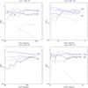 |
Fig. 1 Results of our Monte Carlo simulations on a 10 × 10 sites grain (30 Å) for environments 1, 2, 4 and 5. The solid lines represent our results for Tdust = 20 K, dashed lines for Tdust = 30 K and dotted lines Tdust = 35 K (left panel) 40 K (right panel). |
3.2. Rate equation method
The rate equation method can be applied when there is a minimum coverage of 1 atom on the dust. This condition is satisfied if the grains are not too warm, that species can encounter each other before evaporating. By comparing our rate equation results with Monte Carlo simulations, we will define a range of dust temperatures for which rate equations are valid.
The rate equation method couples the different equations for the different species on the dust. The processes described in the previous subsection are dependent on the dust and gas temperature, UV field, and exothermicity of the reaction occurring on the dust. The equation for species X can thus be written as follows: ![\begin{eqnarray} \frac{{\rm d}n(X)}{{\rm d}t} &=&n_{\rm gas}(X) v_X N_s-n(X) n(Y) \alpha_{pp}(X) \nonumber \\[3mm] & &+\, (1-f_{\rm des}) n(Y) n(Z) \alpha_{pp}(Y) -R_{{\rm evap}_X} n(X) \nonumber \\[3mm] & &-\, R_{{\rm phot}_X} n(X)+R_{{\rm phot}_Y} n(Y) \end{eqnarray}](/articles/aa/full_html/2012/01/aa17700-11/aa17700-11-eq68.png) (8)where αpp(X) and αpp(Y) are the mobilities of the species X and Y (see Eq. (5)). The different terms of this equation present (1) accretion of species X from the gas phase; (2) the formation of the new species that involve species X; (3) creation of the species X by the encountering of species Y and Z that stay on the surface; (4) evaporation of species X; (5) photodissociation of X on the dust; and (6) the creation of X by photodissociation of species Y.
(8)where αpp(X) and αpp(Y) are the mobilities of the species X and Y (see Eq. (5)). The different terms of this equation present (1) accretion of species X from the gas phase; (2) the formation of the new species that involve species X; (3) creation of the species X by the encountering of species Y and Z that stay on the surface; (4) evaporation of species X; (5) photodissociation of X on the dust; and (6) the creation of X by photodissociation of species Y.
Models parameters.
3.3. Efficiencies derived from the rate equation method
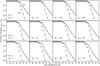 |
Fig. 2 Efficiencies for the formation of OH and H2O in low density gas (n = 103 cm-3), in atomic and molecular hydrogen dominated gas. UV fields ranging from G0 = 1 to 1000 are considered. Results from rate equations are shown by a solid and a dotted line for OH and H2O, respectively. The analytical fit is shown by the crosses (OH) and diamonds (H2O). |
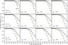 |
Fig. 3 Efficiencies for the formation of OH and H2O in high-density gas (n = 105.5 cm-3), in atomic and molecular dominated gas. UV fields ranging from G0 = 103 to 106 are considered. Results from rate equations are shown by a solid line for OH and a dotted line for H2O. The analytical fit is shown by the crosses (OH) and diamonds (H2O). |
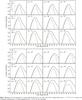 |
Fig. 4 Efficiencies for the formation of oxygen bearing species O2, O3, OH2, and H2O2 in low-density gas (n = 103 cm-3), in atomic and molecular hydrogen dominated gas. UV fields ranging from G0 = 1 to 1000 are considered. |
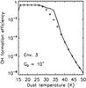 |
Fig. 5 Efficiencies for the formation of oxygen bearing species O2, O3, OH2, and H2O2 in high-density gas (n = 105.5 cm-3), in atomic and molecular dominated gas. UV fields ranging from G0 = 103 to 106 are considered. |
The formation efficiency is defined as the fraction of oxygen f(O) that is released in the gas phase in the form of another species. We studied this in a few different environments, chosen such that they resemble the conditions found in the XDR models of Meijerink & Spaans (2005). The gas temperature is fixed at a constant temperature T = 100 K, and dust temperatures ranging from Tdust = 10 − 60 K. Four different radiation fields were considered at two fixed densities, n = 103 and 105.5 cm-3, in both the atomic and molecular regimes. The parameters used are summarized in Table 2.
In Figs. 2 and 3, we show the obtained efficiencies for OH and H2O. The figures show that the efficiencies for OH and H2O are roughly constant between dust temperatures Tdust ~ 15−35 K. In this regime most of the oxygen goes to H2O. For dust temperatures Tdust ≳ 35−45 K, the total efficiency for forming molecules is rapidly decreasing, and most of the atomic oxygen will not react to another species before it evaporates from the grain. Therefore, the dust surface chemistry can only be effective when the dust temperatures are not too high. We recall that the way to form OH and H2O is through O + H → OH and OH + H → H2O. For slightly higher dust temperatures, the chance of an OH molecule evaporating from the grain becomes higher than for meeting another H atom. Therefore at temperatures Tdust ≳ 35−40 K, most of the oxygen atoms are incorporated into OH, and then ϵOH is highest.
Increasing the radiation field, has a similar effect as increasing the dust temperature, i.e., it results in a lower ϵH2O/ϵOH ratio, which is caused by photodissociation of H2O on the surface. The strongest effect is seen in environments 3 and 6, where the dominant hydrogen fraction is contained in H2. In this environment, the hydrogen accretion rates are lowest, and thus also have the lowest atomic surface density on grains. When most of the gas is in atomic form, the hydrogen accretion is such that at high dust temperatures most of the oxygen is converted into OH. However, when the gas become more and more molecular, the atomic hydrogen accretion rate onto the dust decreases, and a larger fraction of atomic oxygen ends up in O2. In environment 3, this is even the most likely product at temperature Tdust > 35 K.
In Figs. 4 and 5, the efficiencies for the formation of O2, O3, OH2, and H2O2 are shown. The efficiencies for these species show a peak at dust temperatures Tdust = 35−40 K. The maximum efficiency for producing O2 ranges from ~10-2 in the atomic gas to ~10-1 in molecular gas, and generally the efficiencies for other species are lower. At temperatures T > 40 K, O2 efficiencies dominate those for OH, but this is the regime where the formation of molecular species is not efficient.
3.4. Validity of the rate equation method
To estimate the uncertainties in the MC calculation and to check the consistency between the MC and rate equation methods, we did two additional MC simulations at dust temperatures of 20, 30, and 35 (low density) and 40 (high density). After a time t of ~1000−2000 years (low density) and ~5−10 years (high density), the efficiencies are converged and oscillate around a stable value. At Tdust = 20 and 30 K, the H2O efficiencies vary between 0.5 to 0.6, and those for OH between 0.3 to 0.4, so are very similar to the rate equation method. At the higher dust temperatures (35 and 40 K), the values obtained with the MC method are lower. The rate equation method overestimates the efficiencies, and we are entering the stochastic regime.
We only concentrate on dust temperature Tdust > 10−15 K. At very low dust temperatures, OH and H2O are still able to form at a lower efficiency, but the chemistry is different then, for a number of reasons: (1) ices can form on the surface; (2) the chemistry is different because the binding energies are different; and (3) the surface of the grain will be saturated with H2.
4. Analytical expressions for OH and H2O formation efficiencies
The rate equation method gives the populations of the different species on the dust surface, which allows us to derive a simplified analytic expression for formation efficiencies of OH and H2O that is easy to use in numerical codes. This means that the smallest set of reactions needed to reproduce the derived efficiencies from the rate equation calculation is determined. Although the analytic expression of the efficiencies is derived in Appendix A, the dependencies are given here: 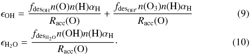 The fractions fdesOH, fdesOH′, and fdesH2O are 0.36, 0.25, and 0.15, respectively. These are the fractions of the molecules that are released in the gas phase upon formation due to the exothermicity of the reaction. The accretion rate of oxygen is Racc(O), while n(O), n(O3), and n(OH) are the dust surface densities of O, O3, and OH, respectively, in monolayers, e.g., 1 monolayer = 100% coverage. These surface densities are listed in Appendix A. The variable αH is the mobility of hydrogen atoms on the grain surface. The efficiency for the formation of water does not contain a term with accretion of OH from the gas phase, since the accretion of O followed by OH formation dominates the OH accretion.
A very important outcome of the simulation is that the formation of OH on grains is dominated by O + H → OH up to temperatures T ~ 30−40 K depending on the environment, and by O3 + H → OH + O2 at higher temperatures. This implies that, besides expressions for n(O) and n(OH), those for n(O2) and n(O3) are also needed. For completeness, we also give the one for n(H2O). The importance of the O3 + H reactions is shown in Fig. 6. It is obvious from the figure that the OH formation efficiency would be underestimated without considering the reaction with O3. These results are consistent with those obtained by Ioppolo et al. (2008), where the formation of H2O is dominated by the reaction sequence: H + O2 → HO2, H + HO2 → H2O2 followed by H + H2O2 → H2O + OH. We do consider the same reaction rate paths in our work, but in this study, molecules are formed on bare grains, while Ioppolo et al. (2008) consider icy grain mantles. In our simulation a very significant part of the molecules are desorbed upon formation, while the cycle of photodissociation of H2O and reformation on the grains significantly enhances the amount of water released in the gas phase. It does not require the complex route through H2O2. There is also another way to form H2O that involves O3. The reaction O + O2 → O3 releases only a very small part into the gas phase upon formation (only a few percent), so although the efficiency for the formation of O3 is low, there is a significant amount of O3 on the surface to react to OH. The work by Hollenbach et al. (2009) is also very different from ours. They also treat a surface chemistry network, with H2, OH, O2, and some other different species, such as CH, CH2, and CH3. They do not include processes with O3 and H2O2, intermediate species in the processes leading to water formation. However, the biggest difference between our models are the dominant processeses for delivering species back into the gas phase which are thermal, photo, and cosmic-ray desorption in the Hollenbach et al. (2009) paper, since they consider ices in that work. In our work, this is desorption upon formation. They consider a PDR environment, and therefore they allow for the formation of strongly bound icelayers. We assume that this does not occur because of the turbulent motions stripping the grains and the strong photodissociating radiation fields that are internally created by X-rays.
The approximate analytical fits to the rate equation results are very good for environments 1, 2, 4, and 5. However, environment 3 and 6, which are highly molecular, start to show deviations for dust temperatures Tdust > 30 K for the H2O. This is due to additional reactions on the grain surface, that we did include in the rate equation method, but not in the approximate fit.
The fits should not be applied at very low dust temperatures (Tdust) < 10 K, because the analytical fits do not match the MC and rate equation results.
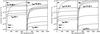 |
Fig. 6 Efficiencies for environment 3, largely molecular, low density n = 103 cm-3 gas, G0 = 104: result from rate equation simulation (solid line), with (dotted line) and without (crosses) including of the reaction O3 + H → OH + O2 in the analytical expression. |
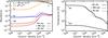 |
Fig. 7 Comparison of dust and gas phase reaction rates at n = 105,5 cm-3 for an environment with low (left, xH = 1, xH2 = 3 × 10⁻⁴) and high molecular abundances (right, xH = 10-2, xH2 = 0.5) as a function of gas temperature for dust temperatures Tdust = 15, 30, 45, 60, 75, and 90 K. The OH abundances are varied between xOH = 10-8, 10-7, and 10-6 at low and 10-6, 10-5, and 10-4 at high molecular abundances. This resembles the unshielded and shielded environment of model 4 in Meijerink & Spaans (2005). |
 |
Fig. 8 X-ray irradiated cloud with density n = 105.5 cm-3 and radiation field FX = 160 erg cm-2 s-1. (left) The abundances are shown for H, H2, OH, and H2O in three different cases: formation of OH and H2O (i) in gas phase only (ii) in gas phase and on dust with an MRN size distribution, and (iii) in gas phase and on dust with a Weingartner & Draine size distribution. (right) Gas and dust temperatures for the same models. The temperature profiles for the gas only models and those where OH and H2O formation on dust with an MRN distribution are included are the same. |
5. OH and H2O formation: gas versus dust
To estimate the importance of OH and H2O formation on dust grains, a comparison is made to the gas phase neutral-neutral formation rates, which are given by (UMIST database: Le Teuff et al. 2000; Woodall et al. 2007) 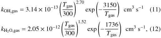 while the conservative dust phase reaction rates (using the cross sections from the MRN distribution, ndustσ/n(H) = 10-21 cm-2), are given by
 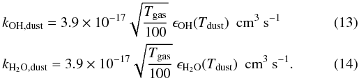 Depending on the environment (i.e., the ambient atomic and molecular abundances, gas and dust temperature, etc.), OH and H2O form premarily on the dust grains or in the gas phase:
-
Although the efficiency for formation of OH and H2O on dust strongly depends on the dust temperature Tdust, the variations with gas temperature Tgas at a fixed dust temperature Tdust are very modest.
-
The gas phase formation rates have high activation barriers of Tgas = 3150 and 1736 K for the formation of OH and H2O, respectively. These channels are essentially cut off below temperatures Tgas ≲ 200 K.
-
Formation on dust depends on abundances of O and H, and in the gas phase on H2, O, and OH.
For illustration purposes, a comparison between the gas and dust phase formation rates are shown for two different regimes in Fig. 7, a mostly atomic (left) and molecular (right) environment. We do not show the ion-molecule reaction rates, even though they are considered in our chemical network. These processes can be more efficient than the neutral reaction chain at low gas temperatures, which is a domain that we do not consider in this study. The abundunces resemble the unshielded and shielded regions of model 4 in Meijerink & Spaans (2005) with density n = 105.5 cm-3: the atomic environment has abundances xH = 1, xH2 = 3 × 10⁻⁴, xO = 3 × 10⁻⁴, xOH = 10-8, 10-7, and 10-6 (left), and the molecular environment has abundances xH = 10-2, xH2 = 0.5, xO = 2 × 10⁻⁴, and xOH = 10-6, 10-5, and 10-4 (right). We adopt a range of OH abundances, to show the effect on the gas phase rates. We should note here that the OSU astrochemistry database1 (maintained by Eric Herbst) claims a lower rate at high temperatures T > 500 for the H2 + OH reaction, and is given by kH2O,gas = 8.4 × 10⁻¹³ exp(−1040/Tgas). This would make the dust surface reaction even more important.
The efficiencies ϵOH and ϵH2O are reasonably high, ~0.3 and ~0.6, respectively, at dust temperatures Tdust < 40 K. As a result, the H2O dust formation rate is always dominating the gas phase formation in the atomic environment, while the OH dust formation is more important at temperatures Tgas < 800 K. Even though OH and H2O formation efficiencies drop very fast for higher dust temperatures, molecule formation with dust as catalyst will always become dominant below a certain gas temperature. The break-even point ranges from Tgas ~ 100−400 K depending on the dust temperature Tdust = 45 − 90 K. We should keep in mind though that for Tdust > 35−40 K, the formation rates are overestimated in our model.
This picture is different in a molecular environment. Even when the OH and H2O formation efficiencies are high (Tdust < 40 K), gas phase formation is more efficient at gas temperatures Tgas > 100 − 200 K. Where in the atomic environment, the OH and H2O gas phase formation is suppressed by the very low abundances of H2, the dust phase formation rate is suppressed due to the low accretion rate of atomic hydrogen, which is depleted by two orders of magnitude. In the molecular environment, the formation of water in either the dust or gas phase is inefficient through neutral-neutral reactions, and ion-molecule reactions will also contribute significantly or even dominate, through the chain O + + H2 → OH + + H, OH + + H2 → H2O + + H, H2O + + H2 → H3O + + H, followed by recombination H3O + + e − → H2O + H.
6. Application to X-ray environments
The inner regions of active galaxies from, e.g., Mrk 231, which are highly exposed to X-rays, are likely to exhibit enhanced formation of H2O on dust grains: (i) dust temperatures are expected to be moderate, Tdust ~ 20 − 40 K, as the heating of dust is less efficient than by UV; (ii) the dynamical timescales are not very long and shocks are expected to be present, so dust particles are not expected to be or stay covered with ice; (iii) shocks may even be able to break up grains into smaller particles, therefore enlarging the effective surface of dust, where water is expected to form.
In Fig. 8, the chemical abundances of H, H2, OH and H2O and temperatures of an XDR model are shown with density n = 105.5 cm-3, FX = 160 erg cm-2 s-1, and solar metallicity, Z = Z⊙. Three different cases for the formation of OH and H2O are considered:
-
1.
Gas phase only: The OH abundance isxOH ~ 3 × 10⁻⁷ at low column densities, rising to ~ 10-5 just before the H/H2 transition, leveling off to 10-6. The H2O abundance is xH2O ~ 10-10 at column densities
 cm-2. As OH, H2O becomes more and more abundant toward the H/H2 transition, and reaches an abundance xH2O ~ 10-6 beyond NH ~ 1023 cm-2.
 -
2.
Gas and dust with an MRN distribution: nothing changes for OH. As shown in Fig. 7, the OH gas phase formation is more important at gas temperatures T > 800 K, at all dust temperatures. The abundance of H2O, however, is higher by a factor 8, at low column densities NH < 1022 cm-2, and thus the integrated column of warm water (T ≳ 200 K). At low temperatures (i.e., at high column densities, NH ≳ 1023 cm-2), nothing changes for OH and H2O, because the formation route is dominated by the ion-molecule reactions.
-
3.
Gas and dust with a Weingartner & Draine distribution: the H2 formation rate is now higher as well due to the higher surface area of the dust grains. As a result a small increase is seen in the H2 abundance at low column densities. At the same time, the H/H2 transition occurs at lower column densities, NH ~ 2 × 1023 cm-2, compared to NH ~ 3 × 1023 cm-2 compared to the gas phase model. As a result, the OH also peaks at a lower column density, and reaches a slightly higher peak abundance. The OH enhancement is due to a higher gas phase formation rate, as a result of the higher H2 abundance, not because of the higher formation rate on dust. The water abundance in the high temperature range is enhanced by more than an order of magnitude. As the H/H2 transition occurs at lower column densities, the rise in the water abundance also occurs at these lower column densities.
To summarize, we find that the warm H2O colunmn density is enhanced by approximately an order of magnitude over a column NH ~ 5 × 1022 cm-2, when including H2O formation on dust. At higher column densities, where temperatures decrease and the gas becomes molecular, the formation on dust grains does not affect the abundance of H2O. The OH abundance is only indirectly affected by the higher H2 formation rate on dust when using the Weingartner & Draine (2001) distribution with the higher dust cross section.
7. Discussion and conclusions
The role and importance of OH and H2O formation on dust was investigated. We used both Monte Carlo and rate equation simulations to determine the efficiency at which oxygen is converted into OH and H2O on dust grains. The rate equation method is very fast, and is used to calculate a grid of different environments, both low and high density ones (n = 103 and 105.5 cm-3), and different molecular fractions, radiation fields, and temperatures (see Figs. 2 and 3). The Monte Carlo simulations are used as a consistency check, and because these simulations are fairly slow, efficiencies are only calculated for a limited number of dust temperatures. At dust temperatures Tdust < 35−40 K, the Monte Carlo and rate equation method yield the same results, within the uncertainties. At higher dust temperatures, the efficiencies obtained by the two methods start to deviate: the rate equation method systematically obtains higher efficiences than the MC method. This is where the process of OH and H2O formation on dust enters the stochastic regime. We fitted analytical expression to the derived results from the rate equations, such that they are easy to implement in any chemistry code. We find the follwing:
-
OH formation on grains and release to gas phase is dominated byO + H → OH (Tdust < 35 − 40 K and by O3 + H → OH + O2 (for higher dust temperatures). The high dust temperatures result in decreasing hydrogen surface densities, because of the increasing evaporation rates.
-
H2O formation on grains and release to gas phase is dominated by OH + H → H2O.
-
The fraction of OH that is released in the gas upon formation is on the order of 36% and for H2O it is 9%. However, in strong UV radiation fields, water on the dust can be photodissociated, and then reform to water, which then gives another contribution to the gas phase. This loop of forming-dissociating-forming increases the effective fraction of H2O released in the gas by a factor 5.
-
A comparison of gas and dust phase formation rates (see Fig. 7) shows that formation on dust grains is important for dust temperatures lower than 40 K.
We implemented the analytical expressions for the formation rates in the Meijerink & Spaans (2005) XDR code, and calculated a model with parameters representative of the inner regions of active galaxies. We find that the additional processes enhances the integrated column density of warm water. This increased column helps explain unusually strong water lines observed for Mrk 231, which has an accreting supermassive black hole with X-ray luminosity LX ~ 1044 erg s-1. This ULIRG shows, for example, a very high H2O 202 − 111/CO J = 8 − 7 ratio. These ratios are not observed in typical starforming environments that are mainly exposed to UV-only (PDR) environments, such as the one observed in the Orion Bar (Habart et al. 2010) or M 82 (Panuzzo et al. 2010), where this ratio is typically an order of magnitude or more less than in Mrk 231, and as such these very bright H2O lines might be typical of regions that are exposed to high X-ray fluxes, close to the accreting black hole in active galaxies.
Acknowledgments
We thank the anonymous referee for a careful reading of the manuscript and a constructive report that significantly improved the paper.
References
- Akai, Y., & Saito, S. 2003, Jpn. J. Appl. Phys., 42, 640 [NASA ADS] [CrossRef] [Google Scholar]
- Andersson, S., & van Dishoeck, E. F. 2008, A&A, 491, 907 [NASA ADS] [CrossRef] [EDP Sciences] [Google Scholar]
- Andersson, S., Al-Halabi, A., Kroes, G.-J., & van Dishoeck, E. F. 2006, J. Chem. Phys., 124, 064715 [NASA ADS] [CrossRef] [Google Scholar]
- Bergeron, H., Rougeau, N., Sidis, V., Teillet-Billy, D., & Aguillon, F. 2008, J. Phys. Chem. A, 112, 11921 [CrossRef] [PubMed] [Google Scholar]
- Boksenberg, A., Carswell, R. F., Allen, D. A., et al. 1977, MNRAS, 178, 451 [NASA ADS] [Google Scholar]
- Braito, V., Della Ceca, R., Piconcelli, E., et al. 2004, A&A, 420, 79 [NASA ADS] [CrossRef] [EDP Sciences] [Google Scholar]
- Cazaux, S., & Tielens, A. G. G. M. 2002, ApJ, 575, L29 [NASA ADS] [CrossRef] [Google Scholar]
- Cazaux, S., & Tielens, A. G. G. M. 2004, ApJ, 604, 222 [NASA ADS] [CrossRef] [Google Scholar]
- Cazaux, S., Cobut, V., Marseille, M., Spaans, M., & Caselli, P. 2010, A&A, 522, A74 [NASA ADS] [CrossRef] [EDP Sciences] [Google Scholar]
- Cuppen, H. M., & Herbst, E. 2007, ApJ, 668, 294 [Google Scholar]
- Cuppen, H. M., Ioppolo, S., Romanzin, C., & Linnartz, H. 2010a, Phys. Chem. Chem. Phys., 12, 12077 [NASA ADS] [CrossRef] [Google Scholar]
- Cuppen, H. M., Kristensen, L. E., & Gavardi, E. 2010b, MNRAS, 406, L11 [NASA ADS] [Google Scholar]
- Draine, B. T. 1995, Ap&SS, 233, 111 [NASA ADS] [CrossRef] [Google Scholar]
- Fischer, J., Sturm, E., González-Alfonso, E., et al. 2010, A&A, 518, L41 [NASA ADS] [CrossRef] [EDP Sciences] [Google Scholar]
- Galli, D., & Palla, F. 1998, A&A, 335, 403 [NASA ADS] [Google Scholar]
- Glover, S. C. O. 2003, ApJ, 584, 331 [NASA ADS] [CrossRef] [Google Scholar]
- González-Alfonso, E., Fischer, J., Isaak, K., et al. 2010, A&A, 518, L43 [NASA ADS] [CrossRef] [EDP Sciences] [Google Scholar]
- Habart, E., Dartois, E., Abergel, A., et al. 2010, A&A, 518, L116 [NASA ADS] [CrossRef] [EDP Sciences] [Google Scholar]
- Hollenbach, D. J., & Tielens, A. G. G. M. 1999, Rev. Mod. Phys., 71, 173 [Google Scholar]
- Hollenbach, D., Kaufman, M. J., Bergin, E. A., & Melnick, G. J. 2009, ApJ, 690, 1497 [CrossRef] [Google Scholar]
- Hornekær, L., Rauls, E., Xu, W., et al. 2006, Phys. Rev. Lett., 97, 186102 [NASA ADS] [CrossRef] [PubMed] [Google Scholar]
- Ioppolo, S., Cuppen, H. M., Romanzin, C., van Dishoeck, E. F., & Linnartz, H. 2008, ApJ, 686, 1474 [NASA ADS] [CrossRef] [Google Scholar]
- Ioppolo, S., Cuppen, H. M., Romanzin, C., van Dishoeck, E. F., & Linnartz, H. 2010, Phys. Chem. Chem. Phys., 12, 12065 [NASA ADS] [CrossRef] [Google Scholar]
- Jelea, A., Marinelli, F., Ferro, Y., Allouche, A., & Brosset, C. 2008, J. Phys. Chem. A, 112, 11921 [CrossRef] [PubMed] [Google Scholar]
- Katz, N., Furman, I., Biham, O., Pirronello, V., & Vidali, G. 1999, ApJ, 522, 305 [NASA ADS] [CrossRef] [Google Scholar]
- Launay, J. M., Le Dourneuf, M., & Zeippen, C. J. 1991, A&A, 252, 842 [NASA ADS] [Google Scholar]
- Le Teuff, Y. H., Millar, T. J., & Markwick, A. J. 2000, A&AS, 146, 157 [NASA ADS] [CrossRef] [EDP Sciences] [MathSciNet] [PubMed] [Google Scholar]
- Lee, G., Lee, B., Kim, J., & Cho, K. 2009, J. Phys. Chem. C, 113, 14225 [CrossRef] [Google Scholar]
- Maloney, P. R., Hollenbach, D. J., & Tielens, A. G. G. M. 1996, ApJ, 466, 561 [NASA ADS] [CrossRef] [Google Scholar]
- Mathis, J. S., Rumpl, W., & Nordsieck, K. H. 1977, ApJ, 217, 425 [NASA ADS] [CrossRef] [Google Scholar]
- Meijerink, R., & Spaans, M. 2005, A&A, 436, 397 [NASA ADS] [CrossRef] [EDP Sciences] [Google Scholar]
- Miyauchi, N., Hidaka, H., Chigai, T., et al. 2008, Chem. Phys. Lett., 456, 27 [NASA ADS] [CrossRef] [Google Scholar]
- Mokrane, H., Chaabouni, H., Accolla, M., et al. 2009, ApJ, 705, L195 [NASA ADS] [CrossRef] [Google Scholar]
- Morisset, S., Aguillon, F., Sizun, M., & Sidis, V. 2004, J. Chem. Phys., 121, 6493 [NASA ADS] [CrossRef] [Google Scholar]
- Neufeld, D. A., & Kaufman, M. J. 1993, ApJ, 418, 263 [NASA ADS] [CrossRef] [Google Scholar]
- Neufeld, D. A., Lepp, S., & Melnick, G. J. 1995, ApJS, 100, 132 [NASA ADS] [CrossRef] [Google Scholar]
- Nisini, B., Benedettini, M., Giannini, T., et al. 1999, A&A, 350, 529 [NASA ADS] [Google Scholar]
- Panuzzo, P., Rangwala, N., Rykala, A., et al. 2010, A&A, 518, L37 [NASA ADS] [CrossRef] [EDP Sciences] [Google Scholar]
- Papadopoulos, P. P., van der Werf, P., Isaak, K., & Xilouris, E. M. 2010, ApJ, 715, 775 [NASA ADS] [CrossRef] [Google Scholar]
- Pirronello, V., Liu, C., Roser, J. E., & Vidali, G. 1999, A&A, 344, 681 [NASA ADS] [Google Scholar]
- Sha, X. 2002, Surface Science, 496, 318 [NASA ADS] [CrossRef] [Google Scholar]
- Sha, X., Jackson, B., Lemoine, D., & Lepetit, B. 2005, J. Chem. Phys., 122, 014709 [NASA ADS] [CrossRef] [MathSciNet] [Google Scholar]
- Sturm, B., Bouwman, J., Henning, T., et al. 2010, A&A, 518, L129 [NASA ADS] [CrossRef] [EDP Sciences] [Google Scholar]
- van der Werf, P. P., Isaak, K. G., Meijerink, R., et al. 2010, A&A, 518, L42 [NASA ADS] [CrossRef] [EDP Sciences] [Google Scholar]
- van Kempen, T. A., Green, J. D., Evans, N. J., et al. 2010, A&A, 518, L128 [NASA ADS] [CrossRef] [EDP Sciences] [Google Scholar]
- Wagner, A. F., & Graff, M. M. 1987, ApJ, 317, 423 [NASA ADS] [CrossRef] [Google Scholar]
- Weingartner, J. C., & Draine, B. T. 2001, ApJ, 548, 296 [NASA ADS] [CrossRef] [Google Scholar]
- Woodall, J., Agúndez, M., Markwick-Kemper, A. J., & Millar, T. J. 2007, A&A, 466, 1197 [NASA ADS] [CrossRef] [EDP Sciences] [Google Scholar]
- Zecho, T., Guttler, A., Sha, X., Jackson, B., & Kuppers, J. 2002, J. Chem. Phys., 117, 8486 [NASA ADS] [CrossRef] [Google Scholar]
Appendix A: OH and H2O formation efficiencies
The formation efficiency with which gas-phase OH and H2O are formed can be written as a balance between the desorption fraction from the grain upon formation and the accretion rate of oxygen atoms onto the grain. On grains, two formation processes play a major role for OH in different dust temperature regimes, while for H2O, there is only one major formation route: 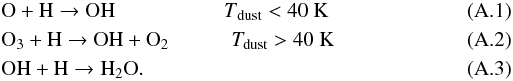 Therefore, the efficiencies should be written as
 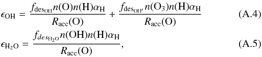 where n(H), n(O), n(O3), and n(OH) are the surface density of H, O, O3, and OH on the dust. These hydrogen and oxygen atoms are accreted from the gas phase at a rate of
 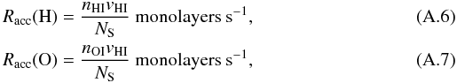 where nHI and nOI are the densities of atomic hydrogen and oxygen in the gas phase, vHI and vOI the mean velocities of these atoms:
  and
and  × 1014 cm-2 the number of sites per cm2. The H atoms arrive on the dust surface in physisorbed sites, and then continue to a chemisorbed site or evaporate from the surface. As a result, the density on the surface can be written as
  (A.10)The mobility for hydrogen atoms to enter into a chemisorbed site is mostly due to tunneling, which we can then approximate by
  × 10-3, where apc and EA are the width and the height of the barrier between physisorbed and chemisorbed sites. The adopted values are apc = 1.5 Å and EA = 2870 K. The hydrogen surface density can then be calculated as
 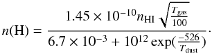 (A.11)The formation of OH and H2O can be determined analytically from the rate equations, when the most important processes are considered. The rate equations of O, OH, and H2O, as well as O2 and O3, are considered here, since the efficiency of OH depends on the abundance of O3 as well. The abundance change as a function of time for these species are given by the following expressions:
 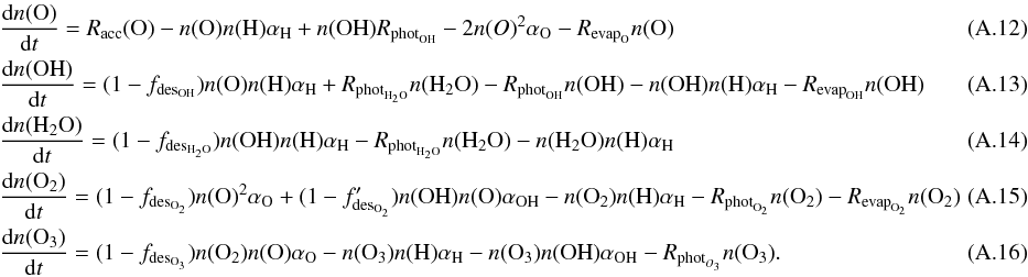 When we consider the surface densities of the species at steady state, the surface densities of the species become
 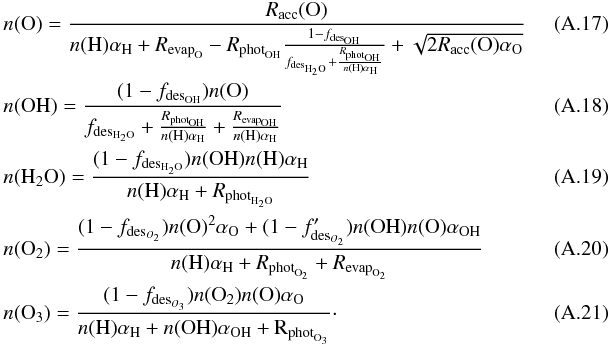 Filling in the equations for the various included reactions, the expressions become as follows:
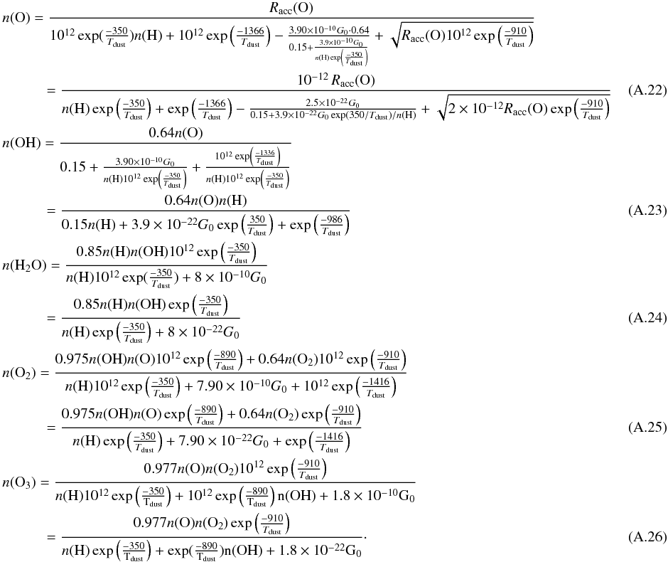
Adopted photodissociation rates in the approximation.
All Tables
All Figures
|
Fig. 1 Results of our Monte Carlo simulations on a 10 × 10 sites grain (30 Å) for environments 1, 2, 4 and 5. The solid lines represent our results for Tdust = 20 K, dashed lines for Tdust = 30 K and dotted lines Tdust = 35 K (left panel) 40 K (right panel). |
| In the text | |
|
Fig. 2 Efficiencies for the formation of OH and H2O in low density gas (n = 103 cm-3), in atomic and molecular hydrogen dominated gas. UV fields ranging from G0 = 1 to 1000 are considered. Results from rate equations are shown by a solid and a dotted line for OH and H2O, respectively. The analytical fit is shown by the crosses (OH) and diamonds (H2O). |
| In the text | |
|
Fig. 3 Efficiencies for the formation of OH and H2O in high-density gas (n = 105.5 cm-3), in atomic and molecular dominated gas. UV fields ranging from G0 = 103 to 106 are considered. Results from rate equations are shown by a solid line for OH and a dotted line for H2O. The analytical fit is shown by the crosses (OH) and diamonds (H2O). |
| In the text | |
|
Fig. 4 Efficiencies for the formation of oxygen bearing species O2, O3, OH2, and H2O2 in low-density gas (n = 103 cm-3), in atomic and molecular hydrogen dominated gas. UV fields ranging from G0 = 1 to 1000 are considered. |
| In the text | |
|
Fig. 5 Efficiencies for the formation of oxygen bearing species O2, O3, OH2, and H2O2 in high-density gas (n = 105.5 cm-3), in atomic and molecular dominated gas. UV fields ranging from G0 = 103 to 106 are considered. |
| In the text | |
|
Fig. 6 Efficiencies for environment 3, largely molecular, low density n = 103 cm-3 gas, G0 = 104: result from rate equation simulation (solid line), with (dotted line) and without (crosses) including of the reaction O3 + H → OH + O2 in the analytical expression. |
| In the text | |
|
Fig. 7 Comparison of dust and gas phase reaction rates at n = 105,5 cm-3 for an environment with low (left, xH = 1, xH2 = 3 × 10⁻⁴) and high molecular abundances (right, xH = 10-2, xH2 = 0.5) as a function of gas temperature for dust temperatures Tdust = 15, 30, 45, 60, 75, and 90 K. The OH abundances are varied between xOH = 10-8, 10-7, and 10-6 at low and 10-6, 10-5, and 10-4 at high molecular abundances. This resembles the unshielded and shielded environment of model 4 in Meijerink & Spaans (2005). |
| In the text | |
|
Fig. 8 X-ray irradiated cloud with density n = 105.5 cm-3 and radiation field FX = 160 erg cm-2 s-1. (left) The abundances are shown for H, H2, OH, and H2O in three different cases: formation of OH and H2O (i) in gas phase only (ii) in gas phase and on dust with an MRN size distribution, and (iii) in gas phase and on dust with a Weingartner & Draine size distribution. (right) Gas and dust temperatures for the same models. The temperature profiles for the gas only models and those where OH and H2O formation on dust with an MRN distribution are included are the same. |
| In the text | |
Current usage metrics show cumulative count of Article Views (full-text article views including HTML views, PDF and ePub downloads, according to the available data) and Abstracts Views on Vision4Press platform.
Data correspond to usage on the plateform after 2015. The current usage metrics is available 48-96 hours after online publication and is updated daily on week days.
Initial download of the metrics may take a while.