| Issue |
A&A
Volume 534, October 2011
|
|
|---|---|---|
| Article Number | A29 | |
| Number of page(s) | 14 | |
| Section | Galactic structure, stellar clusters and populations | |
| DOI | https://doi.org/10.1051/0004-6361/201117630 | |
| Published online | 26 September 2011 | |
Chemical enrichment mechanisms in ω Centauri: clues from neutron-capture elements ⋆
1
INAF − Osservatorio Astronomico di Padova, vicolo dell’Osservatorio 5, 35122 Padova, Italy
e-mail: This email address is being protected from spambots. You need JavaScript enabled to view it.
; This email address is being protected from spambots. You need JavaScript enabled to view it.
; This email address is being protected from spambots. You need JavaScript enabled to view it.
2
INAF − Osservatorio Astronomico di Bologna, via Ranzani 1, 40127 Bologna, Italy
e-mail: This email address is being protected from spambots. You need JavaScript enabled to view it.
; This email address is being protected from spambots. You need JavaScript enabled to view it.
; This email address is being protected from spambots. You need JavaScript enabled to view it.
;
3
Department of Astronomy and McDonald Observatory, The University of Texas, Austin TX 78712, USA
e-mail: This email address is being protected from spambots. You need JavaScript enabled to view it.
Received: 5 July 2011
Accepted: 18 August 2011
Abstract
Context. In the complex picture of multiple stellar populations in globular clusters (GCs), a special role is played by NGC 5139 (ω Centauri). At variance with the majority of GCs, ω Cen exhibits significant star-to-star variations in metallicity and in relative neutron-capture element abundance ratios with respect to Fe, along with split evolutionary sequences as revealed from colour–magnitude diagrams. Combining information from photometry and spectroscopy, several studies suggested that an age spread of several Gyr has to be invoked to explain (at least partially) some of the observed features. However, a comprehensive understanding of the formation, evolution and chemical enrichment processes is still not at hand.
Aims. Relatively metal-rich ω Cen stars display neutron-capture abundance distributions dominated by contributions from the s-process, but it is not clear what roles have been played by the so-called main and weaks-process components in generating these abundances. To gain better insight into this question we derived lead (Pb) abundances for several ω Cen cluster members, because this element can only be produced by the mains-process.
Methods. We analysed high-resolution UVES@VLT spectra of a sample of twelve red-giant branch stars, deriving abundances of Pb and also of Y, Zr, La, Ce, Eu, and the C+N+O sum. Spectral synthesis was applied to all features, taking into account isotopic shifts and/or hyperfine structure as needed.
Results. We measured for the first time the Pb content in ω Cen, discovering a clear hint for a Pb production occurring at [Fe/H] > −1.7 dex. Our data suggest that the role of the weak component in the production of s-process elements is negligible. Moreover, evidence gathered from the abundances of other elements indicates that the main component occurring in this GC is peculiar and shifted towards higher mass polluters than the standard one.
Key words: stars: abundances / stars: Population II / globular clusters: individual:ωCentauri (NGC 5139)
Based on data obtained with the ESO UVES spectrograph during the observing programmes 165.L-0263 and 67.D-0245.
© ESO, 2011
1. Introduction
About 30 years ago new efficient medium-high resolution spectrometers began appearing on very large telescopes, allowing the acquisition of high-quality, high S/N spectra for large samples of globular cluster (GC) stars. This new technology led to extensive spectroscopic surveys that substantially modified the classical view of cluster birth and evolution. For a couple of decades now we have understood that many (all?) GCs exhibit significant star-to-star variations in their light-element contents (see Kraft 1994; Gratton et al. 2004; Martell 2011, for reviews of these discoveries).
Photometric colour-magnitude observations have revealed split evolutionary sequences in a handful of GCs (e.g. Lee et al. 1999; Pancino et al. 2000; Bedin et al. 2004; Milone et al. 2008; Han et al. 2009). But it has taken high-resolution spectroscopy to truly establish the complex nature of GCs. With their peculiar abundance pattern, GCs are fundamentally different from the other Galactic stellar populations (young/old open clusters, see e.g., Gratton et al. 2004; de Silva et al. 2009; Pancino et al. 2010a; Bragaglia et al. 2011).
Analysing a sample of more than 1500 giants in 19 GCs, Carretta et al. (2009a,b) concluded that all the surveyed GCs, although characterised by a homogeneous composition in iron-peak and the heavy α-elements (e.g., Ca and Ti), present variations in light elements. These variations do not occur randomly: the abundances of CH − CN, O − Na, and Mg − Al are anticorrelated with each other in stars at all evolutionary stages (e.g., Cohen 1999; Kayser et al. 2008; Pancino et al. 2010b; Carretta et al. 2009a,b; Lind et al. 2009). Globular clusters contain stars with high O (Mg, and C) and low Na (Al, and N) abundances, which constitute the primordial cluster population (first-generation stars), and stars with considerable enhancement in Na, Al, and N accompanied by depletion in O (Mg, and C), which are second-generation stars. The light-element abundance pattern of the second-generation stars (which can be seen in stars of all evolutionary stages) can be identified with hot H-burning nucleosynthesis (Denisenkov & Denisenkova 1989; Langer et al. 1993). However, the nature of element-donating stars of the previous generation, whose ashes provided the material from which second-generation stars formed, is still uncertain. Various scenarios, none universally-accepted yet, have been proposed: intermediate-mass AGB stars (Ventura et al. 2001); fast rotating massive stars (Decressin et al. 2007); and massive binaries (de Mink et al. 2009).
The abundances of neutron-capture elements (n-capture, Z > 30) generally show little star-to-star scatter in most GCs (Armosky et al. 1994; James et al. 2004). Typically an n-capture distribution more heavily weighted towards the r-process1 than the s-process is apparent in GCs, most easily seen in ratios [Eu/Ba] ≈ + 0.4 (as summarized by Gratton et al. 2004). Recently, D’Orazi et al. (2010) have shown that the s-process-dominated element barium (Ba) is mostly characterized by a single abundance value within individual GCs (see however Roederer 2011, for the spread in r-process elements within some GCs).
In addition to the “prototypical” GCs, like NGC 6752 (see Carretta et al. 2009b; Pasquini et al. 2005; Shen et al. 2011), the large family of GCs includes some peculiar cases. The very metal-poor GC M15 (NGC 7078) has large star-to-star r-process scatter (e.g. δ[Eu/Fe] ≈ 0.5; Sneden et al. 1997; Sobeck et al. 2011). In contrast, M22 (NGC 6656) exhibits an overall metallicity variation (δ[Fe/H] ~ 0.15) that is positively correlated with the variations in s-process elements (e.g. δ[Ba, Y, Zr/Fe] ≈ 0.4; Marino et al. 2009). In NGC 1851, Yong & Grundahl (2008) found a scatter in [Fe/H] of 0.09 dex, while a slightly smaller variation (i.e., δ[Fe/H] ≈ 0.06) has been detected by Carretta et al. (2010a). Ba seems instead to vary from a factor of four to more than one dex (Yong & Grundahl 2008; Villanova et al. 2010; and Carretta et al. 2011). Looking outside our Galaxy, M 54 (NGC 6715), currently located in the centre of the Sagittarius dwarf spheroidal galaxy (e.g., Bellazzini et al. 2008), has been recently scrutinised by Carretta et al. (2010b). This work confirmed the presence of an internal iron spread, as previously suggested by e.g., Sarajedini & Layden (1995), of about 0.19 dex (rms), with the bulk of stars at [Fe/H] ~ −1.6 and a long tail extended at higher metallicity. Finally, in the bulge metal-poor GC NGC 6522 Barbuy et al. (2009) found a spread in the Ba content of about ~0.5 dex (rms) by analysing eight stars (see Chiappini et al. 2011, for a more detailed discussion).
However, the most intriguing and spectacular case of a complex GC is ω Centauri (NGC 5139). It is the most massive GC of our Galaxy, with a total mass of 2.5 × 10⁶ M⊙ (van de Ven et al. 2006). It has been the object of many photometric investigations since the 1960s (e.g. Wooley 1966; Anderson 1998; Pancino et al. 2000; Bedin et al. 2004; Ferraro et al. 2004; Sollima et al. 2005a,b, 2007; Bellini et al. 2010). All these works found the presence of split evolutionary sequences, from the main-sequence (MS), to the subgiant branch (SGB) all the way to the red-giant branch (RGB) tip. At the same time, spectroscopic surveys revealed variations in [Fe/H] up to a factor of ~10 and a steep trend with Fe of n-capture elements La and Ba (e.g., Norris & Da Costa 1995; Smith et al. 2000, hereafter S00).
Recently Johnson & Pilachowski (2010, JP10) published an extensive spectroscopic study for a sample of more than 850 RGB stars in ω Cen, building up the most comprehensive database of this kind available so far. The authors confirmed that the metallicity ranges from [Fe/H] ≈ − 2 to [Fe/H] ≈ − 0.5, and that abundances for heavy α-elements (e.g. Si, Ca, Ti) and Fe-peak ones (e.g. Sc, Ni) satisfactorily match a type-II SN abundance pattern. On the other hand, the light elements (O, Na, Al) present variations larger than 0.5 dex and exhibit the classical GC proton-capture anticorrelation trends at almost all metallicities (with the exception of the most metal-rich stars). JP10 found a roughly constant [α/Fe] ratio, which they argue rules out a significant contribution from type-Ia SN (see however Pancino et al. 2002; Origlia et al. 2003, for a different view). Finally among the n-capture elements, [La/Fe] strongly increases with [Fe/H], not matched by a similar trend in [Eu/Fe] (JP10), suggesting that at [Fe/H] ≳ − 1.6, the s-process becomes the dominant n-capture production mechanism. This clearly implies that long-duration timescales ( ≳ 1 Gyr) are required for the evolution of low-mass AGB, where the main component of the s-process production occurs.
Similar conclusions were also drawn by Marino et al. (2011, M11), who analysed more than 300 ω Cen giants. In trying to solve the problems of timescales in the evolution of various abundance signatures, M11 speculated that the so-called weak s-process component (see e.g. Raiteri et al. 1993; Travaglio et al. 2004) might perhaps be responsible for the enhancement in s-process elements. The weak component, whose source are probably massive AGB stars, is responsible for substantial amounts of the solar-system s-process isotopes up to A = 90 but contributes vanishingly small amounts of heavier material. The so-called main component accounts for the heaviest s-process element abundances (i.e. beyond Zr), and its production site has been ascribed to thermally pulsing low-mass AGBs (M/M⊙ ~ 1–3). Marino et al. suggested that at the lower metallicities characteristic of ω Cen, the weak component might produce heavier n-capture elements, up to Ba and La, owing to the higher neutron over iron-seed ratio.
To test this prediction, and in general to observationally constrain element enrichment timescales, we have conducted a new high-resolution spectroscopy study of 12 ω Cen RGB stars in the rarely-studied blue spectral region. For this stellar sample we have derived abundances for Y, Zr, La, Ce, and Eu, and estimated the C+N+O abundance sums. More importantly, we have derived for the first time lead (Pb) abundances in ω Cen. In the s-process, Pb can only be produced by the main component. Detection of significant amounts of Pb in ω Cen giants indicates that the main component has played a significant role in the production of the s-process elements in this GC.
The paper is organised as follows: in Sect. 2 we give information on the sample stars, data reduction and abundance analysis. Our results are illustrated in Sect. 3, while their scientific implications are discussed in Sect. 4. A summary is given in Sect. 5.
2. Observations and analysis
2.1. Sample stars and data reduction
We considered a sample of 12 ω Cen RGB stars, covering the whole metallicity range, i.e. from [Fe/H] ≈ −2 to [Fe/H] ≈ −0.5. In Table 1 we present their basic data. For each star, Col. 1 has the “Leiden” stellar designation (van Leeuwen et al. 2000); Col. 2 has the older “ROA” number (Woolley 1966); Cols. 3–5 have broad-band photometry; and columns 6−9 have model atmosphere parameters Teff, log g, [Fe/H], and ξ that we have adopted from JP10. While our sample is small and biased towards high metallicity with respect to the bulk of ω Cen stars, these targets cover an interesting range for studying the enrichment of n-capture elements.
Identification, photometry, and adopted parameters for our programme stars (see JP10).
One of the stars presented in this paper, ROA 211 (Woolley 1966), or Leiden #60073 (van Leeuwen et al. 2000), has already been studied by Pancino et al. (2002). Its spectrum was obtained in June 2000 with the UVES spectrograph mounted at the ESO VLT, Paranal observatory, Chile. We used the 1″-wide slit; the spectral resolving power was R ≡ λ/δλ ≈ 45 000. Signal-to-noise ratios – per pixel – near 6000 Å are higher than 100, while around the Pb i lines at 3683 Å and 4058 Å we have S/N ~ 20 and 50, respectively. All the other stars were obtained in a subsequent observing run in April 2001, using a similar instrumental setup, which provided a similar resolution and S/N ratio. A preliminary abundance analysis of these data was published by Pancino et al. (2003). The wavelength window for all our sample stars covers 3600 Å ≤ λ ≤ 4600 Å; only for the stars #60073 and #60066 were spectra available also at redder wavelengths (5400 Å ≤ λ ≤ 8900 Å).
The instrumental fingerprint was removed from the observed frames with IRAF2, and the one-dimensional spectra were extracted, wavelength-calibrated, and roughly normalised to the continuum with IRAF tasks within the echelle package.
2.2. Abundance analysis technique and line lists
The blue spectra of cool, metal-rich RGB stars are very crowded, and most lines are blended. Therefore we employed a spectral synthesis analysis to derive all abundances in this study, using the ROSA code (Gratton 1988) and the Kurucz (1993) model atmospheres with the overshooting option switched on. We adopted the model atmosphere parameters of JP10 for the programme stars (Table 1). These model parameters were derived by JP10 in a uniform manner, and uncertainties in these parameters are not important to the conclusions of our study (see below).
We examined several lists of potentially useful transitions for n-capture elements. Most of the possible lines proved to be too blended in our ω Cen spectra to give reliable abundance information. In the end, our analysis rests on only a limited number of spectral features which we deem best for our purposes. Here we provide brief comments on some of the transitions.
To determine the Pb i abundances we used the lines at 3683 and 4058 Å. For the 3683 Å line we adopted the hyperfine structure (hfs) components from Rose & Granath (1932), and for the 4058 Å line we adopted the hfs data given by Aoki et al. (2002). As is well known, the region around the 4058 Å line is crowded with CH molecular lines. Therefore, prior to synthesizing this feature we estimated the strength of the CH contaminating features using CH lines in the G-band spectral region (see below). We made an ultimately fruitless search for additional Pb i features, using the line list from Biémont et al. (2000); all possible transitions were either too weak, too blended, or both.
Y ii and Zr ii abundances were obtained from lines at 4398 Å and 4208 Å, respectively. The log gf values were taken from Hannaford et al. (1982) for Y ii and from Ljung et al. (2006) for Zr ii. No isotopic shifts and/or hyperfine data are available for those lines, but their effects should be almost negligible (e.g., Mashonkina et al. 2007)3.
We analysed two features each for La ii and Ce ii: 4087 and 4322 Å for La ii and 4073, 4350 Å for Ce ii. For both La lines we adopted gf-values and hfs data presented by Lawler et al. (2001a). Additional La lines at 3988, 3995, and 4123 Å can be seen on our spectra, but they proved to be too blended for accurate abundances. For the Ce lines we used the gf’s from Lawler et al. (2009). Note that the dominant isotopes of Ce are even-Z, even-mass nuclei, and so Ce ii lines are not affected by hyperfine splitting, and they also have negligible isotopic shifts. Average abundances from individual La and Ce were computed, weighting the means by the individual line uncertainties.
The Eu ii abundances were derived from the line at 4129 Å, taking into account the strong hyperfine structures affecting 151Eu and 153Eu odd isotopes; data for this transition were taken from Lawler et al. (2001b). As in the case of Pb, we made a special effort to identify more Eu ii lines for analysis. We did not find additional trustworthy transitions. In particular: (a) the 4205 Å line that is often used in Eu abundance analyses was too contaminated by other species; (b) the 3907 Å line was in a forest of other features that became far too strong at higher ω Cen metallicities; (c) the 4435 Å line was of reasonable strength and always detectable, but far too blended with neighbouring Ca i lines to yield good abundances; and (d) the much weaker 6645 Å line, which would be ideal in our study, was unfortunately not part of our spectral coverage. We summarise in Table 2 information on the employed atomic line lists with the corresponding oscillator strengths and references.
Line atomic parameters and references.
As mentioned above, lines of the CH G-band at 4300 Å were used to derive the C abundances. We adopted as initial gf values the ones provided by B. Plez (priv. comm.). We then altered the band oscillator strengths to yield an acceptable solar C abundance, logϵ(C)⊙ = 8.54. The CN bandhead at 4215 Å was synthesised to obtain the N content, employing the line list given by Gratton (1985) and using the C values just derived; we assumed for the Sun an oxygen abundance of log ϵ(O)⊙ = 8.92.
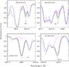 |
Fig. 1 Observed spectrum (dotted lines) for the star #34029 and spectral syntheses for Pb, Y, and Zr. Best fit (red lines) and errors (blue and green lines) are shown, along with syntheses with logϵ(X) ≈ −∞ (magenta). |
Abundances for the Sun and Arcturus.
Abundances for our sample stars.
2.3. Optimisation and tests of the line lists
As first step, we optimised our line lists for all transitions in the solar spectrum (Kurucz et al. 1985); the adopted abundances for the Sun are listed in Table 3. Subsequently, we analysed the Arcturus (α Bootes) spectrum4, given the similarities of this star’s atmospheric parameters to those of our ω Cen giants. Adopted parameters for Arcturus were taken from Fulbright et al. (2007), namely Teff = 4280 K, log g = 1.55, ξ = 1.61 km s-1, and [Fe/H] = −0.50. Our derived abundances are reported in Col. 3 of Table 3, where we also listed results from S00 (Col. 4).
Referring to Table 3, we derive for Arcturus [X/H] = −0.5 for both Y and Zr, −0.60 for La, −0.80 for Ce, and − 0.4 for Eu. If we accept the Fulbright et al. (2007) [Fe/H] value, then [Y/Fe] = [Zr/Fe] = 0.0, [La/Fe] = −0.1, [Ce/Fe] = −0.3, and [Eu/Fe] = + 0.1. It is difficult to compare our abundances with those of major past analyses of Arcturus, because essentially all of them concentrated on the yellow-red spectral regions, and because they were published prior to the recent re-evaluation of transition data for many of the n-capture species considered here. With these cautions, note that some significant study-to-study scatter has been reported. For example, Norris & Da Costa (1995) suggested that the Arcturus relative abundance of all n-capture were essentially all the same, i.e. [n-capture/Fe] = −0.3. Peterson et al. (1993) derived [Y/H] = −0.5 and [Zr/H] = −0.6, in good agreement with our values. However, their abundances for the heavier n-capture elements average about 0.3 dex larger than ours, as they obtained [La/H] = −0.4, [Ce/H] = −0.5, and [Eu/H] = −0.1. As a final example, S00 found lower values than we did for the lighter n-capture abundances, [Y/H] = −0.8 and [Zr/H] = −0.6, but their heavier n-capture abundances were scattered compared to ours, as they derived [La/H] = −0.6, [Ce/H] = −1.2, and [Eu/H] = −0.3. We conclude that our abundance set for Arcturus is reasonable compared to previous work, and that the definitive study of n-capture abundances in this star has yet to be conducted.
Assuming an [O/Fe] = +0.40 (e.g., Lambert & Ries 1981; Cottrell & Sneden 1986; Peterson et al. 1993), we confirmed that [C/Fe] ratio is approximately solar in Arcturus, as also found in these previous studies. Moreover, our determination of [N/Fe] = +0.4 is only slightly higher than those values reported in the earlier work ([N/Fe] = +0.2 to +0.3).
Abundances from spectral synthesis are mainly affected by two sources of uncertainties: errors owing to the best-fit determination and to the stellar parameters, the last being retrieved from JP10 for all our sample stars. Because most of our features are very strong (near to the saturation part of the curve of growth), this is by far the predominant uncertainty, especially when we have only one feature for each element. These errors are reported in Table 4, where we show our final (average) abundances (see next section). When two spectral lines were available for a particular specie, we adopted the standard deviation from the mean of the two lines (rms) as an error estimate.
Errors caused by stellar parameter uncertainties are dominated by microturbulence (ξ) uncertainties, because the spectral lines under scrutiny are usually very strong. An error in Teff of ± 100 K and in log g of ± 0.30 dex (see JP10) results in a maximum variation of Δ = 0.15 dex for [X/Fe]. When we vary ξ by 0.25 km s-1, this implies a Δ[X/Fe] of 0.25−0.30 dex (depending on the species).
In Figs. 1–3 examples of spectral synthesis are shown for star #34029 for all transitions under analysis. As can be seen in the upper panels of Fig. 1, while the Pb line at 4058 Å suffers from a non-negligible contribution from CH molecular features, the bluer line at 3683 Å provides reliable information on the Pb content of this star. We obtain as best-fit value [Pb/Fe] = 0.40 ± 0.20. We also stress that taking into account the C abundance for this star (see Table 4), we derived the same value of [Pb/Fe] = 0.40 ± 0.20 from the 4058 Å line. In general we can conclude from our analysis that to derive accurate Pb measurements, the employment of the blue line at 3683 Å is needed.
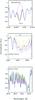 |
Fig. 3 Same as Figs. 1 and 2, but for the [Eu/Fe], CH and CN bands. For the CN bandhead at 4215 a larger spectral window is shown. |
3. Results
3.1. Neutron-capture elements
Our derived abundances are summarised in Table 4, where we list in column 1 the Leiden stellar names, in Cols. 2–9 the [X/Fe] ratios along with their internal uncertainties (see Sect. 2.2), and in Col. 10 the CNO abundance sums. As pointed out by JP10, and as evident in Tables 1 and 4, there is a slight dependence of metallicity (and abundances in general) on Teff values, with the most metal-rich stars being mainly characterised by lower temperature values. The average Teff for stars with [Fe/H] ≤ − 1.28 is 4289 K (rms = 184), while for the more metal-rich stars it is 4127 K (rms = 260), resulting in a difference of 162 K.
In Fig. 4 our derived n-capture abundances [X/Fe] are plotted against [Fe/H] metallicity. For comparison, we also include Y, Zr, and Ce abundances from S00, and La abundances from JP10. With few exceptions the results from the three independent studies are in agreement. In our sample there is a metallicity gap of 0.3 dex at the low end, with four stars having [Fe/H] < −1.7 and the remaining eight stars with [Fe/H] > −1.7. In the discussion below we will contrast these two groups, referring to the relatively metal-rich ones as those with [Fe/H] > −1.7.
First consider the lighter n-capture elements Y and Zr. We observe a substantial change with metallicity in the abundances derived from Y ii and Zr ii lines, as can be seen in the upper two panels of Fig. 4. Indeed, for [Fe/H] ≳ − 1.7, [Yii/Fe] and [Zrii/Fe] appear to suddenly increase by more than a factor of four, reaching maximum values of 1.0 and 1.5, respectively at the highest ω Cen metallicities. The average value of ⟨ [Yii, Zrii/Fe] ⟩ in the four most metal-poor stars is + 0.1, while in stars with [Fe/H] > −1.7 it is + 0.8, i.e. an increase of of 0.7 dex. These increases in [Y, Zr/Fe] are far beyond variations that could be attributed to observational/analytical uncertainties.
Somewhat smaller increases in the relative Y and Zr abundances (~0.5 dex) with increasing metallicity were reported by S00. First, it should be noted that the metallicity ranges of their study is somewhat different from ours. That is, S00 have nine stars out of 10 with [Fe/H] < −1.3, and just one at [Fe/H] ~ −1 dex, while our sample includes seven out of 12 with [Fe/H] ≳ − 1.3 and five more metal-rich than −1.0. This metallicity mismatch makes direct comparison of the variation very difficult, and the big changes in Y and Zr become more apparent above [Fe/H] ~ −1.5, where our sample has more representatives. Additionally, S00 performed an equivalent width (EW) analysis on red Y ii and Zr ii lines, which are extremely weak, with typical values of only a few mÅ and hence may be more affected by measurement uncertainties than our stronger transitions. However, both our sample (12 stars) and the S00 one (10 stars) are quite small and there is no evidence in the literature that the star-to-star scatter in these elements is small within a metallicity bin in ω Cen. A more robust estimation of the trends of these elements with metallicity awaits an attack on larger samples of cluster members distributed over the whole ω Cen metallicity range.
Turning to the heavier n-capture elements, in the middle left panel of Fig. 4 we display [Laii/Fe] values from this work along with those from S00 and JP10. Although the three studies have used different instrumental setup(s), spectral features, and abundance codes, there is an excellent agreement between our study and the others, ignoring one very discrepant high-La, low-metallicity star from S00. Moreover, as also noted by JP10, our lower La abundances with respect to S00 may reflect to a certain extent the lack of the hyperfine structure inclusion in that study. The effect is particularly relevant at higher metallicity, where La ii lines become stronger and “suffer” the effects of the hyperfine structure to a major degree.
Our Ce abundance trend with ω Cen metallicity (middle panel of Fig. 4) excellently agree with that of La. Generally the Ce abundances of S00 agree with ours at similar metallicities, even though these authors’ study had to rely on one weak Ce ii line at 6052 Å. To see the relationship between Ce and La more clearly, we correlate in Fig. 5 [Ce/Fe] with [La/Fe]. Clearly, these elements vary in step within observational uncertainties, over 1 dex ranges in both metallicity and relative abundance. This is a sensible result: in material created by the s-process, La and Ce should share a similar abundance trend, and the s-process fraction of Ce in the solar system material (i.e. 81%) is even higher than La, which has 65%. Note that in Fig. 4 the three most metal-poor stars may have slightly underabundant Ce abundances. The n-capture elements in lower-metallicity ω Cen stars probably have been generated in substantial quantities both by the s-process and the r-process, so a perfect Ce − La correlation over the entire metallicity range should not be expected.
The decreasing contribution of the r-process to the n-capture abundances with increasing metallicity is evident in the bottom left-hand panel of Fig. 4, which displays the run of [Eu ii/Fe] with [Fe/H]. Eu is the most easily observed r-process-dominant element, with a solar-system s-process contribution of only 3% to its total abundance (e.g. Simmerer et al. 2004). The most metal-poor ω Cen stars have [Eu/Fe] ≈ + 0.3, a typical value for globular cluster stars. But [Eu/Fe] ~ 0.0 at the highest metallicities, a trend clearly opposite to that of the previously discussed n-capture elements5. To emphasise this change in nucleosyntic dominance, in Fig. 6 we have constructed s-/r-process abundance surrogates by plotting [X/Eu] ratios versus metallicity for Y, Zr, La, Ce, and Pb. The trends displayed in each panel are qualitatively similar; these five elements appear to have the same s-process nucleosynthetic origin.
The average value of ⟨ [La ii, Ce ii/Fe] ⟩ for stars with [Fe/H] > −1.7 is 0.57, while for the four metal-poor stars it is 0.05, i.e. a variation of ≈0.5 dex. As can be clearly seen from Fig. 7, we found evidence that light-s elements (first-peak) are produced more efficiently than the heavy (second-peak) ones.
S00, on the basis of their data, concluded the opposite; but because they used have a narrower metallicity range and somewhat lower quality data, their conclusion may be affected and our result seems more robust.
The run of [Pb/Fe] as a function of [Fe/H] is shown in the bottom right-hand panel of Fig. 4. While in the two most metal-poor stars only an upper limit to the Pb abundance can be derived, we detected Pb lines in all stars with [Fe/H] ≳ − 1.75. The distribution resembles those of [La/Fe] and [Ce/Fe] shown in the middle panels in Fig. 4. Our derived trends of La, Ce, and Pb with metallicity also are in agree with the [La/Fe] and [Ba/Fe] trends shown by JP10 and M11, i.e., an increase in relative n-capture element abundances beginning at [Fe/H] ~ −1.7/−1.6.
In our ω Cen sample, the ratios [La/Fe], [Ce/Fe], and [Pb/Fe] remain roughly flat at metallicity higher than [Fe/H] ~ −1.5 dex. Considering the two upper limits as measurements, we found a linear correlation coefficient r = 0.69, with a significance level >99%, comparing the trends of Pb with La, Ce. Thus the rise of the s-process in ω Cen includes elements over the whole n-capture domain, from Y (Z = 39) at least up to Ce (Z = 58), and possibly up to Pb (Z = 82). Only the main component of the s-process can yield products over such a wide atomic number (mass) range. This argues against dominance by the weak s-process component; it may have contributed to the overall increase in n-capture abundances with metallicity, but the major effect almost certainly arises from the main component.
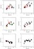 |
Fig. 4 Run of [X/Fe] ratios vs [Fe/H] for Y ii and Zr ii (upper panels), La ii and Ce ii (middle panels), Pb i and Eu ii (lower panels). Triangles are data from S00, while empty squares are for La estimates from JP10. |
3.2. The C+N+O sum
In Table 4 we report our results for C and N abundances as derived from the CH and CN bands, and in Fig. 8 we illustrate the trends of these elements with other abundance quantities. For our complete sample we obtained an average value of [C/Fe] = −0.51 ± 0.10 (rms = 0.33), which agrees very well with previous estimates (e.g. Norris & Da Costa 1995; see also JP10 who adopted that value). However, one star, i.e. #44462, has an anomalously high C abundance. In all four panels of Fig. 8 this star is labelled with a star symbol, because it clearly has not experienced the same chemical history as our other ω Cen giants. The [C/Fe] ratio for this star is more than 10 times (or 2.5σ) higher than the average value of the other 11 stars. The high C content of #44462 is illustrated in Fig. 9 with a small part of the CH G-bandhead. Together with the observed spectrum, synthetic spectra with different [C/Fe] values ([C/Fe] = −1, −0.5, +0.4, and +0.7) are plotted. The figure demonstrates that [C/Fe] = −0.6 (the average value of our complete sample; see below) fails in reproducing the observed CH features of #44462: the best fit for this star is [C/Fe] = + 0.4.
Star #44462 does not stand apart from other stars of its metallicity domain in its total n-capture content. For example, consider stars #34029 ([Fe/H] = −1.28; Table 1) and #60066 ([Fe/H] = −0.98), whose metallicities surround #44462 ([Fe/H] = −1.18). From simple means of the abundances given in Table 4 for the s-process elements Y, Zr, La, Ce, and Pb, we obtain [s-process/Fe] = + 0.59 for #34029, + 0.67 for #44462, and + 0.94 for #60066. These mean values appear to vary directly with [Fe/H], as we have shown above, but are insensitive to [C/Fe]. However, the lighter n-capture elements (Y, Zr) are far more overabundant than the heavier ones (La, Ce) in #44462 relative to the comparison stars (indeed, to any other star of our ω Cen sample). Therefore whatever process produced the very high [C/Fe] ratio in #44462 apparently yielded no contribution to its heavier n-capture elements. Detailed nucleosynthetic arguments on the history of this star are beyond the scope of this paper.
The simplest suggestion for #44462 is that it could have been part of a binary system where the donor star was an AGB, which detached only after a few episodes of the third dredge-up. To search for possible binarity of #44462, we looked for extant radial velocity information. This star was previously analysed by Mayor et al. (1997) and Reijns et al. (2006), who derived vrad = 238.09 ± 0.27 km s-1 and 236.5 ± 1.1 km s-1, respectively. From our spectra we found vrad = 230 ± 1 km s-1. This is suggestive of radial velocity variability, but additional spectroscopic monitoring of this star will be needed to put more firm constraints on this issue.
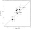 |
Fig. 5 [Ce/Fe] as a function of [La/Fe]. The solid line is a 1:1 relation. |
Discarding this “mild” carbon-star6, we obtained an average of [C/Fe] = −0.59 ± 0.04 (rms = 0.16). Our estimate excellently agree with the value derived for metal-poor (−2 < [Fe/H] < −1) field giants studied by Gratton et al. (2000): the average carbon-to-iron abundance for stars on the upper RGB (i.e. more luminous than the RGB-bump) is [C/Fe] = −0.58 ± 0.03 (rms = 0.12).
Once a C abundance was determined for each star, we adopted its value to derive the CN product from the strong violet band at 4215 Å. As can be seen in Fig. 8 (right upper panel), we found that while low-metallicity stars can be either N-rich or N-poor stars, the most metal-rich ones are all N-rich. For stars with [Fe/H] ≳ −1.4 (with a sharp dependence also on temperature), only lower limits can be provided for nitrogen abundances, because the CN bandhead becomes strongly saturated. Given that our spectra did not include the forbidden [O i] line at 6300 Å (or the permitted triplet, which is too weak in giants however) we could not derive oxygen abundances. Therefore, we adopted O values from JP10. On the basis of our N measurements we confirm that a clear N−O anticorrelation is observable for ω Cen giants, with the exception of the most metal-rich stars (see also M11, JP10). The C+N+O sum as a function of [Fe/H] is shown in the bottom panel (right-hand side) of Fig. 8. We see a moderate rise of this sum up to [Fe/H] ~ −1.5, and then the C+N+O values remain constant at higher metallicity. This again recalls the imprinting of low-mass AGB contribution (see e.g., Busso et al. 1999 and references therein) to intra-cluster pollution, along with the more massive stars that usually are responsible for internal chemical enrichment in GCs.
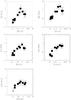 |
Fig. 6 Run of [X/Eu] with [Fe/H] for Y, Zr, La, Ce, and Pb. |
4. Discussion
As discussed in the previous sections, we found that the ratio of light s-process element (Y, Zr) over the heavy s-process ones (La, Ce) is notably shifted towards the first one. However, to obtain a robust evidence of enrichment mechanisms and timescales and to discuss on more quantitative grounds the implications of our results, the computation of the [hs/ls]7 ratio is needed. That is, for all the neutron-caption elements, the r-fraction contribution has to be removed to allow insights into the s-process nucleosynthesis and the involved mass range, and the contamination from different production site(s) has to be derived.
Adopted r/s fractions for n-capture elements.
To do this, we adopted for Y, Zr, La, Ce, Eu, the s- and r-fractions listed in Sneden & Parthasarathy (1983), while for Pb we chose values given by Plez et al. (2004, see Table 5). We proceeded as follows. First, we assumed that [Eus/Las] ≃ [Eus/Las]⊙ for all our sample stars, i.e. the ratio of s-components of Eu and La is solar, because these elements are close to each other in the neutron-capture chain. This is a reasonable assumption because the same s-nucleosynthesis for elements with similar neutron numbers should be expected. We then derived for each element of each star the s-process contribution to the total abundance. The first consideration is that, as also noted by several authors (e.g., Truran 1981; S00; JP10; M11), the most metal-poor stars have a composition dominated by the r-process. This means that even when we deal with species that in the Sun are mainly produced by the s-process (e.g., La, which in the solar system is 35% r-process and 65% s-process), the heavy-element nucleosynthesis is mostly r-process in metal-poor stars. As an example, the metal-poor star #16015 ([Fe/H] = −1.92) has an A(La) = −0.820 ([La/Fe] = −0.03, see Table 4), of which only ~10% should come from s-process production, i.e. A(La)s = −1.838. Thus, to match the condition [Eus/Las] ≃ [Eus/Las]⊙, when the nucleosynthesis is markedly r-process type, these stars cannot be considered in the [hs/ls] plane, because their ratios are not genuine tracers of elements produced by AGB stars and even small errors in abundances cause large uncertainties in the estimated s-fraction.
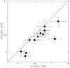 |
Fig. 7 Average values for Y ii and Zr ii as a function of average La ii and Ce ii abundances. |
In Fig. 10 we show the [Pb/ls] ratio as a function of [hs/ls] for all our sample stars whose neutron-capture element pattern is predominantly s-process. Excluding the anomalous C-rich star #44462 discussed above, there is a very clear positive correlation in the [Pb/ls] vs. [hs/ls] diagram. As expected, the variation of [Pb/ls] is roughly a factor of two larger than the one [hs/ls]: this simply reflects the proximity of first- and second-peak elements. The Pb variation evident in Fig. 10 appears to rule out dominant contributions from the weak component to generation of the total s-process pattern observed in ω Cen: the main component clearly is at work here. The suggestion of constant [Cu/Fe] as a function of [Fe/H] (e.g., Cunha et al. 2002) also converges towards the same conclusion. Moreover, theoretical studies (e.g. Raiteri et al. 1992; Pignatari & Gallino 2008) argue that the weak component cannot produce a significant amount of elements heavier than Y, Zr at low metallicity (see references therein for details).
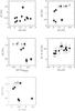 |
Fig. 8 Upper panels: [C/Fe] and [N/Fe] vs. the iron content. The N-O and C-N planes are shown in the left middle and left lower panels, respectively. Our results on the C+N+O sum is displayed in the right middle panel. The star #44462 is denoted by a star symbol (see text). |
Most tantalising is that, because the variation with metallicity of ls elements is larger than the hs ones, the neutron exposures should be quite small; this implies few thermal pulses and larger masses. The s-process seen in ω Cen is clearly different from the standard “Galactic-like” main component, which is predicted to arise from a mass range of donor stars ≈ 1–3.5 M⊙. These AGB stars should yield an over-production of hs with respect to ls in stars with metallicities similar to the ω Cen ones. In Fig. 11 the run of [hs/ls] ratio with metallicity is shown for field stars (open squares, Ba for [hs] and Y for [ls] are from Venn et al. 2004, and references therein) and ω Cen: as is clear from the plot, the [hs/ls] values for cluster giants are lower than in field stars at the same metallicity, indicating an over-abundance of light s-process elements with respect to the heavier ones. For a qualitative comparison, because systematic offsets between theoretical yields and observations can be present, we also show the 3 M⊙ (solid curve) and 1.5 M⊙ (dashed curve) AGB models by Cristallo et al. (2009)8. We note that, discarding the peculiar carbon star #44462, the increasing [hs/ls] ratios occurring at [Fe/H] ≈ −1 dex are well reproduced by the 3 M⊙ AGB model, while the 1.5 M⊙ curve exhibits an opposite (declining) run. Additionally, the expected difference between the two models (~0.2 dex) agrees well with the average difference among ω Cen and field stars.
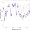 |
Fig. 9 Spectral synthesis for the peculiar star #44462 around the CH G-band at 4300 Å. The continuous line is for the observed spectrum, while dotted lines are for the best fit at [C/Fe] = +0.4. [C/Fe] = −1 (dot-dashed), − 0.5 (short-dashed), and +0.7 (long-dashed) are also shown. |
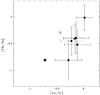 |
Fig. 10 [Pb/ls] as a function of the [hs/ls] ratio (see text for discussion). |
We therefore think that our data reveal the fingerprint of a “peculiar” main component, biased towards the upper end of the mass range of stars involved in the main s-process. The observational clue achieved from the s-process elements is further confirmed by the C+N+O sum, which only slightly increases with metallicity, indicating that only stars with a limited number of third dredge-up episodes contributed to intra-cluster pollution.
While a quantitative estimate of the mass range requires modelling of AGB stars, we tentatively identify stars with mass ≳3 M⊙ as responsible for the s-process production. We do not need to invoke an age spread of one Gyr or more (as would be required from the evolution of ≈ 1.5 M⊙ AGBs) for the later generations in ω Cen. Because ≈3–4 M⊙ AGB stars do evolve in several hundred Myr, a drastic reduction in the age difference of the various stellar populations in ω Cen is then suggested. Recently, D’Antona et al. (2011) concluded that the age spread in ω Cen populations can be at most a few ~108 yr (see also Sollima et al. 2005b), but to reconcile their predictions with the observed s-process pattern, an unknown site of s-process element production has to be invoked. D’Antona et al. advanced the hypothesis that carbon-burning shells of the low-mass tail of the SN II progenitors could be that production site, referring to the study by The et al. (2007). However, these authors pointed out that massive stars (at the final stages of their lives) contribute at least for 40% to s-nuclei with mass A ≤ 87, but only for ~7% (on average) for heavier nuclei (i.e. A > 90). The detected Pb variation hence seems to contradict this scenario, suggesting again that the main s-process component must be a significant mechanism in producing the ω Cen n-capture element mix.
We note that our results do not critically depend on precise values of the r/s fractions adopted in the computation of the [hs/ls] ratios. For instance, we used for the Pb s-fraction the value of 98% provided by Plez et al. (2004), who stressed, however, that the fraction of Pb produced by the r-process in the solar system is practically unknown. Had we instead adopted the 81% given by Simmerer et al. (2004), our results would not have suffered a significant change.
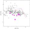 |
Fig. 11 Run of the [hs/ls] ratio as a function of [Fe/H] for field stars (both thick disk and halo, Venn et al. 2004) and ω Cen giants (filled symbols). The solid and dashed curves are for 3 M⊙ AGB and 1.5 M⊙ AGB models from Cristallo et al. (2009), respectively. |
In the derivation of [hs/ls] ratios we used the second-peak elements La and Eu as proxies for the s and r fractions. We checked also if the r/s fractions of the n-capture elements could be confirmed with just a sensitive first-peak element ratio, e.g. [Rb/Zr]. Rb is a good r-process indicator, because it has a substantial r-process component in solar-system material. Rb i has only one transition at 7800 Å, thus we have the correct spectral coverage only for two of the most metal-rich stars, namely #60066 and #60073. However, owing to the low S/N, it was not possible to derive a reliable [Rb/Fe] for star #60066, so we just inspected the trend of #60073. As previously done for Eu and La, we assumed that also [Rbs/Zrs] ≃ [Rbs/Zrs]⊙: for this star we obtained the same fraction of s-process and r-process for each element as the one obtained from the second-peak element ratios.
In the final remarks of their Sect.4.4, S00 compared the [Rb/Zr] ratio (as a tracer of the neutron density environment, see their work for details) with AGB models of 1.5 M⊙, 3 M⊙, and 5 M⊙, with different masses of the 13C pocket (Gallino et al. 1998; Busso et al. 1999). Their plots show that all 5 M⊙ AGB models fail in reproducing the observed abundance pattern: this means that the 22Ne(α, n)25Mg reaction, activated in AGB with masses ≳ 5 M⊙, cannot be invoked as responsible for the s-process production. This idea has been recently advanced also by M 11. In the attempt to reconcile timescale problems, M 11 proposed either an s-process production through the weak component, or intermediate-mass AGBs providing neutrons through 22Ne (see also D’Antona et al. 2011). If stars with mass ≳ 5 M⊙ were neutron-capture element producers, then a quite close relationship should exist between s-process elements and hot H-burning products (e.g., N). Owing to the smallness of our sample, we cannot draw significant conclusions from our data (recall that at [Fe/H] > −1.5, all our sample stars are N-rich), but we refer the reader to Gratton et al. (2011) for a discussion on the complex run of [O/Na] with [La/Fe], based on the extensive dataset from JP10.
Our findings instead agree better with the S00’s view that variations in s-process elements in ω Cen are caused by lower-mass AGBs. Those authors concluded indeed that the best fit to their observations was provided by the lower masses, i.e. 1.5 M⊙, while our conclusions converge towards higher masses. However, we caution the reader again that from their Fig. 14 only the most metal-poor stars, which should have a more markedly r-process pattern however, can be satisfactorily reproduced by the lower-mass AGB model. For stars with [Fe/H] ≥ −1 (where the s-process is predominant) the 3 M⊙ model seems to provide a better agreement. Unfortunately, because we could derive the Rb abundances for only one star, we cannot build up a similar diagram to that given by S00. For star #60073 we found [Rb/Zr] = −0.65 ([Rb/Fe] = 0.05 ± 0.05), which agrees well with the 3 M⊙ AGB model. Remember that the comparison of abundances vs. AGB models cannot be conclusive, because theoretical models strongly depend on a free parameter, i.e. the 13C pocket mass. However, although on the basis of only one star, we suggest that intermediate-mass AGB stars (5–8 M⊙) would result in an overproduction of Rb with respect to Zr (Garcia-Hernandez et al. 2006, and references therein), which is not observed. Once again, this evidence agrees with the previous ones: relatively low-mass AGBs appear to have been responsible for the s-process element enrichment in ω Cen.
5. Conclusions
We presented abundances for a sample of 12 red giants in the peculiar globular cluster ω Cen. We derived light s-process elements (Y, Zr), heavy s-process elements (La, Ce), the r-process element Eu, and for the first time we measured Pb abundances in this cluster. As a complementary information we also obtained abundances for C and N and we computed the C+N+O sum (retrieving O values from JP10).
We detected an indication for Pb production, occurring at [Fe/H] ≳ −1.6: this result allows us to discard the weak component from massive stars as the dominant mechanism for n-capture production in ω Cen. Moreover, from computed [hs/ls] ratios, we conclude that light s-process elements (Y, Zr) vary more than the second-peak ones (La, Ce).
On more general grounds, we suggest that the main s-process component active in ω Cen tends towards the higher mass, ≳3.0 M⊙, notably reducing enrichment timescales from several Gyr, as needed in the case of 1.2−1.5 M⊙ AGBs, to only hundreds million years.
Finally, we note that the acquisition of a more comprehensive sample of ω Cen stars is of paramount importance to draw definite conclusions on these issues. The difference in abundances between our study and the one by S00 might not be entirely caused by the analysis, and a real scatter at any metallicity bin could be present. Accurate heavy-elements abundance estimates for a larger number of stars could allow us to understand both the run of the s-process elements with iron and the presence (if any) of an internal variation.
Elements heavier than iron are mainly synthesised in neutron-capture reactions, which can be divided into s(low)-process and r(apid)-process, where slow and rapid refers to the β-decay timescale.
IRAF is the Image Reduction and Analysis Facility, a general purpose software system for the reduction and analysis of astronomical data. IRAF is written and supported by the IRAF programming group at the National Optical Astronomy Observatories (NOAO) in Tucson, Arizona. NOAO is operated by the Association of Universities for Research in Astronomy (AURA), Inc. under cooperative agreement with the National Science Foundation.
We could not derive Sr abundances because Sr ii features are too heavily saturated in the spectra of our cool red giant sample stars, and our spectra do not include the Sr i line at 4607 Å.
Available at ftp://ftp.noao.edu/catalogs/arcturusatlas/
JP10 determined [Eu/Fe] only for two out of our 12 sample stars, namely #48323, #34180: analysing the 6645 Å feature, they obtained [Eu/Fe] = −0.08 and +0.27 dex, respectively. While for star #48323 their value agrees very well with our measurement, i.e. [Eu/Fe] = −0.10, we found a lower value for star #34180, namely [Eu/Fe] = 0.00. A more detailed study of Eu abundances from multiple transitions in many ω Cen stars should be undertaken.
Note that the C/O ratio is not ≳1 as the formal definition of a carbon star requires.
hs is for heavy s-process elements (second-peak, here La and Ce), and ls is for the lighter ones (first-peak, here Y and Zr). Lead (third-peak) is considered separately.
Available at http://fruity.oa-teramo.inaf.it:8080/modelli.pl
Acknowledgments
This publication made extensive use of the SIMBAD database, operating at CDS (Strasbourg, France) and of NASA’s Astrophysical Data System. This work was partially funded by the Italian MIUR under PRIN 20075TP5K9 and by PRIN INAF “Formation and Early evolution of Massive star clusters”. We thank Marco Pignatari for illuminating discussions on the AGB nucleosynthesis. Financial support to C.S. from the US National Science Foundation through grant AST-0908978 is gratefully acknowledged. We thank the anonymous referee for her/his very helpful suggestions and comments.
References
- Anderson, J. 1998, Ph.D. Thesis, Univ. California, Berkeley [Google Scholar]
- Aoki, W., Ryan, S. G., Norris, J. E., et al. 2002, ApJ, 580, 1149 [NASA ADS] [CrossRef] [Google Scholar]
- Armosky, B. J., Sneden, C., Langer, G. E., & Kraft, R. P. 1994, AJ, 108, 1364 [NASA ADS] [CrossRef] [Google Scholar]
- Barbuy, B., Zoccali, M., Ortolani, S., et al. 2009, A&A, 507, 405 [NASA ADS] [CrossRef] [EDP Sciences] [Google Scholar]
- Bedin, L., Piotto, G., Anderson, J., et al. 2004, ApJ, 605, L125 [NASA ADS] [CrossRef] [Google Scholar]
- Bellazzini, M., Ibata, R. A., Chapman, S. C., et al. 2008, AJ, 136, 1174 [Google Scholar]
- Bellini, A., Bedin, L. R., Piotto, G., et al. 2010, ApJ, 140, 631 [Google Scholar]
- Biémont, E., Garnir, H. P., Palmeri, P., Li, Z. S., & Svanberg, S. 2000, MNRAS, 312, 116 [NASA ADS] [CrossRef] [Google Scholar]
- Bragaglia, A., Sneden, C., Carretta, E., Gratton, R. G., & Lucatello, S. 2011, ApJ, submitted [Google Scholar]
- Busso, M., Gallino, R., & Wasserburg, G. J. 1999, ARA&A, 37, 239 [NASA ADS] [CrossRef] [Google Scholar]
- Carretta, E., Bragaglia, A., Gratton, R. G., et al. 2009a, A&A, 505, 117 [NASA ADS] [CrossRef] [EDP Sciences] [Google Scholar]
- Carretta, E., Bragaglia, A., Gratton, R. G., & Lucatello, S. 2009b, A&A, 505, 139 [NASA ADS] [CrossRef] [EDP Sciences] [Google Scholar]
- Carretta, E., Gratton, R. G., Lucatello, S., et al. 2010b, ApJ, 722, L1 [NASA ADS] [CrossRef] [Google Scholar]
- Carretta, E., Bragaglia, A., Gratton, R. G., et al. 2010c, A&A, 520, A95 [NASA ADS] [CrossRef] [EDP Sciences] [Google Scholar]
- Carretta, E., Lucatello, S., Gratton, R. G., Bragaglia, A., & D’Orazi, V. 2011, A&A, 533, A69 [NASA ADS] [CrossRef] [EDP Sciences] [Google Scholar]
- Catelan, M. 1997, ApJ, 478, L99 [NASA ADS] [CrossRef] [Google Scholar]
- Chiappini, C., Frischknecht, U., Meynet, G., et al. 2011, Nature, 474, 666 [NASA ADS] [CrossRef] [Google Scholar]
- Cohen, J. G. 1999, AJ, 117, 2434 [NASA ADS] [CrossRef] [Google Scholar]
- Cottrell, P. L., & Sneden, C. 1986, A&A, 161, 314 [NASA ADS] [Google Scholar]
- Cristallo, S., Straniero, O., Gallino, R., et al. 2009, ApJ, 696, 797 [NASA ADS] [CrossRef] [Google Scholar]
- Cunha, K., Smith, V. V., Suntzeff, N. B., et al. 2002, AJ, 124, 379 [NASA ADS] [CrossRef] [Google Scholar]
- Decressin, T., Meynet, G., Charbonnel, C., Prantzos, N., & Ekström, S. 2007, A&A, 464, 1029 [NASA ADS] [CrossRef] [EDP Sciences] [Google Scholar]
- D’Antona, F., D’Ercole, A., Marino, A. F., et al. 2011, ApJ, 736, 5 [NASA ADS] [CrossRef] [Google Scholar]
- de Mink, S. E., Pols, O. R., Langer, N., & Izzard, R. G. 2009, A&A, 507, L1 [NASA ADS] [CrossRef] [EDP Sciences] [Google Scholar]
- Denisenkov, P. A., & Denisenkova, S. N. 1989, A. Tsir., 1538, 11 [NASA ADS] [Google Scholar]
- de Silva, G. M., Gibson, B. K., Lattanzio, J., & Asplund, M. 2009, 500, 25 [Google Scholar]
- D’Orazi, V., Gratton, R. G., Lucatello, S., et al. 2010, ApJ, 719, L213 [NASA ADS] [CrossRef] [Google Scholar]
- Ferraro, F. R., Sollima, A., Pancino, E., et al. 2004, ApJ, 603, L81 [NASA ADS] [CrossRef] [Google Scholar]
- Fulbright, J. P., McWilliam, A., & Rich, R. M. 2007, ApJ, 66, 1152 [NASA ADS] [CrossRef] [Google Scholar]
- Gallino, R., Arlandini, C., Busso, M., et al. 1998, ApJ, 497, 388 [NASA ADS] [CrossRef] [PubMed] [Google Scholar]
- Garcia-Hernandez, D. A., Garcia-Lario, P., Plez, F., et al. 2006, Science, 314, 1751 [NASA ADS] [CrossRef] [Google Scholar]
- Gratton, R. G. 1985, A&A, 148, 105 [NASA ADS] [Google Scholar]
- Gratton, R. G. 1988, Rome Observatory Preprint Ser., 29 [Google Scholar]
- Gratton, R. G., Sneden, C., Carretta, E., & Bragaglia, A. 2000, A&A, 354, 169 [NASA ADS] [Google Scholar]
- Gratton, R. G., Sneden, C., & Carretta, E. 2004, ARA&A, 42, 385 [NASA ADS] [CrossRef] [Google Scholar]
- Gratton, R. G., Carretta, E., Bragaglia, A., Lucatello, S., & D’Orazi, V. 2010, A&A, 517, A81 [NASA ADS] [CrossRef] [EDP Sciences] [Google Scholar]
- Gratton, R. G., Johnson, C. I., Lucatello, S., D’Orazi, V., & Pilachowski, C. 2011, A&A, in press [Google Scholar]
- Han, S.-I., Lee, Y.-W., Joo, S.-J., et al. 2009, ApJ, 707, L190 [NASA ADS] [CrossRef] [Google Scholar]
- Hannaford, P., Lowe, R. M., Grevesse, N., et al. 1982, ApJ, 261, 736 [NASA ADS] [CrossRef] [Google Scholar]
- James, G., François, P., Bonifacio, P., et al. 2004, A&A, 427, 825 [NASA ADS] [CrossRef] [EDP Sciences] [Google Scholar]
- Johnson, C. I., & Pilachowski, C. A. 2010, ApJ, 722, 1373 (JP10) [NASA ADS] [CrossRef] [Google Scholar]
- Kayser, A., Hilker, M., Grebel, E. K., & Willemsen, P. G. 2008, A&A, 486, 437 [NASA ADS] [CrossRef] [EDP Sciences] [Google Scholar]
- Kraft, R. P. 1994, PASP, 106, 553 [NASA ADS] [CrossRef] [Google Scholar]
- Kurucz, R. L. 1993, CD-ROM 13, Cambridge, Mass., Smithsonian Astrophysical Observatory [Google Scholar]
- Kurucz, R. L., Furenlid, I., Brault, J., & Testerman, L. 1985, S&T, 70, 38 [Google Scholar]
- Lambert, D. L., & Ries, L. M. 1981, ApJ, 248, 228 [NASA ADS] [CrossRef] [Google Scholar]
- Langer, G. E., Hoffman, R., & Sneden, C. 1993, PASP, 105, 301 [NASA ADS] [CrossRef] [Google Scholar]
- Lawler, J. E., Bonvallet, G., & Sneden, C. 2001a, ApJ, 556, L452 [NASA ADS] [CrossRef] [Google Scholar]
- Lawler, J. E., Wickliffe, M. E., den Hartog, E. A., & Sneden, C. 2001b, ApJ, 563, 1075 [CrossRef] [Google Scholar]
- Lawler, J. E., Sneden, C., Cowan, J. J., Ivans, I. I., & Den Hartog, E. A. 2009, ApJS, 182, L51 [NASA ADS] [CrossRef] [Google Scholar]
- Lee, T.-W., Joo, J.-M., Sohn, Y.-J., et al. 1999, Nature, 402, 55 [NASA ADS] [CrossRef] [Google Scholar]
- Lind, K., Primas, F., Charbonnel, C., Grundahl, F., & Asplund, M. 2009, A&A, 503, 545 [NASA ADS] [CrossRef] [EDP Sciences] [MathSciNet] [Google Scholar]
- Ljung, G., Nilsson, H., Asplund, M., & Johansson, S. 2006, A&A, 456, 1181 [NASA ADS] [CrossRef] [EDP Sciences] [Google Scholar]
- Marino, A. F., Milone, A. P., Piotto, G., et al. 2009, A&A, 505, 1099 [NASA ADS] [CrossRef] [EDP Sciences] [Google Scholar]
- Marino, A. F., Milone, A. P., Piotto, G., et al. 2011, ApJ, 731, 64 (M11) [NASA ADS] [CrossRef] [Google Scholar]
- Martell, S. L. 2011, AN, 332, 467 [Google Scholar]
- Mashonkina, L. I., Vinogradova, A. B., Ptitsyn, D. A., Khokhlova, V. S., & Chernetsova, T. A. 2007, ARep, 51, 903 [Google Scholar]
- Mayor, M., Meylan, G., Udry, S., et al. 1997, AJ, 114, 1087 [Google Scholar]
- Milone, A. P., Bedin, L., Piotto, G., et al. 2008, ApJ, 673, 241 [NASA ADS] [CrossRef] [Google Scholar]
- Norris, J. E., & Da Costa, G. S. 1995, ApJ, 447, 680 [NASA ADS] [CrossRef] [Google Scholar]
- Origlia, L., Ferraro, F. R., Bellazzini, M., & Pancino, E. 2003, ApJ, 591, 916 [NASA ADS] [CrossRef] [Google Scholar]
- Pancino, E., Ferraro, F. R., Bellazzini, M., et al. 2000, ApJ, 583, L83 [NASA ADS] [CrossRef] [Google Scholar]
- Pancino, E., Pasquini, L., Hill, V., Ferraro, F. R., & Bellazzini, M. 2002, ApJ, 568, L101 [NASA ADS] [CrossRef] [Google Scholar]
- Pancino, E., Origlia, L., Ferraro, F. R., et al. 2003, ASPC, 296, 226 [NASA ADS] [Google Scholar]
- Pancino, E., Carrera, R., Rossetti, E., & Gallart, C. 2010a, A&A, 511, A56 [NASA ADS] [CrossRef] [EDP Sciences] [Google Scholar]
- Pancino, E., Rejkuba, M., Zoccali, M., & Carrera, R. 2010b, A&A, 524, A44 [NASA ADS] [CrossRef] [EDP Sciences] [Google Scholar]
- Pasquini, L., Bonifacio, P., Molaro, P., et al. 2005, A&A, 441, 549 [NASA ADS] [CrossRef] [EDP Sciences] [Google Scholar]
- Peterson, R. C., Dal le Ore, C. M., & Kurucz, R. L. 1993, ApJ, 404, 333 [NASA ADS] [CrossRef] [Google Scholar]
- Pignatari, M., & Gallino, R. 2008, AIPC, 990, 336 [NASA ADS] [Google Scholar]
- Plez, B., Hill, V., Cayrel, R., et al. 2004, A&A, 428, L9 [NASA ADS] [CrossRef] [EDP Sciences] [Google Scholar]
- Raiteri, C. M., Gallino, R., & Busso, M. 1992, ApJ, 387, 263 [NASA ADS] [CrossRef] [Google Scholar]
- Raiteri, C. M., Busso, M., Neuberger, D., & Käppeler, F. 1993, ApJ, 419, 207 [NASA ADS] [CrossRef] [Google Scholar]
- Reijns, R. A., Seitzer, P., Arnold, R., et al. 2006, A&A, 445, 503 [NASA ADS] [CrossRef] [EDP Sciences] [Google Scholar]
- Roederer, I. U. 2011, ApJ, 732, L17 [NASA ADS] [CrossRef] [Google Scholar]
- Roederer, I. U., Kratz, K.-L., Frebel, A., et al. 2009, ApJ, 698, 1693 [Google Scholar]
- Rose, J. L., & Granath, L. P. 1932, Phys. Rev., 40, 760 [NASA ADS] [CrossRef] [Google Scholar]
- Sarajedini, A., & Layden, A. C. 1995, AJ, 109, 1086 [NASA ADS] [CrossRef] [Google Scholar]
- Shen, Z.-X., Bonifacio, P., Pasquini, L., & Zaggia, S. 2010, A&A, 524, L2 [NASA ADS] [CrossRef] [EDP Sciences] [Google Scholar]
- Simmerer, J., Sneden, C., Cowan, J. J., et al. 2004, ApJ, 617, 1091 [NASA ADS] [CrossRef] [Google Scholar]
- Smith, V. V., Suntzeff, N. B., Cunha, K., et al. 2000, AJ, 119, 1239 (S00) [NASA ADS] [CrossRef] [Google Scholar]
- Sneden, C., & Parthasarathy, M. 1983, ApJ, 267, 757 [NASA ADS] [CrossRef] [Google Scholar]
- Sneden, C., Kraft, R. P., Shetrone, M. D., et al. 1997, AJ, 114, 1964 [NASA ADS] [CrossRef] [Google Scholar]
- Sobeck, J. S., Kraft, P. R., Sneden, C., et al. 2011, AJ, 141, 175 [NASA ADS] [CrossRef] [Google Scholar]
- Sollima, A., Ferraro, F. R., Pancino, E., & Bellazzini, M. 2005a, MNRAS, 357, 265 [NASA ADS] [CrossRef] [Google Scholar]
- Sollima, A., Pancino, E., Ferraro, F. R., et al. 2005b, ApJ, 634, 332 [NASA ADS] [CrossRef] [Google Scholar]
- Sollima, A., Ferraro, F. R., Bellazzini, M., et al. 2007, ApJ, 654, 915 [NASA ADS] [CrossRef] [Google Scholar]
- Stetson, P. B. 1981, AJ, 86, 687 [NASA ADS] [CrossRef] [Google Scholar]
- The, L.-S., El Eid, M. F., & Meyer, B. S. 2007, ApJ, 655, 1058 [NASA ADS] [CrossRef] [Google Scholar]
- Travaglio, C., Gallino, R., Arnone, E., et al. 2004, ApJ, 601, 864 [NASA ADS] [CrossRef] [Google Scholar]
- Truran, J. W. 1981, A&A, 97, 391 [NASA ADS] [Google Scholar]
- van de Ven, G., van den Bosch, R. C. E., Verolme, E. K., & de Zeeuw, P. T. 2006, A&A, 445, 513 [NASA ADS] [CrossRef] [EDP Sciences] [Google Scholar]
- van Leeuwen, F., Le Poole, R. S., Freeman, K. C., & de Zeeuw, P. T. 2000, A&A, 360, 472 [NASA ADS] [Google Scholar]
- Venn, K. A., Irwin, M., Shetrone, M. D., et al. 2004, AJ, 128, 1177 [NASA ADS] [CrossRef] [Google Scholar]
- Ventura, P., D’Antona, F., Mazzitelli, I., & Gratton, R. G. 2001, ApJ, 550, L65 [NASA ADS] [CrossRef] [Google Scholar]
- Villanova, S., Geisler, D., & Piotto, G. 2010, ApJ, 722, L18 [NASA ADS] [CrossRef] [Google Scholar]
- Woolley, R. R. 1966, R. Obs. Ann., 2, 1 [Google Scholar]
- Yong, D., & Grundahl, F. 2008, ApJ, 672, L29 [NASA ADS] [CrossRef] [Google Scholar]
All Tables
Identification, photometry, and adopted parameters for our programme stars (see JP10).
All Figures
|
Fig. 1 Observed spectrum (dotted lines) for the star #34029 and spectral syntheses for Pb, Y, and Zr. Best fit (red lines) and errors (blue and green lines) are shown, along with syntheses with logϵ(X) ≈ −∞ (magenta). |
| In the text | |
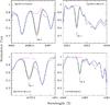 |
Fig. 2 Same as Fig. 1 but for the La and Ce lines. |
| In the text | |
|
Fig. 3 Same as Figs. 1 and 2, but for the [Eu/Fe], CH and CN bands. For the CN bandhead at 4215 a larger spectral window is shown. |
| In the text | |
|
Fig. 4 Run of [X/Fe] ratios vs [Fe/H] for Y ii and Zr ii (upper panels), La ii and Ce ii (middle panels), Pb i and Eu ii (lower panels). Triangles are data from S00, while empty squares are for La estimates from JP10. |
| In the text | |
|
Fig. 5 [Ce/Fe] as a function of [La/Fe]. The solid line is a 1:1 relation. |
| In the text | |
|
Fig. 6 Run of [X/Eu] with [Fe/H] for Y, Zr, La, Ce, and Pb. |
| In the text | |
|
Fig. 7 Average values for Y ii and Zr ii as a function of average La ii and Ce ii abundances. |
| In the text | |
|
Fig. 8 Upper panels: [C/Fe] and [N/Fe] vs. the iron content. The N-O and C-N planes are shown in the left middle and left lower panels, respectively. Our results on the C+N+O sum is displayed in the right middle panel. The star #44462 is denoted by a star symbol (see text). |
| In the text | |
|
Fig. 9 Spectral synthesis for the peculiar star #44462 around the CH G-band at 4300 Å. The continuous line is for the observed spectrum, while dotted lines are for the best fit at [C/Fe] = +0.4. [C/Fe] = −1 (dot-dashed), − 0.5 (short-dashed), and +0.7 (long-dashed) are also shown. |
| In the text | |
|
Fig. 10 [Pb/ls] as a function of the [hs/ls] ratio (see text for discussion). |
| In the text | |
|
Fig. 11 Run of the [hs/ls] ratio as a function of [Fe/H] for field stars (both thick disk and halo, Venn et al. 2004) and ω Cen giants (filled symbols). The solid and dashed curves are for 3 M⊙ AGB and 1.5 M⊙ AGB models from Cristallo et al. (2009), respectively. |
| In the text | |
Current usage metrics show cumulative count of Article Views (full-text article views including HTML views, PDF and ePub downloads, according to the available data) and Abstracts Views on Vision4Press platform.
Data correspond to usage on the plateform after 2015. The current usage metrics is available 48-96 hours after online publication and is updated daily on week days.
Initial download of the metrics may take a while.