| Issue |
A&A
Volume 534, October 2011
|
|
|---|---|---|
| Article Number | A78 | |
| Number of page(s) | 11 | |
| Section | The Sun | |
| DOI | https://doi.org/10.1051/0004-6361/201117416 | |
| Published online | 05 October 2011 | |
Resonant damping of kink oscillations of cooling coronal magnetic loops
Solar Physics and Space Plasma Research Centre (SP 2RC), University of Sheffield, Hicks Building, Hounsfield Road, Sheffield S3 7RH, UK
e-mail: This email address is being protected from spambots. You need JavaScript enabled to view it.
Received: 6 June 2011
Accepted: 16 August 2011
Abstract
The simultaneous effect of amplification due to cooling and damping due to resonant absorption on the kink oscillations of coronal loops is studied. The governing equation describing the kink oscillations is derived in the thin tube thin boundary layer approximation. The cooling time is assumed to be much larger than the oscillation period, and the Wentzel-Kramers-Brillouin (WKB) method is used to obtain the equation describing the dependence of the oscillation amplitude on time. This equation is solved numerically for various values of determining parameters. In particular, the question if the amplification due to cooling can balance the resonant damping and produce undamped oscillation is addressed. The conclusion is that the amplification due to cooling is not very efficient and can balance the resonant damping only when the density contrast is not very large and the cooling is very fast with the characteristic cooling time of the order of the oscillation period.
Key words: magnetohydrodynamics (MHD) / plasmas / Sun: corona / Sun: oscillations / waves
© ESO, 2011
1. Introduction
Transverse coronal loop oscillations were first observed by TRACE in 1998. This observation was reported by Aschwanden et al. (1999) and Nakariakov et al. (1999) who interpreted these oscillations as standing fast kink waves. An important property of these oscillations was that they quickly damped with the characteristic damping time of the order of a few oscillation periods. Ruderman & Roberts (2002) suggested that this damping was due to resonant absorption related to the loop inhomogeneity in the radial direction. Using the thin tube thin boundary (TTTB) approximation they provided the estimate of the loop inhomogeneity using the observed damping time. Later Goossens et al. (2002) obtained similar estimates for eleven events where the coronal loop kink oscillations were observed.
An important property of oscillating coronal loops is that, very often, they are in a highly dynamic state. In particular, they can cool quickly with the characteristic cooling time of the order of a few periods of the kink oscillation (Aschwanden & Terradas 2008). This observation put on the agenda theoretical study of MHD waves and oscillations in dynamic plasmas. Morton et al. (2009) studied propaqation of MHD waves in a homogeneous plasma with parameters varying in time. The effect of cooling on the coronal loop kink oscillations was first studied by Morton & Erdélyi (2009, 2010) who showed that cooling causes the decrease of the oscillation period. Ruderman (2011b, Paper I in what follows) studied the kink oscillations of coronal loops with slowly varying density (note that Figs. 3, 6 and 7 in this paper are incorrected; the corrected figures are given in Ruderman 2011a). He obtained the so-called adiabatic invariant determining the time-evolution of the oscillation amplitude and showed that cooling causes the amplification of kink oscillations.
Although, as we have already mentioned, usually the coronal loop kink oscillations are heavily damped, sometimes it is observed that their amplitude practically does not change during the entire time of observation. In particular, in 17 events of coronal loop kink oscillations reported by Aschwanden et al. (2002) no damping was observed in 7 of these events. Recently Aschwanden & Schrijver (2011) reported observations of coronal loop oscillations using data from Atmospheric Imaging Assembly (AIA) onboard Solar Dynamic Observatory (SDO). In one case the oscillation was practically undamped. Aschwanden & Schrijver (2011) concluded that, if we assume that the damping is due to resonant absorption and use the thin tube thin boundary (TTTB) approximation, then the ratio of the thickness of the transitional layer where the density changes, ℓ, to the loop radius R should be extremely small. An important property of the observed loop was that it was cooling. It was suggested in Paper I that the loop oscillation was undamped because the damping due to resonant absorption was balanced by amplification due to cooling. Then the ratio ℓ/R was estimated. For this it was assumed that the characteristic amplification time is equal to the damping time. For a particular event reported by Aschwanden & Schrijver (2011)ℓ/R ≈ 0.04 was obtained, so, in that case, the conclusion by Aschwanden & Schrijver (2011) that the transition layer has to be extremely thin remains valid. However, it was noted in Paper I that the characteristic amplification time and, as a result, the estimate of ℓ/R, is very sensitive to the cooling time and the initial temperature of the loop.
The method used in Paper I to estimate ℓ/R is not very accurate. The main reason is that it does not take into account the effect of cooling on the damping rate. Cooling causes the average density decrease in the loop and, as a result, the decrease of the ratio of average densities inside and outside the loop. This decrease of the average density ratio affects the damping rate. Hence, the effect of loop cooling on kink oscillations of coronal loops is two-fold: it amplifies the oscillations and affects the damping rate due to resonant absorption.
The aim of this paper is to study the simultaneous effect of cooling and resonant absorption on coronal loop kink oscillations. The paper is organized as follows. In the next section we formulate the problem, introduce the quasi-Lagrangian description, and derive the linear governing equation for the magnetic field line displacement in the cold plasma approximation. In Sect. 3 we derive the general governing equation for kink oscillations of magnetic loops in the thin tube thin boundary (TTTB) approximation. In Sect. 4 we consider oscillations of slowly cooling loops and derive the equation for the oscillation amplitude that describes both the amplification of oscillations due to cooling and their damping due to resonant absorption. In Sect. 5 we study the oscillations of loops with the barometric density variation along the loop. Section 6 contains the summary of the obtained results and our conclusions.
2. Problem formulation and quasi-Lagrangian description
The coronal loop is modelled as a straight magnetic tube with the magnetic field having the same direction and magnitude inside and outside the tube. In what follows we use cylindrical coordinates r, ϕ, z with the z-axis coinciding with the magnetic tube axis. The plasma density ρ is a function of r, z and time t. It varies from its value inside the tube to its value outside in a transitional layer of thickness ℓ. Hence, it is given by 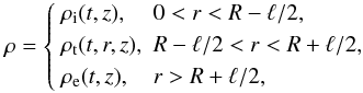 (1)where R is the radius of the loop cross-section and ρt(t,r,z) is a monotonic function of r, ρt(t,R − ℓ/2,z) = ρi(t,z), ρt(t,R + ℓ/2,z) = ρe(t,z). The density variation with time causes the plasma flow in the z-direction. The plasma density and background flow velocity U(t,r,z) are related by the mass conservation equation,
 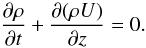 (2)The perturbations of the magnetic field and plasma velocity, b = (br,bϕ,bz) and u = (ur,uϕ,uz), are described by the linearized MHD equations in the cold plasma approximation,
 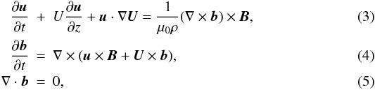 where U = Uez, B = Bez, B = const is the magnetic field magnitude, ez is the unit vector in the z-direction, and μ0 is the magnetic permeability of free space. Dissipation is only important in the dissipative layers embracing Alfvénic resonant magnetic surfaces in the region R − ℓ/2 < r < R + ℓ/2. Since we neglected dissipative terms in Eqs. (3)–(5), these equations describe the plasma motion everywhere except in the dissipative layers. It follows from Eq. (3) that uz = 0.
Now we introduce the so-called quasi-Lagrangian description. Consider an individual magnetic field line. The equation of the unperturbed magnetic field line can be written in the vector form as r = zez + a, where r is the position vector of any point on the magnetic field line, a is a constant vector and a ⊥ ez. The equation of the perturbed magnetic field line is 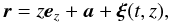 (6)where ξ ⊥ ez is the magnetic field line displacement. Consider a fluid particle that is on this magnetic field line at the initial moment of time. Since the magnetic field is frozen in the plasma the particle will remain on this magnetic field line at any subsequent moment of time. Then its trajectory is given by
  (7)and the velocity by
  (8)Taking into account that uz = 0 we obtain
  (9)The magnetic field vector is tangent to the magnetic field line, which implies that Bez + b is parallel to ez + ∂ξ/∂z. It follows from this relation that, in the linear approximation,
  (10)where b ⊥ = (br,bϕ,0). Substituting Eqs. (9) and (10) in Eq. (4) we find that the perpendicular component of this equation, i.e. the component normal to the z-direction, is satisfied identically.
Let us introduce the perturbation of the magnetic pressure P = Bbz/μ0. To obtain the relation between bz and ξ we use the z-component of Eq. (4) and Eq. (5). Then, using Eqs. (9) and (10), we obtain  (11)where
  is the square of the Alfvén speed. Assuming that
  at the initial moment of time, we arrive at
  (12)Substituting Eqs. (9) and (10) in Eq. (3), taking into account that uz = 0, and using the identity
 which is valid when B = const, yields
  (13)where
 We assume that at the loop foot points the magnetic field lines are frozen in the dense photospheric plasma, so
  (14)where L is the loop length. In what follows Eqs. (12) and (13) together with the boundary conditions (14) are used to study the plasma motion everywhere except the dissipative layers.
3. Derivation of the governing equation
In this section we use Eq. (13) only in the regions r < R − ℓ/2 and r > R + ℓ/2 where ρ is independent of r. We start the derivation of the governing equation from introducing the small parameter ϵ = R/L. For typical coronal loops this parameter does not exceed 0.05. Then we introduce the stretched variable Z = ϵz. Further, we outline that the oscillation period can be considered as the characteristic time of the problem. It is of the order of L/Ckh = ϵ-1R/Ckh, where Ckh is the characteristic kink speed. This estimate inspires us to introduce the “slow” time T = ϵt. Now we apply the operator (∇ ⊥ ·) to Eq. (13). Using Eq. (12) we obtain the equation for P: 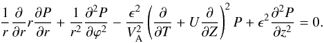 (15)In what follows we consider only kink oscillations and take ξ and P proportional to exp(iϕ). Then, neglecting terms of the order of ϵ2 in Eq. (15) we reduce it to
 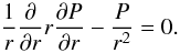 (16)The thin tube approximation cannot be used to describe the plasma motion far from the magnetic tube. However, we only consider the oscillations with the amplitude that rapidly decays with the distance from the tube boundary, so we only need to describe the plasma motion in the immediate vicinity of the tube. Hence, we can use Eq. (16) both inside and outside the tube. The solution to Eq. (16) has to be regular at r = 0 and tend to zero as r → ∞. Using these conditions we obtain
 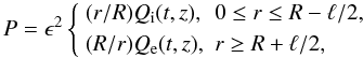 (17)where, at present, Qi(t,z) and Qe(t,z) are arbitrary functions satisfying the conditions Qi(t, ± L/2) = Qe(t, ± L/2) = 0, and the multiplier ϵ2 has been introduced for the convenience. Note that Eq. (17) remains valid even for leaky oscillations (see Dymova & Ruderman 2005). Substituting this equation in Eq. (13) we obtain
 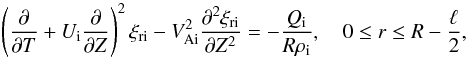 (18)
(18) (19)In particular, it follows from Eqs. (12) and (18) that ξ is independent of r in the region 0 ≤ r ≤ R − ℓ/2.
Let us introduce the jump of function f(r) across the inhomogeneous layer,
 In the following calculations we keep terms proportional to ℓ/R while we neglect terms proportional to (ℓ/R)2 and the higher powers of ℓ/R. It follows from Eqs. (12) and (13) that δξr ~ ℓ/R and δP ~ ℓ/R. Using the second of these estimates and Eq. (17) we obtain the approximate relation
 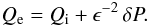 (20)Substituting this result in Eq. (19) we obtain the approximate equation
 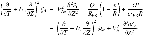 (21)Eliminating Qi from Eqs. (18) and (21) yields
 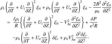 (22)To simplify the notation we introduce η = ξri. Then, returning to the original independent variables, we eventually arrive at
  (23)where
  (24)ℒ = 0 when ℓ = 0. In this case Eq. (23) coincides with Eq. (21) in Ruderman (2010).
4. Kink oscillations of coronal loops with slowly varying density
4.1. The WKB approximation
The aim of this section is to derive the equation governing the time dependence of the amplitude of kink oscillations of coronal loops with slowly varying density in the presence of resonant damping. Let us introduce the notation ν = ℓ/R ≪ 1. We assume that the characteristic time of the density variation, tch, is much larger than the characteristic oscillation period, Pch. We aim to obtain the equation for the amplitude that describes the effects of density variation and resonant damping in the same order approximation. In accordance with this we put  . Now, similar to Paper I, we use the Wentzel-Kramers-Brillouin (WKB) method (see, e.g. Bender & Orszag 1978). In accordance with this method we write
 ![Mathematical equation: \begin{equation} \eta = S(t,z)\exp[{\rm i}\nu^{-1}\Theta(t)]. \label{eq:4.1} \end{equation}](/articles/aa/full_html/2011/10/aa17416-11/aa17416-11-eq93.png) (25)Then we expand S in the series
(25)Then we expand S in the series  (26)It follows from our assumptions that the characteristic period of kink oscillations is νtch. On the other hand, it is also of the order of the loop length divided by the characteristic kink speed. Hence, it can be taken to be equal to
  , where ρch is the characteristic density. As a result we have
 This estimate inspired us to introduce the scaled magnetic field
  . It follows from Eqs. (18) and (19) that Qi,e ~ ν-2, which implies that P ~ ν-2. Since δP/P ~ ν, we have δP ~ ν-1. In accordance with this estimate we introduce the scaled variable
  . Now, substituting Eqs. (25) and (26) in Eq. (23), we obtain
 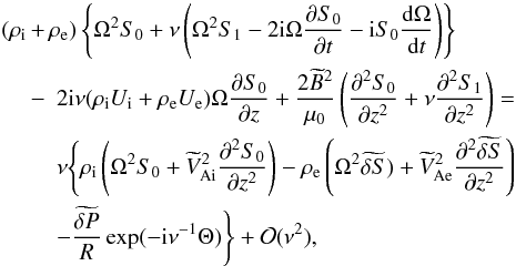 (27)where
  (28)where δS is the jump of S across the transitional layer.
Collecting terms of the order of one in this equation yields 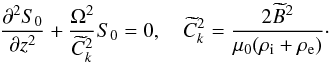 (29)This approximation is sometimes called the approximation of geometrical optics. Introducing
 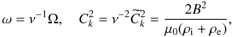 (30)we rewrite Eq. (29) as
 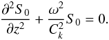 (31)The quantity ω can be considered as the instantaneous frequency of kink oscillation. It follows from Eq. (14) that S0 satisfies the boundary conditions
 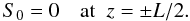 (32)Equations (29) and (32) constitute the boundary value problem that determines the oscillation frequency Ω. This problem coincides with the boundary value problem obtained by Dymova & Ruderman (2005) for kink oscillations of a magnetic tube with the density varying along the tube that is in a static equilibrium. In what follows we assume that Ω2 is the eigenvalue and S0 the corresponding eigenfunction of the boundary value problem defined by Eqs. (29) and (32). In accordance with the general theory of the Sturm-Liouville problem Ω2 is real (see, e.g. Coddington & Levinson 1978). It is straightforward to see that Ω2 > 0.
In the next order approximation, sometimes called the approximation of physical optics, we collect the terms of the order of ν in Eq. (27). With the aid of Eq. (29) this yields 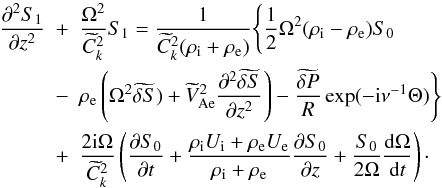 (33)It follows from Eq. (14) that S1 satisfies the boundary conditions
  (34)The homogeneous counterpart of the boundary value problem constituted by Eqs. (33) and (34) has a non-trivial solution S1 = S0. This means that the boundary value problem determining S1 has a solution only when the right-hand side of Eq. (33) satisfies the compatibility condition. We obtain this compatibility condition by multiplying Eq. (33) by S0, integrating the obtained equation, and using the integration by parts and Eq. (34). After some algebra we write this condition as
 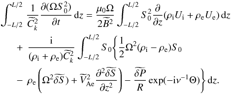 (35)Using the mass conservation Eq. (2) we obtain
 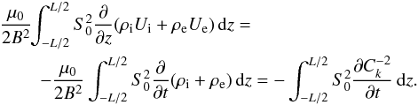 (36)Substituting this expression in Eq. (35) we transform it to
 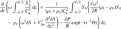 (37)The quantity in the brackets on the left-hand side of this equation is called the adiabatic invariant. When ℓ = 0 the right-hand side of Eq. (37) is zero, the adiabatic invariant is conserved, and Eq. (37) coincides with Eq. (16) in Paper I.
It is worth noting that, even when ℓ = 0, the oscillation energy is not conserved because the cooling loop is an open system. Really, during the cooling the total mass of the loop decreases, so there is the flux of the plasma and, consequently, also the energy flux through the foot points. Hence the conservation of the adiabatic invariant is not related to the energy conservation. Probably it can be interpreted in terms of conservation of the wave action, however this is a problem for the future study.
The equation expressing the conservation of the adiabatic invariant becomes especially simple in the case of a homogeneous coronal loop and the ratio of densities inside and outside the loop independent of time, which was considered in Paper I. In this case ω = πCk/L and it follows from the adiabatic invariant conservation that the wave amplitude is proportional to  .
.
4.2. Calculation of δξr and δP
Equation (37) determines the time evolution of S0 and thus the oscillation amplitude. However this equation is not closed. To make it closed we need to express δS and δP in terms of S0. It follows from Eq. (2) that U is of the order of νCkh. We also have the estimate ∂S0/∂t ~ νωS0. This implies that the account of the flow and the time derivative of S0 in the description of plasma motion in the transitional layer will only give corrections of the order of ν to the expressions for δS and δP. Since we only need to calculate the right-hand side of Eq. (37) in the leading order approximation with respect to ν, it follows that we need to calculate δS and δP also only in the leading order approximation with respect to ν. This implies that we can neglect the plasma flow and the time derivative of S0 and use the quasi-static description of plasma motion in the transitional layer when calculating δS and δP. The only difference between the static and quasi-static description is that, while in the former the coefficient functions in the equations describing the plasma motion are independent of time, in the latter they depend on time as on a parameter. Then we can use the results obtained by Dymova & Ruderman (2006, Paper II in what follows) in the static case. However the analysis in Paper II was carried out under the assumption that ρe/ρi is independent of z. Since we do not make this assumption we have to modify this analysis. In what follows we briefly describe the results obtained in Paper II and the modifications that we make.
First of all we notice that, in Paper II, not the jump of the radial displacement but the jump of the radial velocity across the transitional layer was calculated. However it does not cause any problem because, in the quasi-static description, this jump is just equal to iω δξr. Also notice that, in Paper II, the frequency with the different sign was used. Now, following Paper II, we consider the Alfvén oscillations of individual magnetic field lines. They are described by the eigenvalue problem 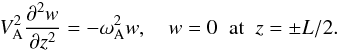 (38)In this equation
  is the square of the Alfvén frequency. Note that VA and w are functions of t, r and z, and is a function of t and r. The eigenvalues of this problem are real and constitute an infinite monotonically increasing sequence
  ,
,  as n → ∞ (see, e.g. Coddington & Levinson 1978). It is straightforward to show that all eigenvalues are positive. Any function g(z) square integrable in the interval [ − L/2,L/2] can be expanded in the generalized Fourier series
 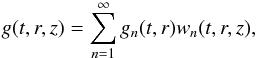 (39)where wn(t,r,z) is the eigenfunction of the boundary value problem (38) corresponding to the eigenvalue
  . Obviously, all wn can be chosen to be real. The eigenfunctions corresponding to different eigenvalues are orthogonal with the weight
  . In addition they can be normalized in such a way that they satisfy the relation
 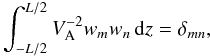 (40)where δmn is the Kronecker delta-symbol. If g(z) has a continuous second derivative and satisfies the boundary conditions g( ± L/2) = 0, then the sum in (39) is uniformly convergent and can be differentiated twice (see, e.g. Titchmarsh 1946; Naimark 1967). The Fourier coefficients are given by
  (41)The global kink oscillation is in resonance with nth harmonic of local Alfvén oscillations at the resonant magnetic surface defined by the equation r = rn if the condition
  is satisfied. Since
  as n → ∞, there can be only a finite number of Alfvén resonances. Observations show that, in most cases, the fundamental harmonic of kink oscillations is dominant, so the oscillation amplitude is determined by the fundamental harmonic. De Moortel & Brady (2007) reported observations of coronal loop kink oscillations where a node was present. This may indicate that the first overtone was the dominant mode in these oscillations. However, De Moortel & Brady (2007) pointed out that there is a possibility that the observed node was a purely geometrical effect related to the fact that the loops were non-planar. Recently this possibility was confirmed in the theoretical study of kink oscillations of non-planar loops by Ruderman & Scott (2011). In accordance with this we consider only the fundamental harmonic of the kink oscillations in what follows.
When ρi(z) > ρe(z) for all z ∈ [ − L/2,L/2] , we have VAi(z) < Ck(z) < VAe(z) for all z ∈ [ − L/2,L/2] . In that case, using the oscillations theorem (e.g. Coddington & Levinson 1978), we can prove that  , which implies that there is r1 ∈ [R − ℓ/2,R + ℓ/2] such that
  , i.e. there is always at least one resonant position in the transitional layer. It also follows from the oscillation theorem that, since VA(r) is a monotonically increasing function,
  is also a monotonically increasing function for any n. Then we immediately conclude that, if there are rm and rn such that
  , , and m < n, then there is rk such that
  for any k satisfying m < k < n, and rn < rk < rm.
It is straightforward to verify that the expression for δP derived in Paper II remains valid: ![Mathematical equation: \begin{equation} \delta P = (\ell/R)\epsilon^2 Q_{\rm i}(t,z)[1 + {\cal O}(\nu)]. \label{eq:4.18} \end{equation}](/articles/aa/full_html/2011/10/aa17416-11/aa17416-11-eq174.png) (42)To calculate δξr we expand ξr in the generalized Fourier series as
(42)To calculate δξr we expand ξr in the generalized Fourier series as  (43)Recall that the global kink oscillation is in resonance with the nth harmonic of the local Alfvén oscillations when there is rn ∈ [R − ℓ/2,R + ℓ/2] such that . It follows from Paper II that, in this case, the jump of ξn across the dissipative layer embracing the resonant surface r = rn is given by
 ![Mathematical equation: \begin{equation} [\xi_n] = -\frac{\pi i\Psi_n(r_n)}{R^2|\Delta_n|}\cdot \label{eq:4.20} \end{equation}](/articles/aa/full_html/2011/10/aa17416-11/aa17416-11-eq179.png) (44)Here Ψn is the nth Fourier coefficient of function Ψ = P/ρt,
(44)Here Ψn is the nth Fourier coefficient of function Ψ = P/ρt,  (45)and the jump of function f(r) across the dissipative layer is defined by
 ![Mathematical equation: \begin{equation} [f(r)] = \lim_{\varepsilon \to +0}\{f(r_n + \varepsilon) - f(r_n - \varepsilon)\}. \label{eq:4.22} \end{equation}](/articles/aa/full_html/2011/10/aa17416-11/aa17416-11-eq183.png) (46)From this point our analysis deviates from that in Paper II. Taking into account that functions wn(r) are continuous we obtain from Eqs. (43) and (44) that the jump of ξr across the nth dissipative layer is given by
(46)From this point our analysis deviates from that in Paper II. Taking into account that functions wn(r) are continuous we obtain from Eqs. (43) and (44) that the jump of ξr across the nth dissipative layer is given by ![Mathematical equation: \begin{equation} [\xi_r]_n = -\frac{\pi {\rm i}\Psi_n(r_n)w_n(r_n)}{R^2|\Delta_n|}\cdot \label{eq:4.23} \end{equation}](/articles/aa/full_html/2011/10/aa17416-11/aa17416-11-eq185.png) (47)Since
(47)Since  , it follows from Eq. (12) that, in the thin tube approximation, ∇·ξ = 0. This equation can be rewritten as
  (48)where ξϕ is the ϕ-component of vector ξ. In the leading order approximation with respect to ν the ϕ-component of Eq. (13) takes the form
  (49)Expanding both sides of this equation in the Fourier series and using Eq. (38) we obtain
  (50)This relation is valid for r ≠ rn. Using this result and taking into account that r ≈ R in the transitional layer we transform Eq. (48) to
  (51)If there are exactly N resonances then this equation is valid for r ≠ rn, n = 1,...,N, where rN < rN − 1 < ··· < r1. It follows from this equation that, for any ε > 0,
  (52)
(52)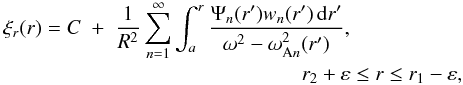 (53)where C and a are constants, and r2 + ε < a < r1 − ε. Using these results we obtain
 ![Mathematical equation: \begin{eqnarray} [\xi_r]_1 = \xi_r(R+\ell/2) &-& C - \frac1{R^2}{\cal P}\int_a^{R+\ell/2} \frac{\Psi_1(r)w_1(r)\,{\rm d}r}{\omega^2 - \omega_{\rm A1}^2(r)} \nonumber\\ &-& \frac1{R^2}\sum_{n=2}^\infty\int_a^{R+\ell/2} \frac{\Psi_n(r)w_n(r)\,{\rm d}r}{\omega^2 - \omega_{{\rm A}n}^2(r)}, \label{eq:4.30} \end{eqnarray}](/articles/aa/full_html/2011/10/aa17416-11/aa17416-11-eq204.png) (54)where
(54)where  indicates the principal Cauchy part of the integral. Comparing this expression with Eq. (47) yields
 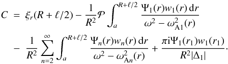 (55)Substituting this expression in Eq. (53) we obtain the expression for ξr valid for r2 < r ≤ R + ℓ/2,
 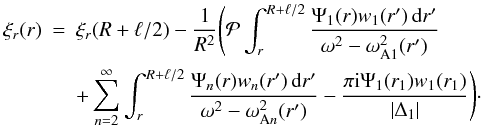 (56)Continuing this procedure we eventually arrive at the expression for ξr valid for R − ℓ/2 ≤ r ≤ R + ℓ/2,
 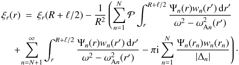 (57)It follows from this expression that
  (58)
(58)
4.3. Governing equation for amplitude
Using Eqs. (42) and (58) we are now in the position to express δS and δP in terms of S0. It follows from Eqs. (18), (25) and (29) that ![Mathematical equation: \begin{equation} \epsilon^2 Q_{\rm i} = \frac{\omega^2}2R(\rho_{\rm i} - \rho_{\rm e})S_0 \exp({\rm i}\nu^{-1}\Theta)[1 + {\cal O}(\nu)]. \label{eq:4.34} \end{equation}](/articles/aa/full_html/2011/10/aa17416-11/aa17416-11-eq212.png) (59)Substituting this result in Eq. (42) we obtain
(59)Substituting this result in Eq. (42) we obtain ![Mathematical equation: \begin{equation} \delta P = \frac{\ell\omega^2}2(\rho_{\rm i} - \rho_{\rm e})S_0 \exp({\rm i}\nu^{-1}\Theta)[1 + {\cal O}(\nu)]. \label{eq:4.35} \end{equation}](/articles/aa/full_html/2011/10/aa17416-11/aa17416-11-eq213.png) (60)The variation of P across the transitional layer is of the order of ν. Since we calculate δS in the leading order approximation with respect to ν, we can take P = ϵ2Qi when calculating δS. Hence we can substitute
(60)The variation of P across the transitional layer is of the order of ν. Since we calculate δS in the leading order approximation with respect to ν, we can take P = ϵ2Qi when calculating δS. Hence we can substitute  (61)
in Eq. (58). Then, introducing function
(61)
in Eq. (58). Then, introducing function
 and its Fourier coefficients Φn we obtain that δS is given by
  (62)Substituting Eqs. (60) and (62) in Eq. (37) we obtain with the aid of Eq. (38)
 ![Mathematical equation: \begin{eqnarray} \frac{\rm d}{{\rm d}t}&&\hspace*{-5mm}\left(\omega\int_{-L/2}^{L/2} \frac{S_0^2}{C_{\rm k}^2}\,{\rm d}z\right) = \frac{{\rm i}\mu_0\omega^2}{2RB^2} \int_{-L/2}^{L/2}S_0 \nonumber\\ &\times& \left(\sum_{n=1}^N{\cal P}\int_{R-\ell/2}^{R+\ell/2} \frac{[\rho_{\rm t}(r)\omega_{{\rm A}n}^2(r) - \rho_{\rm e}\omega^2]\Phi_n(r)w_n(r)\,{\rm d}r} {\omega^2 - \omega_{{\rm A}n}^2(r)}\right.\nonumber\\ &+& \left.\sum_{n=N+1}^\infty\int_{R-\ell/2}^{R+\ell/2} \frac{[\rho_{\rm t}(r)(r) - \rho_{\rm e}\omega^2]\Phi_n(r)w_n(r)\,{\rm d}r} {\omega^2 - \omega_{{\rm A}n}^2(r)}\right){\rm d}z \nonumber\\ &-& \frac{\pi\mu_0\omega^4}{2RB^2} \sum_{n=1}^N\int_{-L/2}^{L/2} \frac{[\rho_{\rm t}(r_n) - \rho_{\rm e}]S_0\Phi_n(r_n)w_n(r_n)}{|\Delta_n|}{\rm d}z. \label{eq:4.38} \end{eqnarray}](/articles/aa/full_html/2011/10/aa17416-11/aa17416-11-eq219.png) (63)Let W0(t,z) be solution to Eq. (31) satisfying the boundary conditions (32) that corresponds to the fundamental mode. We take W0 to be real. Since the eigenfunction describing the fundamental mode has no nodes, we can take W0 > 0. Finally, since an eigenfunction multiplied by an arbitrary function of t is once again an eigenfunction, we can take max(W0) = 1, where the maximum is calculated with respect to z at a fixed t. The general solution corresponding to the fundamental mode is
(63)Let W0(t,z) be solution to Eq. (31) satisfying the boundary conditions (32) that corresponds to the fundamental mode. We take W0 to be real. Since the eigenfunction describing the fundamental mode has no nodes, we can take W0 > 0. Finally, since an eigenfunction multiplied by an arbitrary function of t is once again an eigenfunction, we can take max(W0) = 1, where the maximum is calculated with respect to z at a fixed t. The general solution corresponding to the fundamental mode is ![Mathematical equation: \begin{equation} S_0(t,z) = A(t)W_0(t,z)\exp[{\rm i}F(t,z)], \label{eq:4.39} \end{equation}](/articles/aa/full_html/2011/10/aa17416-11/aa17416-11-eq224.png) (64)where A(t) > 0 and F(t) are real functions. Since max|S0| = A, the function A(t) is the oscillation amplitude at the instant t. It follows from Eq. (41) and the definition of the Alfvén speed that
(64)where A(t) > 0 and F(t) are real functions. Since max|S0| = A, the function A(t) is the oscillation amplitude at the instant t. It follows from Eq. (41) and the definition of the Alfvén speed that 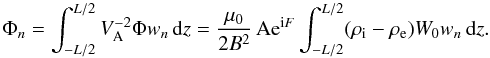 (65)Substituting Eqs. (64) and (65) in Eq. (63) we obtain
 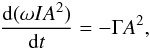 (66)
(66) (67)where
 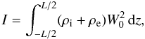 (68)
(68)![Mathematical equation: \begin{eqnarray} \Gamma &=& -\frac{\pi\mu_0\omega^4}{2RB^2}\sum_{n=1}^N \int_{-L/2}^{L/2}(\rho_{\rm i}-\rho_{\rm e})W_0 w_n(r_n)\,{\rm d}z \nonumber\\ &&\times\int_{-L/2}^{L/2}\frac{[\rho_{\rm t}(r_n)-\rho_{\rm e}]W_0 w_n(r_n)}{|\Delta_n|}{\rm d}z, \label{eq:4.44} \end{eqnarray}](/articles/aa/full_html/2011/10/aa17416-11/aa17416-11-eq233.png) (69)
(69)![Mathematical equation: \begin{eqnarray} \Upsilon = \frac{\mu_0\omega}{4RB^2 I}\hspace*{-5mm}&& \left\{\sum_{n=1}^N {\cal P}\int_{R-\ell/2}^{R+\ell/2} \left(\int_{-L/2}^{L/2}(\rho_{\rm i}-\rho_{\rm e})W_0 w_n(r_n)\,{\rm d}z \right.\right. \nonumber\\ &\times& \left.\int_{-L/2}^{L/2} \frac{[\rho_{\rm t}(r)\omega_{{\rm A}n}^2(r) - \rho_{\rm e}\omega^2] W_0 w_n(r)}{\omega^2 - \omega_{{\rm A}n}^2(r)}{\rm d}z\right){\rm d}r \nonumber\\ &+& \sum_{n=N+1}^\infty \int_{R-\ell/2}^{R+\ell/2} \left(\int_{-L/2}^{L/2}(\rho_{\rm i}-\rho_{\rm e})W_0 w_n(r_n)\,{\rm d}z \right. \nonumber\\ &\times& \left.\left(\int_{-L/2}^{L/2} \frac{[\rho_{\rm t}(r)\omega_{{\rm A}n}^2(r) - \rho_{\rm e}\omega^2] W_0 w_n(r)}{\omega^2 - \omega_{{\rm A}n}^2(r)}{\rm d}z\right){\rm d}r\right\}. \label{eq:4.45} \end{eqnarray}](/articles/aa/full_html/2011/10/aa17416-11/aa17416-11-eq234.png) (70)The multiplier exp [iF(t)] describes only a small phase shift of the oscillations. Since we are mainly interested in the amplitude dependence on time, we will use only Eq. (66) in what follows.
(70)The multiplier exp [iF(t)] describes only a small phase shift of the oscillations. Since we are mainly interested in the amplitude dependence on time, we will use only Eq. (66) in what follows.
5. Kink oscillations of coronal loops with barometric density distribution
5.1. Kink oscillations of static coronal loops
To verify the accuracy of Eq. (66) we apply it to studying the damping of kink oscillations of static coronal loops and compare the results with those obtained in previous studies. For static loops Eq. (66) reduces to 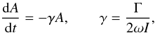 (71)so the oscillation amplitude decreases exponentially with the decrement γ. Let us introduce ζ = ρi(L/2)/ρe(L/2). Now we make the same assumptions as in Paper II. We assume that ρi(z)/ρe(z) = ζ and ρt(r,z) = f(r)ρi(z), where f(r) is a monotonically decreasing function, f(R − ℓ/2) = 1, f(R + ℓ/2) = 1/ζ. In particular, we obtain such an equilibrium if we assume that the plasma is isothermal with equal temperatures inside and outside the loop, and use the barometric formula for the density. It is shown in Paper II that, when ρt(r,z) = f(r)ρi(z), we can take wn independent of r, while the eigenvalue dependence on r is given by
  (72)In what follows we assume that there is only one resonant position, r = r1, so N = 1 in Eqs. (69) and (70). Equation (31) become
  (73)Equation (38) for the fundamental harmonic at r = r1 takes the form
  (74)It is obvious that the resonant condition is satisfied only when the coefficient functions at the second derivative at these two equations coincide. This gives
  (75)Substituting Eq. (72) in Eq. (45) and using Eqs. (75) we obtain
 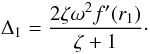 (76)Since W0 and w1(r1) are the eigenfunctions of the same eigenvalue problem corresponding to the same eigenvalue, we have W0(z) = w1(r1,z). Using this result and Eq. (76) we transform the expression for γ to
 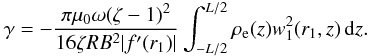 (77)Using Eq. (40) we obtain
 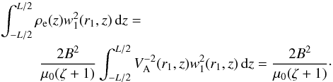 (78)Substituting this result in Eq. (77) we arrive at
 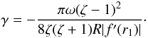 (79)This expression coincides with the expression for γ given by Eq. (82) in Paper II if we substitute in this equation Δ1 given by Eq. (76). When f(r) is a linear function given by
  (80)the expression for γ reduces to
  (81)which coincides with the expression used by Goossens et al. (2002; see also the review papers by Goossens et al. 2006; and Ruderman & Erdélyi 2009). For the sinusoidal density profile determined by
  (82)we obtain from Eq. (75) that r1 = R. Then Eq. (79) reduces to
  (83)obtained by Ruderman & Roberts (2002). Note that both Goossens et al. (2002) and Ruderman & Roberts (2002) considered magnetic tubes with the density that depends on r only, while in this paper we consider the density varying along the loop. Dymova & Ruderman (2006) showed that, under the assumption that ρe/ρi = const. and ρt/ρi is independent of z, the ratio γ/ω is the same for any function ρi(z). In view of this result the coincidence of the expressions for γ/ω given by Eqs. (81) and (83) with those in Goossens et al. (2002) and Ruderman & Roberts (2002), respectively, is not surprising.
5.2. Kink oscillations of cooling coronal loops
In this subsection we once again assume that there is only one resonant position r = r1. Similar to Paper I we also assume that the plasma temperature outside the loop, T0, does not change with time, while it decreases inside the loop due to the radiative cooling. Following Aschwanden & Terradas (2008) and Morton & Erdélyi (2010) we approximate the temperature evolution inside the loop by an exponentially decaying function, 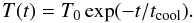 (84)In accordance with the equation of mass conservation the temperature variation with time causes the plasma flow, so the plasma inside the tube is not in the hydrostatic equilibrium, and the density distribution is not described by the barometric formula. However it was shown in Paper I that, for typical flow velocities observed in coronal loops, the flow effect on the density distribution is weak, and the barometric formula for the density is a good approximation. Hence, we use the barometric formula for the density both inside and outside the loop. Then, assuming that the loop has a half-circle shape, we obtain
 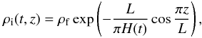 (85)
(85) (86)where ρf = const. is the density at the foot points inside the loop,
 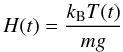 (87)is the atmospheric scale height, H0 = H(0), kB is the Boltzmann constant, m is the mean mass per particle (equal to one half of the proton mass for the proton-electron plasma), and g is the gravitational acceleration. We further assume that the density profile in the transitional layer is linear, so
 ![Mathematical equation: \begin{equation} \rho_{\rm t}(t,r,z) = \frac12[\rho_{\rm i}(t,z) + \rho_{\rm e}(z)] + [\rho_{\rm i}(t,z) - \rho_{\rm e}(z)]\frac{R-r}\ell\cdot \label{eq:5.18} \end{equation}](/articles/aa/full_html/2011/10/aa17416-11/aa17416-11-eq275.png) (88)We see that ρt = (ρi + ρe)/2 when r = R, so VA(R,z) = Ck(z). Then it follows that Eq. (38) coincides with Eq. (31) when r = R and, therefore,
(88)We see that ρt = (ρi + ρe)/2 when r = R, so VA(R,z) = Ck(z). Then it follows that Eq. (38) coincides with Eq. (31) when r = R and, therefore,  . Hence we conclude that r1 = R and, as in the previous subsection, W0(z)/w1(R,z) is a constant. Recall that we consider only the fundamental mode. Since the equilibrium is symmetric with respect to the apex point, it follows that W0(z) is an even function. Then it takes its maximum value at z = 0, and the condition max(W0) = 1 reduces to W0(0) = 1. Using this condition we obtain
 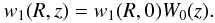 (89)It follows from Eq. (40) and the relation VA(R) = Ck that
 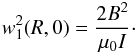 (90)Differentiating Eq. (38) with respect to r and then taking r = R we obtain, with the aid of Eq. (89),
 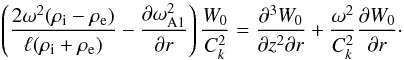 (91)Multiplying this equation by W0, integrating with respect to z, and using the integration by parts and the boundary conditions W0( ± L/2) = 0 yields
 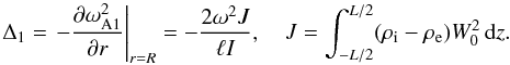 (92)Using Eqs. (88)–(90) and (92) we obtain
 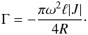 (93)Let us introduce the dimensionless variables and parameters
 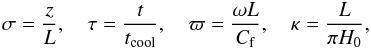 (94)where
 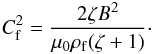 (95)Since we solve a linear problem, we can fix A at the initial moment of time arbitrarily. We take A(0) = 1, so that A(t) is just the ratio of the current and initial oscillation amplitude. We rewrite Eq. (31) with W0 substituted for S0 in the dimensionless form as
 ![Mathematical equation: \begin{equation} \frac{\partial^2 W_0}{\partial\sigma^2} + \frac{\varpi^2 W_0}{\zeta + 1} \left[\zeta\exp(-\kappa {\rm e}^\tau\cos(\pi\sigma)) + \exp(-\kappa\cos(\pi\sigma))\right]= 0. \label{eq:5.26} \end{equation}](/articles/aa/full_html/2011/10/aa17416-11/aa17416-11-eq295.png) (96)Since we only consider the fundamental mode and the loop is symmetric with respect to the apex point, we can use the boundary conditions
(96)Since we only consider the fundamental mode and the loop is symmetric with respect to the apex point, we can use the boundary conditions 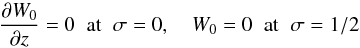 (97)instead of the boundary conditions (32). Recall that W0(0) = 1. The dimensionless form of Eq. (66) with Γ given by Eq. (93) is
 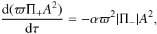 (98)where
 ![Mathematical equation: \begin{equation} \Pi_\pm = \int_0^{1/2}W_0^2\left[\zeta\exp(-\kappa {\rm e}^\tau\cos(\pi\sigma)) \pm \exp(-\kappa\cos(\pi\sigma))\right]\,{\rm d}\sigma, \label{eq:5.29} \end{equation}](/articles/aa/full_html/2011/10/aa17416-11/aa17416-11-eq299.png) (99)and the parameter
(99)and the parameter 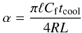 (100)determines the relative strength of resonant damping and amplification due to cooling. When deriving the expression for Π ± we have taken into account that W0, ρi(z) and ρe(z) are even functions.
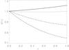 |
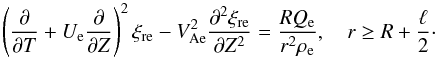
Fig. 1 The dependence of the relative amplitude A on the dimensionless time τ for ζ = 3 and κ = 0.5. The solid, dotted, dashed and dashed-dotted curves correspond to α = 0, 0.13, 0.5, and 1.0 respectively. |
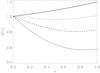 |
Fig. 2 The same as Fig. 1, but for ζ = 3 and κ = 1. The solid, dotted, dashed and dashed-dotted curves correspond to α = 0, 0.22, 0.5, and 1.0 respectively. |
We see that the dependence of the oscillation amplitude A on time is determined by the three non-dimensional parameters, α, ζ and κ. The function A(t) is calculated numerically for various values of α, ζ and κ. The results of these calculations are presented in Figs. 1–6.
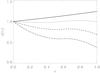 |
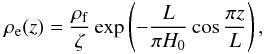
Fig. 3 The same as Fig. 1, but for ζ = 3 and κ = 2. The solid, dotted, dashed and dashed-dotted curves correspond to α = 0, 0.19, 0.5, and 1.0 respectively. |
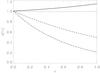 |
Fig. 4 The same as Fig. 1, but for ζ = 10 and κ = 0.5. The solid, dotted, dashed and dashed-dotted curves correspond to α = 0, 0.08, 0.5, and 1.0 respectively. |
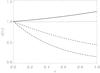 |
Fig. 5 The same as Fig. 1, but for ζ = 10 and κ = 1. The solid, dotted, dashed and dashed-dotted curves correspond to α = 0, 0.1, 0.5, and 1.0 respectively. |
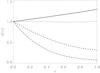 |
Fig. 6 The same as Fig. 1, but for ζ = 10 and κ = 2. The solid, dotted, dashed and dashed-dotted curves correspond to α = 0, 0.08, 0.5, and 1.0 respectively. |
Let us introduce the critical value of α, αc, defined by the condition that, for this value of α, A(1) = A(0), i.e. the oscillation amplitude at t = tcool is equal to the initial amplitude. We also introduce the critical value of the transitional layer thickness, ℓc, defined by 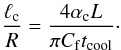 (101)When ℓ = ℓc the amplification due to cooling is in balance with damping due to resonant absorption. Using Figs. 1–6 we obtain the following values of αc for various values of ζ and κ:
Values of αc for various values of ζ and κ.
This table shows that αc decreases when ζ increases. The dependence of αc on κ is non-monotonic and, for ζ = 10, very weak.
It is worth noting the non-monotonic behaviour of the dotted, dashed and dashed-dotted curves in Figs. 2 and 3. It is related to the fact that, for ζ = 3 and κ = 1 and 2, the function Π − (t) changes the sign: while Π − (0) > 0, Π − (t) < 0 for sufficiently large t, so there is such t0 that Π − (t0) = 0. The right-hand side of Eq. (98) is very small for t close to t0. For these values of t the resonant damping is very weak and the amplification due to cooling dominates.
We also note that the condition ρi(z) > ρe(z) for all z ∈ [−L/2,L/2] is violated for ζ = 3 and κ = 1 and 2, and also for ζ = 10 and κ = 2. However in all these cases there is still only one resonant position. It seems that the kink mode becomes leaky for sufficiently large values of t when ζ = 3 and κ = 2 and, may be, also when ζ = 3 and κ = 1. If this is the case then there is an additional damping due to leakage. However, in the thin tube approximation, this damping is very small and can be safely neglected. Having this in mind we did not study this problem further.
We are now in the position to give a more accurate estimate of the transitional layer thickness in the event reported by Aschwanden & Schrijver (2011). In this oscillation event the initial oscillation period was Pinit = 395 s. It was estimated in Paper I that κ ≈ 1 and tcool ≈ 2050 s. and, following this paper, we take ζ = 10. Since in the initial moment of time ρi(z)/ρe(z) = const., it follows from Eq. (96) that ϖ(0) is independent of ζ. Then we can use Fig. 4 in Paper I to obtain ϖ(0) ≈ 4.8 for κ = 1. Now, using the relation ϖ(0) = 2πL/PinitCf, we find L/Cf ≈ 300 s. It follows from Table 1 that αc ≈ 0.1 for ζ = 10 and κ = 1. Substituting these values in Eq. (101) we obtain ℓc/R ≈ 0.02, which is about twice smaller than the crude estimate obtained in Paper I. Hence the conclusion made both by Aschwanden & Schrijver (2011) and in Paper I that the observed oscillation could stay undamped only if the transitional inhomogeneous layer is extremely thin remains valid.
The ability of amplification due to cooling to balance the resonant damping strongly depends on the characteristics of the oscillating loop and on the cooling time. As an example, consider a loop with ζ = 3 and κ = 1. In this case αc ≈ 0.22 and, once again in accordance with Fig. 4 in Paper I, ϖ(0) ≈ 4.8. Substituting these numbers in Eq. (101) we obtain 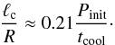 (102)If we now take tcool = Pinit, then we obtain ℓc/R ≈ 0.21, which is in the range of values of ℓ/R typical for non-cooling loops (see, e.g. Goossens et al. 2002). Recall that the analysis in this section has been carried out under the assumption that tcool ≫ Pinit, so it is questionable if Eq. (102) remains valid for tcool = Pinit. For such a short cooling time the problem should be solved numerically without using the WKB method.
One concluding remark concerns the oscillation period. Since cooling causes the evacuation of plasma from the loop, the average plasma density in the loop decreases and, consequently, the frequency of kink oscillations increases. Theoretically this problem has been comprehensively studied by Morton & Erdélyi (2009) and in Paper I for the loop model with the sharp boundary. In particular, in Paper I the time dependence of the oscillation frequency for the model of cooling loop considered in this subsection was calculated. Since the presence of the transitional layer at the tube boundary does not affect the oscillation frequency in the TB approximation, there is no need to address the problem of frequency increase in this paper.
As for the comparison with the observations, we first of all note that the observational evidence of frequency decrease was found in the wavelet analysis by De Moortel et al. (2004). They reported a 35% decrease in the oscillation period in the event reported by Nakariakov et al. (1999). The problem of the period decrease has been also addressed by Morton & Erdélyi (2010) who found that the analytical profile with increasing frequency fits better the observational data than the profile with the constant frequency. On the other hand, the period decrease has not been found in any other papers analyzing observations of coronal loop kink oscillations, including the paper by Aschwanden & Schrijver (2011), which is not surprising at all. The point is that, in all these papers, the best fit to the data has been carried out using the function e − γtsin(ωt − θ). Hence, it has been assumed from the very beginning that the oscillation frequency is constant. To determine the frequency variation we need to use the function given by Eq. (25) with Θ and S calculated numerically using the procedure presented in this paper. The best fit must be carried out with respect to the initial phase of the oscillation, tcool and ν = ℓ/R. In this way we can verify and, possibly, correct the value of cooling time found from the direct observation of the loop temperature. We can also obtain the estimate of the transitional layer thickness. At present this analysis of observations of cooling loop kink oscillations is in progress.
6. Summary and conclusions
In this paper we have studied the resonant damping of kink oscillations of cooling coronal loops. We modelled the loop by a straight magnetic cylinder that consists of the core region and transitional layer. The magnetic field is straight and has constant magnitude everywhere. In the core region and outside the loop the plasma density varies only along the loop, while in the transitional layer it also varies in the radial direction from its value inside the core region to its value outside the loop. In addition, the density varies with time. The time-dependence of the density causes the plasma flow along the loop. The plasma motion is described by the linearized MHD equations in the cold plasma approximation. Using the quasi-Lagrangian description and the thin tube approximation we derived the equation governing the displacement of the loop axis. This equation is not closed because, in addition to the loop axis displacement, it contains the jumps of the plasma displacement and magnetic pressure perturbation across the inhomogeneous layer. When there is no inhomogeneous layer and the loop has a sharp boundary, this equation reduces to the corresponding equation previously derived in Paper I.
The effects of cooling and resonant damping have been studied under the assumption that both the characteristic cooling time and damping time are much larger than the characteristic oscillation period. The second assumption implies that we use the thin boundary layer approximation. The two assumptions enabled us to use the WKB method. With the use of this method and the connection formulae we calculated the jumps of the plasma displacement and magnetic pressure perturbation across the inhomogeneous layer and obtained the closed equation for the loop axis displacement under the assumption that the radial dependence of the density is linear. Then we derived the equation describing the time-variation of the so-called adiabatic invariant for the loop kink oscillations first introduced in Paper I. When the loop has a sharp boundary the adiabatic invariant is conserved. The equation for the adiabatic invariant determines the time-dependence of the amplitude of the loop oscillation.
We further assumed that cooling occurs only inside the loop, while the temperature of the external plasma does not change. We also assumed that the loop has a half-circle shape, the initial plasma temperature is the same inside and outside the loop, and it is constant, and the density dependence on the height is described by the barometric formula. Finally, we assumed that the temperature inside the loop decreases exponentially. Under these assumptions the equation for the oscillation amplitude written in the dimensionless form contains three dimensionless parameters: the ratio of densities inside and outside the loop at the initial moment of time ζ > 1, the ratio of the loop height to the initial atmospheric scale height κ, and the parameter α
characterizing the efficiency of the resonant damping. The latter parameter is proportional to the ratio of the transitional layer thickness ℓ to the radius of the loop cross-section R.
The equation for the oscillation amplitude was solved numerically for various values of ζ, κ and α. The most interesting problem was to study when the amplification of the oscillation amplitude due to cooling can balance the resonant damping to produce undamped oscillations. We consider the oscillation as undamped if its amplitude at the time equal to the characteristic cooling time tcool is the same as at the initial moment of time. We denote the value of α corresponding to undamped oscillations as αc, and the corresponding value of ℓ as ℓc. The quantity αc is given in Table 1 for various values of ζ and κ. This quantity decreases when ζ increases, while its dependence of κ is non-monotonic. When ζ = 10, αc is almost independent of κ. On the basis of the numerical results we can make the conclusion that, in general, the amplification due to cooling is not very efficient. It can balance the resonant damping and produce undamped oscillations of loops with typical values of ℓ/R (ℓ/R ≳ 0.2) only when ζ is sufficiently small (ζ ≲ 3) and the cooling occurs very quickly with tcool of the order of the oscillation period.
References
- Aschwanden, M. J., & Schrijver, C. J. 2011, ApJ, 736, 102 [NASA ADS] [CrossRef] [Google Scholar]
- Aschwanden, M. J., & Terradas, J. 2008, ApJ, 686, L127 [NASA ADS] [CrossRef] [Google Scholar]
- Aschwanden, M. J., Fletcher, L., Schrijver, C. J., & Alexander, D. 1999, ApJ, 520, 880 [NASA ADS] [CrossRef] [Google Scholar]
- Aschwanden, M. J., de Pontieu, B., Schrijver, C. J., & Title, A. M. 2002, Sol. Phys., 206, 99 [NASA ADS] [CrossRef] [Google Scholar]
- Bender, C. M., & Orszag, S. A. 1978, Advanced Mathematical Methods for Scientists and Engineers (New York: McGraw-Hill) [Google Scholar]
- Coddington, E. A., & Levinson, N. 1978, Theory of Ordinary Differential Equations (New York: McGraw-Hill) [Google Scholar]
- De Moortel, I., & Brady, C. S. 2007, ApJ, 664, 1210 [NASA ADS] [CrossRef] [Google Scholar]
- De Moortel, I., Munday, S. A., & Hood, A. W. 2004, Sol. Phys., 222, 203 [NASA ADS] [CrossRef] [Google Scholar]
- Dymova, M. V., & Ruderman, M. S. 2005, Sol. Phys., 229, 79 [NASA ADS] [CrossRef] [Google Scholar]
- Dymova, M. V., & Ruderman, M. S. 2006, A&A, 457, 1059 [NASA ADS] [CrossRef] [EDP Sciences] [Google Scholar]
- Goossens, M., Andries, J., & Aschwanden, M. J. 2002, A&A, 394, L39 [NASA ADS] [CrossRef] [EDP Sciences] [Google Scholar]
- Goossens, M., Andries, J., & Arregui, I. 2006, Phil. Trans. R. Soc. A, 364, 433 [NASA ADS] [CrossRef] [Google Scholar]
- Morton, R. J., & Erdélyi, R. 2009, ApJ, 707, 750 [NASA ADS] [CrossRef] [Google Scholar]
- Morton, R. J., & Erdélyi, R. 2010, A&A, 519, A43 [NASA ADS] [CrossRef] [EDP Sciences] [Google Scholar]
- Morton, R., Hood, A., & Erdélyi, R. 2009, A&A, 512, A23 [Google Scholar]
- Naimark, M. A. 1967, Linear Differential Equations, Part I [Google Scholar]
- Nakariakov, V. M., Ofman, L., Deluca, E. E., Roberts, B., & Davila, J. M. 1999, Science, 285, 862 [NASA ADS] [CrossRef] [PubMed] [Google Scholar]
- Ruderman, M. S. 2010, Sol. Phys., 267, 377 [NASA ADS] [CrossRef] [Google Scholar]
- Ruderman, M. S. 2011a, Sol. Phys., 271, 55 [NASA ADS] [CrossRef] [Google Scholar]
- Ruderman, M. S. 2011b, Sol. Phys., 271, 41 [NASA ADS] [CrossRef] [Google Scholar]
- Ruderman, M. S., & Erdélyi, R. 2009, Space Sci. Rev., 149, 199 [NASA ADS] [CrossRef] [Google Scholar]
- Ruderman, M. S., & Roberts, B. 2002, ApJ, 577, 475 [NASA ADS] [CrossRef] [Google Scholar]
- Ruderman, M. S., & Scott, A. 2011, A&A, 529, A33 [NASA ADS] [CrossRef] [EDP Sciences] [Google Scholar]
- Titchmarsh, E. C. 1946, Eigenfunction Expansions Associated with 2nd-order Differential Equations [Google Scholar]
All Tables
All Figures
|
Fig. 1 The dependence of the relative amplitude A on the dimensionless time τ for ζ = 3 and κ = 0.5. The solid, dotted, dashed and dashed-dotted curves correspond to α = 0, 0.13, 0.5, and 1.0 respectively. |
| In the text | |
|
Fig. 2 The same as Fig. 1, but for ζ = 3 and κ = 1. The solid, dotted, dashed and dashed-dotted curves correspond to α = 0, 0.22, 0.5, and 1.0 respectively. |
| In the text | |
|
Fig. 3 The same as Fig. 1, but for ζ = 3 and κ = 2. The solid, dotted, dashed and dashed-dotted curves correspond to α = 0, 0.19, 0.5, and 1.0 respectively. |
| In the text | |
|
Fig. 4 The same as Fig. 1, but for ζ = 10 and κ = 0.5. The solid, dotted, dashed and dashed-dotted curves correspond to α = 0, 0.08, 0.5, and 1.0 respectively. |
| In the text | |
|
Fig. 5 The same as Fig. 1, but for ζ = 10 and κ = 1. The solid, dotted, dashed and dashed-dotted curves correspond to α = 0, 0.1, 0.5, and 1.0 respectively. |
| In the text | |
|
Fig. 6 The same as Fig. 1, but for ζ = 10 and κ = 2. The solid, dotted, dashed and dashed-dotted curves correspond to α = 0, 0.08, 0.5, and 1.0 respectively. |
| In the text | |
Current usage metrics show cumulative count of Article Views (full-text article views including HTML views, PDF and ePub downloads, according to the available data) and Abstracts Views on Vision4Press platform.
Data correspond to usage on the plateform after 2015. The current usage metrics is available 48-96 hours after online publication and is updated daily on week days.
Initial download of the metrics may take a while.